First Stellar Abundances in the Dwarf Irregular Galaxy Sextans A

Abstract

We present the abundance analyses of three isolated A-type supergiant stars in the dwarf irregular galaxy Sextans A (catalog ) (= DDO 75) from high-resolution spectra obtained with Ultraviolet-Visual Echelle Spectrograph (UVES) on the Kueyen telescope (UT2) of the ESO Very Large Telescope (VLT). Detailed model atmosphere analyses have been used to determine the stellar atmospheric parameters and the elemental abundances of the stars. The mean iron group abundance was determined from these three stars to be $\left<[({\rm Fe\,II,Cr\,II})/{\rm H}]\right>=-0.99\pm 0.04\pm{\it 0.06}$. This is the first determination of the present-day iron group abundances in Sextans A. These three stars now represent the most metal-poor massive stars for which detailed abundance analyses have been carried out.

The mean stellar $\alpha$ element abundance was determined from the $\alpha$ element magnesium as $\left<[\alpha({\rm Mg\,I})/{\rm H}]\right>=-1.09\pm 0.02\pm{\it 0.19}$. This is in excellent agreement with the nebular $\alpha$ element abundances as determined from oxygen in the H II regions. These results are consistent from star-to-star with no significant spatial variations over a length of  $0.8$ kpc in Sextans A. This supports the nebular abundance studies of dwarf irregular galaxies, where homogeneous oxygen abundances are found throughout, and argues against in situ (“on the spot”) enrichment.

The $\alpha/{\rm Fe}$ abundance ratio is $\left<[\alpha({\rm Mg\,I})/{\rm Fe\,II,Cr\,II}]\right>=-0.11\pm 0.02\pm{\it 0.10}$, which is slightly lower but consistent with the solar ratio. This is consistent with the results from A-supergiant analyses in other Local Group dwarf irregular galaxies, NGC 6822 and WLM. The results of near solar [$\alpha$/Fe] ratios in dwarf galaxies is in stark contrast with the high [$\alpha$/Fe] results from metal-poor stars in the Galaxy (which plateau at values near +0.4 dex), and is most clearly seen from these three stars in Sextans A because of their lower metallicities. The low [$\alpha$/Fe] ratios are consistent with the slow chemical evolution expected for dwarf galaxies from analyses of their stellar populations.

1 Introduction

Dwarf irregular galaxies (dIrrs) are low mass, but gas rich galaxies and are found rather isolated and spread throughout the Local Group. All dIrrs display low elemental abundances indicating that only little chemical evolution has taken place over the past 15 Gyr despite ongoing star formation. The lack of strong starburst cycles in these isolated objects may be because of little or no merger interaction. Therefore, in the context the cold dark matter scenarios of hierarchical galaxy formation by merger of smaller structures (Steinmetz & Navarro, 1999), dwarf galaxies and in particular the isolated dwarf irregular galaxies could be the purest remnants of the proto-galactic fragments from the early Universe. Hence, the dIrrs are also one of the possible sources for the damped Ly$\alpha$ absorption (DLA) systems as observed in quasar spectra over a large range of redshifts; see e.g. Prochaska et al. (2003) for a recent compilation of DLA metallicities over $0.5<z<5$. The dIrrs being possible remnants of the early Universe might allow us to study early galaxy evolution in great detail in the nearby universe, even in the Local Group. In particular the early chemical evolution of galaxies is of interest here to shed light on the formation of the first generations of stars. The most powerful way to study the chemical evolution of a galaxy is via the elemental abundances and abundance ratios of their stellar and gas content which contain a record of the star formation histories (SFH) of the galaxy over the last 15 Gyr.

The analysis of bright nebular emission lines of H II regions has been the most frequent approach to modeling chemical evolution of more distant galaxies to date (Matteucci & Tosi, 1985). So far, only a very limited number of elements can be examined and quantified when using this approach. The chemical evolution of a galaxy depends on the contributions of all its constituents, e.g., SNe type Ia and II, high mass stars, thermal pulsing in low and intermediate mass AGB stars. Thus, more elements than just those observed in nebulae need to be measured, since each have different formation sites which sample different constituents. The $\alpha$ elements like oxygen are created primarily in short-lived massive stars, while the iron-group elements are produced in SNe of both high and low mass stars. Therefore, it is expected that substantially different SFHs of individual galaxies shall be represented in different present-day $\alpha/{\rm Fe}$ ratios as discussed e.g. in Gilmore & Wyse (1991). In reverse, the accurate measurement of the absolute stellar abundances and abundance ratios allows to put constraints on the SFH of the respective galaxy. In addition to the study of the average metallicities of a galaxy as discussed above, also the spatial distribution of abundances and abundance patterns within a galaxy contains important information about the redistribution processes of the newly produced elements and their subsequent mixing with the ISM. If the abundances of a number of stars distributed over the galaxy can be analyzed, possible chemical inhomogeneities e.g. in form of large spreads in the abundances or abundance gradients can be studied and provide additional constraints of the chemo-dynamical evolution of the galaxy.

Unfortunately, most dIrr systems are too distant for the detailed study and abundance analyses of e.g. their red giant branch (RGB) stars, which are of great importance due to their large spread in age. Hence, to date few details on the chemical evolution of the dIrr galaxies have been available. In the case of the dIrr Sextans A studied in this work the tip of the RGB is found at visual magnitudes of $V\approx 23$ (Dohm-Palmer et al., 2002) — far beyond the capabilities of even the most efficient high-resolution spectrographs on today’s 8 to 10-meter class telescopes. However, with the same class of latest telescopes and instrumentation, the visually brightest stars of the dIrr galaxies, i.e., the blue supergiants ($17.5\lesssim V\lesssim 20$ in Sextans A) become now accessible to detailed spectroscopy, which allow us to determine the present-day abundances of $\alpha$ and iron group elements. The abundances of the $\alpha$ elements derived from the rich spectra of hot massive stars can be directly compared and tied to the nebular $\alpha$ element abundances because both nebulae and massive stars have comparable ages and the same formation sites. The first abundance studies based on high-resolution spectra of A-type supergiant stars were carried out for the nearby Local Group dIrrs NGC 6822 and WLM (Venn et al., 2001, 2003a). $\alpha$ element and iron group abundances could be derived for two stars in both dIrr galaxies. For NGC 6822 and WLM the [$\alpha/{\rm Fe}$] ratios are in good agreement with the solar ratio. This result is somewhat surprising since both galaxies have ongoing star formation and different star formation histories as determined from their stellar populations (e.g., Gallart et al. (1996), Mateo (1998), Dolphin et al. (2003a)).

The isolated dwarf irregular galaxy Sextans A (= DDO 75) with its distance of about $1.3$ Mpc (Dolphin et al., 2003a) is located at a similar distance as Sextans B, NGC 3109, and the Antlia dwarf galaxies which form a small group of galaxies at the edge of the Local Group — possibly not even bound to the Local Group which would make Sextans A a member of the nearest (sub)cluster of galaxies (van den Berg, 1999). The present-day chemical composition was studied from the emission-line spectroscopy of bright compact H II regions (Hodge et al., 1994). The analysis by Skillman et al. (1989) determines an oxygen abundance of $12+\log(\rm{O/H})=7.49$ which corresponds to $[\rm{O/H}]=-1.17$ if a solar oxygen abundance of $12+\log(\rm{O/H})_{\odot}=8.66$ is adopted (Asplund, 2003). In a revised analyses of the same data by Pilyugin (2001), a higher value of $12+\log(\rm{O/H})=7.71$ is found, corresponding to $[\rm{O/H}]=-0.95$. The star formation history of Sextans A was first studied in detail by Dohm-Palmer et al. (1997), and more recently by Dohm-Palmer et al. (2002) and Dolphin et al. (2003b) using HST VI color – magnitude diagrams (CMD). A high rate of star formation has occured in the past $~{}2.5$ Gyr, with very little star formation between $2.5$ and $10$ Gyrs. A mean metallicity of $[\rm{M/H}]\approx-1.45\pm 0.2$ is derived over the measured history of the galaxy, with most of the enrichment having occurred more than 10 Gyr ago. Only slight enrichments (+0.4 dex) occured between 2 and 10 Gyr from fitting the red giant branch to a metallicity of $[\rm{M/H}]\approx-1.1$.

In this paper, we present the results from a detailed abundance analysis of three isolated and normal A supergiant stars in Sextans A based on high resolution spectra obtained at the ESO-VLT using UVES. We compare the stellar results to those from nebular analyses to examine the chemical homogeneity of this young galaxy. We also use the rich stellar spectra to compare the abundances of several other elements not available in the nebular analyses to those predicted from its chemical evolution history, as well as to results from other dwarf galaxies.

2 Observations

A list of potential targets for high-resolution UVES (Dekker et al., 2000) spectroscopy at the ESO VLT was selected from the photometric catalogue by Van Dyk et al. (1998). The visually brightest ($V<19.8$) stars with colors ranging from $-0.10<(B-V)<0.30$ were chosen from the corresponding CMD. The selected targets were checked for possible crowding on HST/WFPC2 images from Dohm-Palmer et al. (1997). For one of the targets, the star number 754 in the catalogue of Van Dyk et al. (1998) (in the following identified as “SexA-754”), a low resolution Keck/LRIS (Oke et al., 1995) spectrum was obtained by Kobulnicky (1998), which confirmed that this star is a member of Sextans A (cf. below) and a normal A supergiant suited for abundance analyses. Almost 14 hours of VLT/UVES spectroscopy of SexA-754 were carried out in service mode in between January and February 2002 within the specified constraints of a seeing better than $1.2$″, a dark and clear sky, and an airmass $<1.5$. Additional spectra in complementary wavelength settings in the red were obtained in a visitor mode run in April 2002 by AK,KAV,CP. In parallel Keck/ESI (Scheinis et al., 2002) low resolution spectroscopy of other potential targets was obtained by KAV in February 2002. For the best candidates, the ESI low-resolution spectra were complemented by high-resolution spectra taken with UVES in the April 2002 visitor run. All candidates stars were first checked for their membership to the Sextans A galaxy by comparing the measured radial velocities of the stars to the heliocentric radial velocity of Sextans A as determined from optical and radio spectroscopy: Tomita et al. (1993) determined values of $325-335$ km/s from the H$\alpha$ emission lines of different H II regions, which are consistent with earlier measurements of the radial velocities of the H I gas, i.e., $324\pm 3$ (Huchtmeier & Richter, 1986) and $325\pm 5$ km/s (Skillman et al., 1988). Due to the large heliocentric radial velocity of Sextans A, any confusion of our stellar targets with foreground stars is very unlikely.

Based on the collected ESI and UVES spectra two additional stars (SexA-1344 and SexA-1911) were identified for 2 times 12.5 hours of VLT/UVES service mode observations, which were executed between December 2002 and February 2003 within the same constraints as given for SexA-754 before. The candidate stars SexA-513, SexA-983, and SexA-1456 on the other hand were found to be not suited for our abundances analyses which are tailored for A supergiants of a narrow temperature and luminosity range and the three stars had to be discarded.

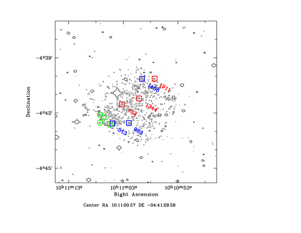
Figure 1: The Sextans A dwarf irregular galaxy. The three A supergiants analyzed in this work are indicated with red squares; other blue supergiants from the target list are indicated with blue squares. The four bright compact H II regions analyzed in Skillman et al. (1989) are shown with green circles.

A complete log of the ESI and UVES observations is found in Tab. 1 together with some additional information on the instrumental configurations used for the individual observations and the environmental conditions during the actual observations. The complete sample of examined Sextans A targets is presented in Tab. 3 together with the radial velocity and spectral type information as obtained either during the detailed analyses of the stars or for the discarded stars during the pre-selection process; the location of the individual targets within the galaxy field is shown in Fig. 1 together with the positions of the four bright compact H II regions analyzed by Skillman et al. (1989).

All UVES data were reduced using the dedicated UVES pipeline which is described by Ballester et al. (2000) and is available as a special package within the ESO-MIDAS data reduction system. Optimum extraction with cosmic rejection and sky subtraction was used to extract the individual stellar spectra. A typical signal-to-noise ratio (SNR) of $\approx 9$ in the wavelength regime corresponding to the $B$ band was obtained for a single spectrum of 4500 sec exposure time. The typically 10 individual spectra per star were then corrected for the spectrograph’s response function to obtain a smooth continuum, rebinned to heliocentric velocities, and eventually combined with additional cosmic clipping. The combined spectra were resampled and rebinned to a 2-pix resolving power of $R=20\,000$ which was used throughout the analyses. The reduced resolving power allows to increase the SNR per resolution element without having to sacrifice line profile information. The projected rotational velocities of the three stars were later determined to be $>30$ km/s, i.e., all line profiles remain fully resolved at the reduced resolution of $15$ km/s. The SNRs obtained for the combined UVES spectra are listed in Tab. 2 for different wavelength regions of interest. The observations of individual stars in a distant Local Group galaxy as presented here are at the limit of the capabilities of today’s largest telescopes and most sensitive spectrographs: despite total integration times of typically 12.5 hrs per star, SNRs of 30 are achieved at best for a resolving power of $R=20\,000$ for a $V=19.5$ mag star which is deemed just sufficient for detailed abundances analyses as will be shown in this work.

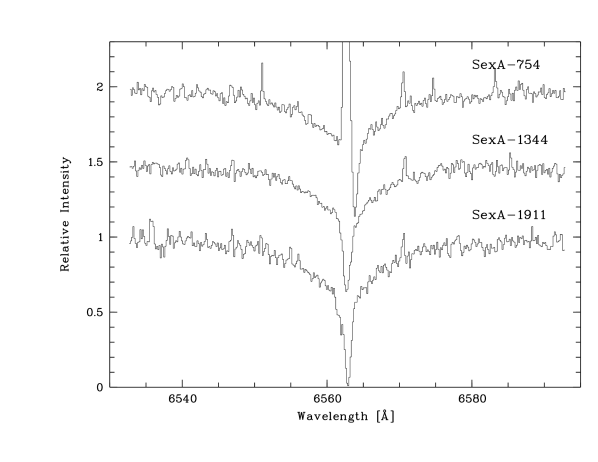
Figure 2: H$\alpha$ profiles of the three Sextans A stars under analysis. All profiles have been shifted to the laboratory wavelength of H$\alpha$ by the respective heliocentric velocties from Tab. 3. The sharp, slightly blue-shifted emission seen in star SexA-754 is due to imperfect subtraction of the highly-structured diffuse H$\alpha$ emission from the H I gas of the galaxy. Note, that no strong wind-emission features are present in the H$\alpha$ profiles indicating the lower luminosity and/or metallicity of the stars.

In Fig. 2 the H$\alpha$ profiles of the three stars are shown. To obtain the stellar line profiles, the contribution of the diffuse H$\alpha$ emission of Sextans A which was found for all stars was subtracted as part of the ’sky’ subtraction in the extraction process of the spectra. Inspecting the raw 2D spectra, the diffuse H$\alpha$ emission does show spatial structure but averaged along the slit its distribution is mostly Gaussian. The diffuse emission is blueshifted by an average of $-10$ km/s with respect to the stellar spectra and consistent with the H I radial velocity of Sextans A (Huchtmeier & Richter, 1986). The average FWHM of the emission is $47$ km/s corresponding to a ($1\sigma$) velocity dispersion of $20$ km/s. This is in excellent agreement with a thermal velocity ($22$ km/s) of a warm interstellar medium if a temperature of $10\,000$ K is assumed.

In the sky-subtracted stellar H$\alpha$ profiles in Fig. 2 no stellar line-emission is visible in H$\alpha$ which indicates that the selected stars are supergiants of lower luminosity. This was already expected from the fact that during the selection process only stars about 2 magnitudes fainter than the brightest blue stars in Sextans A (SexA-513) turned out to be normal A supergiants. Interestingly, no brighter, more extreme A supergiants, which are supposed to be the visually brightest stars, were found in the whole galaxy. The same observation was made during the study of the dIrr WLM (Venn et al., 2003a). The selection process applied to find candidate stars for abundance analyses in Sextans A and WLM was not rigorous enough to exclude that this finding is a selection effect intrinsic to our procedure. However, the lack of luminous A supergiants might as well be an evolution effect due to the low metallicity of the galaxy. Similarly, the lack of wind emission features in H$\alpha$ as seen in Fig. 2 might be due to the low metallicity suppressing the formation of stellar winds due to the reduced radiation line-driving on the metal-poor gas.

Lower-luminosity supergiants as were found in Sextans A are best suited for abundance analyes. Higher-luminosity stars are difficult to analyze because the line-forming regions of their atmospheres are no longer in hydrostatic equilibrium but are found in the acceleration zone of the stellar wind. Further, for lower-luminosity A supergiants, the effects due to intrinsic photospheric and wind variability on the line profiles is negligible (Kaufer et al., 1996). Equivalent width variations of weak ($W_{\lambda}<200$ mÅ) photospheric lines as used for the abundance analyses in this work are found to be $\leq 10$ % (Kaufer et al., 1997).

3 Atmosphere Analyses

The atmosphere analyses of the three stars in Sextans A have been carried out in line with previous analyses of A supergiant stars in the Galaxy (Venn, 1995a, b), the Magellanic Clouds (Venn, 1999), M31 (Venn et al., 2001) and the dwarf irregular galaxies NGC 6822 (Venn et al., 2001) and WLM (Venn et al., 2003a). Maintaining a consistent analysis process across the different studies of A supergiant stars is considered crucial to obtain consistent and comparable abundance results. In particular results from differential analyses can then be considered the most reliable because the uncertainties in the determined absolute elemental abundances shall cancel out at least to some extend.

The atmosphere computations are based on plane parallel, hydrostatic, and line-blanketed ATLAS 9 LTE model atmospheres (Kurucz, 1979, 1988, 1993) which are considered to be appropriate for the photosphere analysis of lower luminosity A supergiants (Przybilla, 2002). To account for the possible effects of the low metallicity of Sextans A on the model atmosphere structure, all atmosphere models have been computed with a metallicity scaled to $1/10$ of solar and a corresponding opacity distribution function. The value of $[{\rm M}/{\rm H}]=-1$ was chosen in agreement with the present day oxygen abundances as derived from the analysis of H II regions (Skillman et al., 1989). However, as has been shown later, the effect of atmosphere models with different metallicities on the derived elemental abundances is typically less than $0.05$ dex, i.e., negligible within the estimated systematic errors.

The analyses has been restricted to the use of weak absorption lines only to minimize the effects of the neglected spherical extension and of the neglected NLTE conditions in these extended, low gravity supergiant stars on the model atmospheres. Further, weak lines are preferred because they suffer less from NLTE and microturbulence effects in the line formation process. Weak lines in this context are defined as lines where a change in the microturbulence $\xi$ of $\Delta\xi=1$ km/s results in a change in the elemental abundance of $\log(X/\rm{H})\leq 0.1$ dex. To fulfill this weak-line condition, the equivalent width of the corresponding line has typically to be $W_{\lambda}<160$ mÅ. Weak-line analyses are a challenge for faint and metal-poor targets as analyzed in this work, in particular if the galaxies are far away, the targets are faint and the SNR of the high-resolution spectra is comparatively low as it is the case here. The absorption lines have been measured by fitting Gaussian profiles to the weak line profiles and to the stellar continuum, the latter being the main source of uncertainty in the derived equivalent widths $W_{\lambda}$. The comparatively low SNR leaves a non-negligible uncertainty of about $10$% in the definition of the continuum level and therefore in the measured $W_{\lambda}$ in the blue part of the combined spectra.

The stellar model atmosphere parameters effective temperature $T_{\rm eff}$, gravity $\log g$, and microturbulence $\xi$ are in the following determined solely from spectral features and therefore are not affected by the (badly-defined) extinction.

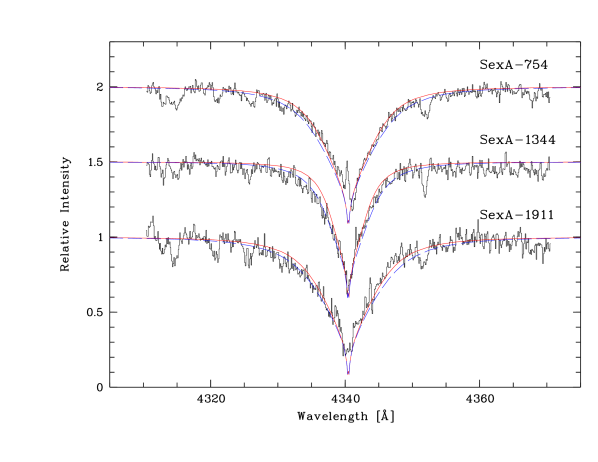
Figure 3: H$\gamma$ profiles of the three Sextans A stars under analysis. The solid (red) line indicates the fit of the synthetic profiles to the wings of the Balmer line for the final model atmosphere parameters while the dashed (blue) line is the synthetic profile for the same stellar parameters but with $\log g$ increased by $+0.2$ dex which is considered the uncertainty in the fit.

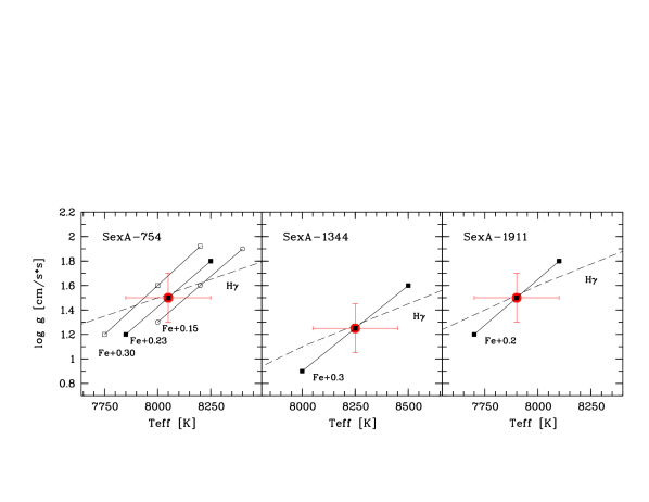
Figure 5: The final selected atmospheric parameters for the three analyzed A supergiants are indicated in the $T_{\rm eff}-\log g$ diagram by the (red) solid circles with errorbars and were determined by fits to the H$\gamma$ profiles (dashed line) and the Fe I/Fe II ionization equilibria (filled squares). In the labels “Fe $x$”, the $x$ notes the NLTE correction applied to the Fe I abundances. For star SexA-754 the ionization equilibria for three different Fe I NLTE corrections are shown to illustrate the effect of the estimated uncertainties on the stellar parameters.

The temperature and gravity parameters of the best fits of synthetic Balmer-line profiles to the gravity-sensitive wings of the H$\gamma$ profiles (see Fig. 3) define a relation in the $T_{\rm eff}$ – $\log g$ plane as shown for each star in Fig. 5. The temperature and gravity parameters for which an ionization equilibrium of Fe I and Fe II is found defines a temperature-sensitive relation in the $T_{\rm eff}$ – $\log g$ plane (for a detailed discussion of the Fe I NLTE corrections see below). The intersection of both relations defines the position in the $T_{\rm eff}$ – $\log g$ plane for which both, the best fit to the H$\gamma$ profile and the ionization equilibrium of Fe I and Fe II are achieved. This parameter pair is adopted as the atmosphere parameters of the star.

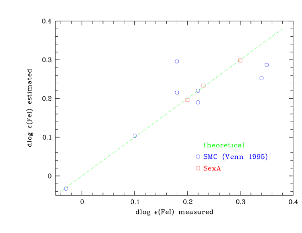
Figure 4: The Fe I NLTE corrections used in this work have been estimated using Eqn. (3). This relation was calibrated for the low metallicity and gravity of the stars in Sextans A (red squares) using the measured NLTE corrections in stars in the SMC (blue circles). The figure compares the measured corrections with the estimates from Eqn. (3).

Due to the low temperature of the analyzed stars and the comparatively low SNR of the combined spectra (cf. Tab. 2) none of the weak spectral lines of Mg II present in the observed spectral ranges could be used to determine the stellar parameters from the most reliable ionization equilibrium of Mg I and Mg II. Also the strong, easy to measure Mg II$\lambda 4481$ line had to be discarded because of its known high sensitivity to NLTE and microturbulence effects: NLTE corrections are of the order of $-0.3$ dex for the temperature and gravities of the stars analyzed here; an uncertainty of the microturbulence of $1$ km/s results in a change of the computed abundances of the same order. Instead, as already described above, the ionization equilibrium of Fe I and Fe II was used in this work. This introduces an additional uncertainty to the determination of the stellar parameters because of the sensitivity of Fe I lines to NLTE effects (Boyarchuk et al., 1985; Gigas, 1986; Rentzsch-Holm, 1996). The NLTE effects on Fe II lines are considered negligible (Rentzsch-Holm, 1996; Becker, 1998). To quantitatively incorporate the dependencies of the Fe I NLTE corrections on temperature, gravity, and metallicity on the Fe I/Fe II ionization equilibrium, the results from Rentzsch-Holm (1996) presented in her Figs. 4 and 5 were used to derive a relation for the NLTE correction to be applied to the Fe I abundances for the limited temperature range of interest in this work, i.e., $7000<T_{\rm eff}<9000$ K:

$$\Delta\log\epsilon_{\rm FeI} = 0.09\frac{T_{\rm eff}[K]}{1000}-0.58$$

$$-2(\log g-4)\left(0.04\frac{T_{\rm eff}[K]}{1000}-0.27\right)$$

$$-0.1[{\rm M}/{\rm H}]$$

$$-{\it 0.28}$$

The first and second terms describe the temperature and gravity dependent NLTE correction as derived for solar metallicity main sequence ($\log g\approx 4.0$) stars. The third term describes the metallicity dependence of the NLTE correction as derived for metallicities in the range $[{\rm M}/{\rm H}]=\pm 0.5$. Due to the considerably lower gravities and metallicities of the stars studied here, this relation has to be used with caution.

To test the relation for stars of lower gravity and metallicity as studied in this work the relation was applied to the data set of A supergiants in the SMC as analyzed by Venn (1999). The stellar parameters of the SMC stars are all based on the most reliable Mg I to Mg II ionization equilibrium. The Fe I NLTE corrections were determined as $\Delta\log\epsilon_{\rm Fe\,I}=\log({\rm Fe\,II/H})-\log({\rm Fe\,I/H})$ assuming that the NLTE corrections for Fe II are negligible (Becker, 1998; Rentzsch-Holm, 1996). It is found that the above relation fits the SMC data well if an additional correction of $-0.28$ is added, cf. Fig. 4. It is important to note that the relation describes rather well all SMC stars with Fe I to Fe II abundance differences over the whole range from $0.0$ to $0.3$ dex. This constant additional (fourth) term in the relation seems sufficient to absorb the additional NLTE effects due to low gravity and low metallicity, at least for the narrow temperature range of $7000-9000$ K, gravities of $\log g\approx 1.5$, and metallicities of $[{\rm M}/{\rm H}]\approx-0.7$, i.e., close to the stellar parameters of the stars studied in Sextans A. In the subsequent atmosphere analysis, the final stellar parameters for the Sextans A stars were chosen to be consistent with the Fe I NLTE corrections as given by the above relation. The adopted final corrections are $+0.23$ dex for SexA-754, $+0.30$ dex for SexA-1344, and $+0.20$ dex for SexA-1911 and are shown in Fig. 4, too. It should be further noted that the remaining uncertainty of $\pm 0.1$ dex in the Fe I NLTE corrections has been taken into account in the overall error budget as estimated from the uncertainties of the determination of the stellar parameters (cf. below).

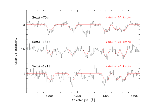
Figure 6: Spectrum synthesis to determine the projected rotational velocity $v\sin i$ of the three stars. The lines of Ti II$\lambda\lambda 4290,4294,4300,4301$ and the Fe II$\lambda 4303$ line where used to fit the profiles. Due to the lower $v\sin i$ of SexA-1344, the Fe II$\lambda 4297$ line could be added to the list of lines to be fitted.

Microturbulence $\xi$ has been determined from the line abundances of the numerous lines of different strength from the ions Fe II, Ti II, and Cr II. A single value of $\xi$ for each star was adopted so that no trend of the computed elemental abundance is found with the equivalent width of the lines within the uncertainty of $\Delta\xi=1$ km/s. The estimated uncertainties in $T_{\rm eff}$ are dominated by the uncertainties of the derived Fe I NLTE corrections but also have to account for the uncertainties of the assumption of negligible NLTE effects on Fe II in the ionization equilibrium used for the temperature determination. The effect of a change of the Fe I NLTE correction of $\pm 0.08$ dex (as derived from the residuals in Fig. 4) is shown in Fig. 5 for star SexA-754. If we assume an uncertainty of $\pm 0.05$ dex for the LTE assumption for Fe II, we obtain an estimate for the total uncertainty of $\pm 0.1$ dex which translates into $\Delta T_{\rm eff}=\pm 200$ K as indicated by the horizontal errorbars in Fig. 5. Uncertainties in gravity are estimated to $\Delta\log g=\pm 0.2$ dex from varying the fits to H$\gamma$ for different $\log g$ at constant $T_{\rm eff}$. The resulting change of the synthetic profile for a variation of $\Delta\log g=+0.2$ dex is shown in Fig. 3. With the determined stellar parameters and elemental abundances (cf. below), a small section of the spectrum between $4285-4305$ Å was synthesized to determine the projected rotational velocities $v\sin i$ of the three stars. This spectral region contain several stronger and isolated Ti II and Fe II lines. For a given resolving power of $R=20\,000$ or $15$ km/s and the given heliocentric radial velocities of the stars the respective values of $v\sin i$ were obtained by least-square fitting of the synthetic line profiles to the observed spectra while keeping the elemental abundances for the metal lines fixed to the value determined before. The resulting fits are shown in Fig. 6 and the corresponding values for $v\sin i$ are reported in Tab. 4.

The spectral types of the three stars were defined according to their effective temperatures according to Schmidt-Kaler (1982). It should be noted that this spectral classification does not take into account any metallicity dependence of the classification criteria but is based on stars of solar metallicities. The luminosities of the three stars were then derived from the visual magnitudes as given in Tab. 3 using the distance modulus of $\mu_{0}=25.6$ from Dolphin et al. (2003a) and the (close to zero) bolometric corrections from Schmidt-Kaler (1982) corresponding to the spectral types. The resulting spectral types and luminosities are given in Tab. 4 together with the stellar radii as computed from the luminosity and the effective temperature. The luminosities of all three stars are consistent with the evolutionary track of a $12\,{\rm M}_{\odot}$ star (Lejeune & Schaerer, 2001), i.e., a ZAMS mass compatible with evolved low-luminosity A supergiants. This finding further confirms the Sextans A membership of the three analyzed supergiant stars.

4 Abundances

The list of appropriate spectral lines for the abundance determinations and the corresponding atomic data were adopted from the previous analyses of Venn (1995a, b, 1999); Venn et al. (2001). Atomic data and the abundances derived from the individual lines are listed in Tab. 6 together with the measured equivalent widths $W_{\lambda}$. All abundance calculations in LTE/NLTE and LTE spectrum synthesis have been carried out using a modified version of the LINFOR code. The resulting average elemental abundances are given for each ionization stage in Tab. 4. For each abundance, two error estimates are given, first the r.m.s. line-to-line scatter, second (in italic) the estimated systematic error in the elemental abundance from the uncertainties in the atmospheric parameters $T_{\rm eff}$, $\log g$, and $\xi$. The systematic errors of the average abundances have been estimated by the variation of the individual stellar atmosphere parameters within their estimated uncertainties while keeping the other parameters fixed. The individual error estimates are reported in Tab. 5. From the error estimates it can be seen that Si II, Ti II, Cr II, and Fe II provide the most reliable elemental abundances. However, abundances derived from the Si II ion have been found to suffer from a large spread if derived from stars over a wider range in stellar parameters. The sample of 10 A supergiants in the SMC as analyzed by Venn (1999) shows a spread in the silicon abundances of $\approx 0.5$ dex probably due to neglected NLTE effects in the line formation of the Si II ion. The three stars analyzed here show very consistent silicon abundances because the stellar parameters of the stars are very close to each other. However, since the absolute abundance probably is affected from the uncertainties that were found in other analyses, the abundances from Si II will not be considered in the further discussion of $\alpha$ element abundances.

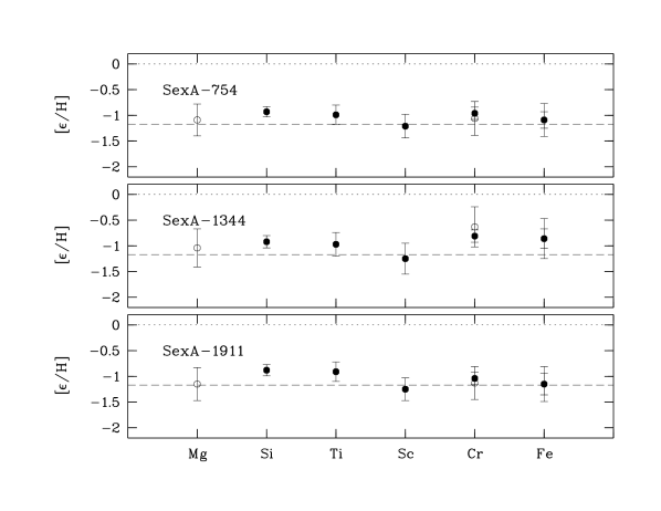
Figure 7: Elemental abundances for SexA-754 (top), SexA-1344 (middle), and SexA-1911 (bottom) relative to solar (dotted line) and to the nebular oxygen underabundance of $-1.17$ dex (dashed line). Abundances derived from neutral atoms are indicated with open circles, abundances from singly ionized atoms with filled circles. The shown errorbars are the estimated combined errors from the uncertainties of the determination of the stellar parameters (cf. Tab. 5).

The average elemental abundances relative to the solar abundances are shown for the three stars in Fig. 7 with the error bars representing the estimated combined systematic errors in the abundances. The combined errors were computed as the quadratic sum of the individual errors from Tab. 5.

The abundances reported for Mg I and Mg II have been computed using NLTE lineformation based on the model atom by Gigas (1988) which delivers results in good agreement with the model atom developed by Przybilla et al. (2001). The NLTE corrections for the individual Mg lines are listed in Tab. 7 and are found to be small and of the order of $\pm 0.1$ dex. Abundances from the strong Mg II$\lambda 4481$ line blend were derived from fits to the observed line profile using spectrum synthesis in LTE; the results are reported in Tab. 6. The NLTE corrections for this line are expected to be large (Przybilla et al., 2001) and very sensitive to the stellar parameters and in particular to the microturbulence (Przybilla, 2003). Therefore, no attempt was made to compute the NLTE corrections and the line was not used for this analysis but is given for reference only.

For star SexA-754, useful upper limits for the equivalent widths of the weak Mg II lines could be given because of the higher SNR of the combined spectrum of this star. The resulting upper limits for the Mg II abundances are consistent with the abundances derived from the Mg I lines and therefore further support the stellar parameters as derived from the Fe I to Fe II ionization equilibrium.

The $\alpha$ element of highest interest is oxygen. Unfortunately, none of the O I lines in the 615 nm and 645 nm spectral regions could be measured in the combined UVES spectra of moderate SNR because of the weakness of the lines at the metallicity of Sextans A. For $[{\rm O/H}]\approx-1$, all O I lines in this spectral region are expected to have equivalent widths of $<20$ mÅ, i.e., clearly below the detection limit of the spectra. However, the low metallicity of Sextans A brings the near-infrared O I$\lambda\lambda 7771$-$7775,8446$ lines of multiplet 1 and 4 into the weak-line regime possibly suited for abundances analyses despite their known high sensitivity to NLTE effects (Przybilla et al., 2000).

Spectra of the respective wavelength regions are only available for one of the stars, SexA-754. Since the near-infrared lines are non-resolved multiplets, fitting of synthetic LTE line profiles was used to determine LTE oxygen abundances (see Fig. 8). The oxygen abundances measured in LTE are $12+\log{\rm{O/H}}=9.1\pm 0.3$ for O I$\lambda 7771$-$7775$ and $12+\log{\rm{O/H}}=8.1\pm 0.3$ for O I$\lambda 8446$. Detailed computations of the NLTE corrections for the given stellar parameters of SexA-754 at the metallicity of Sextans A will be required before accurate oxygen abundances can be derived for this star. In any case, the expected uncertainties will remain large, first because of the large required deviations from LTE to bring the oxygen abundances into the reasonable range of $12+\log{\rm{O/H}}\approx 7.8$ (assuming an underabundance of $[\alpha/{\rm H}]=-1.0$ as suggested from the other $\alpha$ elements silicon and magnesium), second because of the low quality of the near-infrared spectra, which results in a non-negligible uncertainty in the continuum definition, which is crucial for an accurate line profile modeling. The estimated error in the derived LTE abundances of $\pm 0.3$ dex is due to this uncertainty in the continuum localization. Therefore, currently no further attempt has been made to determine the NLTE corrections for the near-infrared lines of SexA-754. In the following, elemental abundances derived from Mg I will be used instead for the discussion of $\alpha$ element abundances in Sextans A. Earlier studies in the SMC (Venn, 1999) and NGC 6822 (Venn et al., 2001) have shown that a good agreement between the $\alpha$ elements oxygen and magnesium is found for different stars and so both elements may be used to represent the $\alpha$ elemental abundance of the star. The average $\alpha$ element abundance of the three stars in Sextans A are found to be $\left<[{\rm Mg\,I/H}]\right>=-1.09\pm 0.02\pm{\it 0.19}$ which is in excellent agreement with the $\alpha$ element abundances from the H II regions of $[\rm{O/H}]=-1.17$ as derived by Skillman et al. (1989) and the recently revised value $[\rm{O/H}]=-0.95$ of Pilyugin (2001).

The iron-group elemental abundances of the three stars are in excellent agreement as derived from lines of Cr I, Cr II, Fe I, and Fe II. The good agreement of the abundances from the two different ionization stages of chromium is a further indication for correct stellar parameter. However, it should be noted that this equilibrium is based on a single Cr I line. Possible NLTE effects on this line which were not taken into account in the abundance computation appear therefore to be small. The agreement of the Fe I and Fe II abundances and hence the ionization equilibrium is achieved if the respective Fe I NLTE corrections are applied, i.e., $+0.23$ dex for SexA-754, $+0.30$ dex for SexA-1344, and $+0.20$ dex for SexA-1911. As discussed before, the determination of the stellar parameter is based specifically on this NLTE corrected ionization equilibrium. The abundances of Fe II and Cr II have been derived from numerous lines and are regarded as the most reliable: the dependency of the abundances on the stellar parameters is small (cf. Tab. 5) and possible NLTE effects on these dominant ionization stages are expected to be small.

The mean metallicity of the three stars are so found to be $\left<[({\rm Fe\,II,Cr\,II})/{\rm H}]\right>=-0.99\pm 0.04\pm{\it 0.06}$ which — to our knowledge — makes these three stars the to date most metal-poor massive stars in any galaxy for which a detailed abundance analysis has been carried out.

Titanium and scandium can be considered as either $\alpha$ or iron-group elements. The Ti abundances were derived from a large number of lines of the dominant ionization stage of singly ionized titanium and are in good agreement with iron, i.e., $\left<[{\rm Ti\,II}/{\rm Fe\,II}]\right>=0.08\pm 0.05\pm{\it 0.08}$ while Sc shows a slight underabundance of $\left<[{\rm Sc\,II}/{\rm Fe\,II}]\right>=-0.20\pm 0.03\pm{\it 0.09}$. This might be due to the smaller number of available lines and higher temperature sensitivity of Sc II. Furthermore, the hyperfine-structure terms in the lines of odd elements of the iron group due the presence of a nuclear magnetic moment have been neglected. Due to these uncertainties, no further discussion of the scandium abundances will follow.

5 Discussion

For the first time, the present-day iron group abundances have been determined from stars in Sextans A. The mean underabundance relative to solar is $\left<[{\rm Fe/H}]\right>=-1.03\pm 0.05\pm{\it 0.11}$ and has been derived from the Fe II abundances which are expected to be the most reliable. This result is well supported by abundances measured for a second iron-group element, namely Cr II with a mean underabundance of $\left<[{\rm Cr\,II/H}]\right>=-0.94\pm 0.06\pm{\it 0.07}$. The individual iron-group abundances of the three stars from which the mean abundances were computed are in good agreement within the estimated systematic errors.

The star formation history of Sextans A derived by Dolphin et al. (2003b, and references therein), suggests that the metallicity reached $[{\rm M}/{\rm H}]=-1.1\pm 0.2$ only 2 Gyr ago. The metallicity spread of $\pm 0.2$ dex is to account for the dispersion in the Blue Helium Burning (BHeB) stars. The mean stellar metallicity found here from iron and chromium, $\left<[({\rm Fe\,II,Cr\,II})/{\rm H}]\right>=-0.99\pm 0.04\pm{\it 0.06}$, is consistent with the CMD stellar populations analysis.

The mean $\alpha$ element abundance from magnesium in the three stars is $\left<[\alpha({\rm Mg\,I})/{\rm H}]\right>=-1.09\pm 0.02\pm{\it 0.19}$ which is in good agreement with the nebular results for oxygen, $[\rm{O/H}]=-1.17$ (Skillman et al., 1989) and $[\rm{O/H}]=-0.95$ (Pilyugin, 2001). It is worth noting that this independent measurement of the $\alpha$ elemental abundance confirms the location of Sextans A in the fundamental metallicity – luminosity relationship for dwarf galaxies (Skillman et al., 1989; Richer & McCall, 1995).

The agreement between the $\alpha$ element abundances from A supergiant stars and the nebular abundances is as expected. These stars have ages $\approx 10^{7}$ Myr and are expected to have formed out of the same interstellar gas as seen in the nebulae. Similar findings are reported from the abundance analyses of B-type main sequence stars in Orion and the LMC (Cunha & Lambert, 1994; Korn et al., 2002), respectively, the Galactic abundance gradients from B stars (Gummersbach et al., 1998; Rolleston et al., 2000), and A supergiant analyses in the SMC, M31, and NGC 6822 (Venn, 1999; Venn et al., 2000, 2001), respectively. It should be noted here, that the pristine nebular and stellar abundances of some elements can be altered by effects of dust depletion and rotational mixing which complicates a quantitative comparison of nebular and stellar abundances (Korn et al., 2002). However, in the case of the stars and nebulae studied in Sextans A , the good agreement within the estimated errors suggest that the contributions due to these effects to the determined abundances are small. Only the dIrr galaxy WLM shows a discrepancy between the stellar and nebular $\alpha$ element abundances (Venn et al., 2003a). The nebulae in WLM have $[{\rm O}/{\rm H}]=-0.89$ (Skillman et al., 1989), whereas two A supergiants have $[{\rm Mg}/{\rm H}]=-0.62$, and one star suggests $[{\rm O}/{\rm H}]=-0.21$. These are significant differences that are currently not understood and may suggest that WLM is the first galaxy to display inhomogeneous mixing.

The spatial distribution of abundances in a galaxy keeps an important record of the re-distribution history of freshly produced elements and their mixing with the ISM. As can be seen from Fig. 1, the three stars analyzed in this work and the four bright compact H II regions examined by Skillman et al. (1989) lie on a line across the central, visually brightest part of the galaxy. Adopting D${}_{\rm Sex\,A}=1.3$ Mpc (Dolphin et al., 2003a), no significant $\alpha$ element abundance variations are found over a distance of $0.8$ kpc as covered by the stars (between SexA-754 to SexA-1344 to SexA-1911), and over $1.6$ kpc if the H II regions are included. The same level of abundance homogeneity is found for the iron-group elements in the stars. The high level of homogeneity of nebular abundances in dwarf irregular galaxies has been discussed as possible evidence against in situ (“on the spot”) enrichment by Kobulnicky & Skillman (1997) and therefore against the general validity of the instantaneous recycling approximation as typically used in chemical evolution models. Kobulnicky & Skillman (1997) favour a scenario in which the newly synthesized elements remain in either a difficult to observe hot $10^{6}$ K or an equally difficult to observe cold, dusty phase while mixing throughout the galaxy. Recent Chandra spectroscopy results for NGC 1569 by Martin, Kobulnicky, & Heckman (2002) favor the hot phase as the reservoir for newly synthesized and expelled gas.

The $\alpha/{\rm Fe}$ abundance ratio is a key constraint for the chemical evolution of a galaxy. $\alpha$ elements are primarily synthesized in SNe II while the iron-group elements are mainly produced in SNe Ia but also in SNe II. A star formation burst in a galaxy will temporarily increase the $\alpha/{\rm Fe}$ ratio of the ISM due to the massive stars that quickly enrich the ISM with $\alpha$ elements, while the lower mass stars will then slowly increase the content of iron-group elements resulting in a slow decline of the $\alpha/{\rm Fe}$ ratio of the galaxy (Tinsley, 1979). Gilmore & Wyse (1991) demonstrated the expected differences in the $\alpha/{\rm Fe}$ ratios for galaxies with different star formation histories, and in particular noted that the solar $\alpha/{\rm Fe}$ ratio must not be regarded as an universal ratio.

From the three stars in Sextans A, the $\alpha/{\rm Fe}$ ratio is measured as $\left<[\alpha({\rm Mg\,I})/{\rm Fe\,II,Cr\,II}]\right>=-0.11\pm 0.02\pm{\it 0.10}$. This $\alpha$/Fe ratio is much lower than in Galactic stars of similar metallicity (Edvardsson et al., 1993; Nissen & Schuster, 1997). At the metallicity of these Sextans A stars, [Fe/H] $\approx-1$, the Galactic thick disk and Galactic halo stars overlap with a [$\alpha$/Fe] $\approx$ +0.3. The lower $\alpha$/Fe ratios in these Sextans A stars further follows the trend found from the abundance analyses of stars in two other dIrrs, NGC 6822 and WLM (Venn et al., 2001, 2003a), but extends the metallicity range now sampled from $[{\rm Fe}/{\rm H}]=-0.5$ in those galaxies to $[{\rm Fe}/{\rm H}]=-1.0$. As discussed by Venn et al. (2003a), this lower metallicity now overlaps the upper metallicities sampled by red giant stars in dwarf spheroidal galaxies, which also show much lower $\alpha$/Fe ratios than Galactic metal-poor stars (Shetrone et al., 2001, 2003; Tolstoy et al., 2003). In the dwarf spheroidal galaxies, the low [$\alpha$/Fe] ratios near [Fe/H] = $-1.0$ are most likely due to the lower star formation rates, thus slower chemical evolution. The metallicity range of the dwarf irregular galaxies also overlaps with the damped Ly$\alpha$ absorption systems (Nissen et al., 2003; Ledoux et al., 2002; Pettini et al., 1999), which are also recognized to have low $\alpha$/Fe ratios. This might suggest that low $\alpha$/Fe ratios are a generic effect at low metallicities.

The star formation histories for Sextans A, WLM, and NGC 6822 are globally similar as derived from their CMDs. A comparison can be seen in Fig. 8 of Mateo (1998). Accordingly, all three dIrrs had significant star formation at ancient times, $>5-10$ Gyr ago, with a hiatus at intermediate ages, $1-5$ Gyr ago, and recent star formation events in the past 1 Gyr. Matteucci (2003) has recently emphasized that the SFH of a galaxy affects the absolute elemental abundances, but is only of minor importance for the abundance ratios, the latter being primarily determined by the stellar lifetimes, initial mass functions (IMF) and the stellar nucleosynthesis. Thus, the impact of different SFHs on the $\alpha/{\rm Fe}$ ratio is related to the star formation efficiency, and manifests itself as a short plateau in the $[\alpha/{\rm Fe}]$ ratio at low metallicities in galaxies with low star formation rates, like irregulars (either in bursts or continuous), while the plateau is maintained to higher metallicities for systems with high star formation rates like bulges and ellipticals. Thus, our finding that the [$\alpha/{\rm Fe}$] ratios in three dIrrs with similar SFHs is significantly lower than in the metal-poor Galactic stars can be explained in this scenario. The three dIrrs with a metallicity range from $-1<[{\rm Fe}/{\rm H}]<-0.4$ have already left the $[\alpha/{\rm Fe}]$ plateau and presently display the same lower $[\alpha/{\rm Fe}]$ ratio. That this ratio is similar to solar suggests that the integrated stellar yields from a star formation event is consistent with the solar abundance ratios, probably due to the universal nature of stellar lifetimes, IMFs, and stellar nucleosynthesis. That the high-redshift DLA absortion systems also show low [$\alpha$/Fe] ratios suggests that they are also systems with low star formation rates, but this could be either irregular galaxies or the outer parts of spirals. A recent study of published DLA system abundances in comparison with chemical evolution models of different galaxy morphologies by Calura et al. (2003) has identified the irregular and spiral galaxies as the possibly ideal sites to create the DLA systems, while ellipticals can be ruled out.

The value of high resolution spectroscopy of the brightest blue stars in nearby galaxies for detailed, quantitative abundance studies has been further demonstrated in this work. To gain further insight into the chemical evolution of the dwarf galaxies and hence into the early evolution of galaxies with low star formation rates, requires more detailed abundance analyses of their stars, particularly towards the lower metallicities.

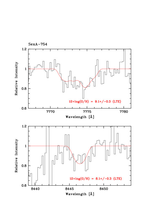
Figure 8: Spectrum synthesis for the the near-infrared O I$\lambda\lambda 7771$-$5,8446$ multiplet lines. The oxygen abundance was fitted using spectrum synthesis in LTE. The uncertainty of the LTE abundances of $\pm 0.3$ dex are due to the badly-defined continuum. To convert the measured LTE abundances into sensible oxygen abundances detailed computation of the expectedly large NLTE corrections (Przybilla et al., 2000) have to be carried out (see Section 4).

Table 1: Sextans A Keck/ESI and VLT/UVES observations

Star	Date	UTC	$\lambda_{\rm c}$	Exp.Time	Airmass	Seeing
		Start	[nm]	[sec]	Start	[$\arcsec$]
Keck/ESI
SexA-513	2002-02-13	08:45	750	2700	1.30	1.5
	2002-02-14	07:49	750	2700	1.38	1.6
SexA-983	2002-02-13	09:44	750	3600	1.15	1.5
SexA-1344	2002-02-14	09:59	750	3600	1.10	1.6
SexA-1456	2002-02-13	11:02	750	2600	1.10	1.5
VLT/UVES
SexA-754	2002-01-11	04:45	390+580	4500	1.39	0.98
	2002-01-13	05:55	390+580	4500	1.14	1.50
	2002-01-13	07:12	390+580	4500	1.06	1.20
	2002-01-18	04:55	390+580	4500	1.24	1.25
	2002-01-20	07:17	390+580	4500	1.06	0.97
	2002-01-23	05:55	390+580	4500	1.08	0.81
	2002-02-08	02:00	390+580	4500	1.80	1.19
	2002-02-09	02:32	390+580	4500	1.50	0.73
	2002-02-10	01:55	390+580	4500	1.77	0.75
	2002-02-11	02:41	390+580	4500	1.40	0.58
	2002-02-12	02:14	390+580	4500	1.55	1.13
	2002-04-14	00:58	437+840	4500	1.07	1.00
	2002-04-14	02:15	437+840	4500	1.08	1.02
	2002-04-15	00:30	437+840	4500	1.08	0.80
	2002-04-15	01:48	437+840	3600	1.07	0.67
	2002-04-15	02:50	437+840	3600	1.14	0.87
	2002-04-15	03:51	437+840	3600	1.33	1.01
SexA-1344	2002-12-30	05:19	390+580	4500	1.48	1.25
	2002-12-30	06:36	390+580	4500	1.17	1.03
	2003-01-01	07:24	390+580	4500	1.08	1.42
	2003-01-08	04:39	390+580	4500	1.50	0.84
	2003-01-08	05:58	390+580	4500	1.18	1.08
	2003-01-08	07:16	390+580	4500	1.07	0.61
	2003-02-04	03:12	390+580	4500	1.39	1.00
	2003-02-04	04:29	390+580	4500	1.14	1.27
	2003-02-04	05:46	390+580	4500	1.06	1.15
	2003-02-05	04:38	390+580	4500	1.12	1.29
SexA-1911	2003-01-12	04:58	390+580	4500	1.32	1.19
	2003-02-05	05:59	390+580	4500	1.06	1.02
	2003-02-05	07:19	390+580	4500	1.14	1.17
	2003-02-06	03:43	390+580	4500	1.23	0.93
	2003-02-07	04:13	390+580	4500	1.15	0.78
	2003-02-07	05:29	390+580	4500	1.06	0.95
	2003-02-07	07:49	390+580	4500	1.23	0.93
	2003-02-08	04:07	390+580	4500	1.15	1.22
	2003-02-08	06:22	390+580	4500	1.08	1.09
	2003-02-08	07:40	390+580	4500	1.21	0.94
SexA-513	2002-04-13	23:19	390+580	1800	1.23	1.12
	2002-04-14	23:23	390+580	1800	1.21	0.91
	2002-04-14	00:12	390+580	1800	1.14	0.72
SexA-983	2002-04-13	23:53	390+580	3600	1.15	1.13

Note. — All ESI data was taken in echelle mode with a $20\arcsec\times 1.25\,\arcsec$ slit corresponding to a resolving power of $R=3200$. The wavelength coverage is $390-1100$ nm. All UVES data was taken in dichroic mode, with a $1.2\,\arcsec$ slit width and 2x2 CCD binning corresponding to a 3-pix resolving power of $R=40\,000$. The wavelength coverage of the dichroic settings is for 390+580: $330-452,\ 478-575,\ 584-680$ nm and for 437+840: $376-498,\ 650-831,\ 845-1025$ nm.

Table 2: Signal-to-Noise Ratios of the combined UVES spectra

Star	Signal-to-Noise Ratio
	@400 nm	@500 nm	@650 nm	@800 nm
SexA-754	35	45	35	10
SexA-1344	30	35	30	$\cdots$
SexA-1911	25	35	25	$\cdots$
SexA-513	30	35	30	$\cdots$
SexA-983	15	20	15	$\cdots$

Table 3: Sextans A sample

Star	$V$	$(B-V)$	RVhel[km/s]	Sp.Type	Comment
analyzed targets
SexA-754	$19.5$	$-0.014$	$+340$	A7 Iab supergiant	UVES (cand. 2)
SexA-1344	$19.4$	$-0.083$	$+320$	A7 Iab supergiant	ESI+UVES (cand. 4)
SexA-1911	$19.6$	$-0.004$	$+320$	A8 Iab supergiant	UVES (cand. 5)
discarded targets
SexA-513	$17.5$	$-0.031$	$+350$	F hypergiant	ESI+UVES (cand. 1)
SexA-983	$18.3$	$-0.011$	$+290$	G supergiant	ESI+UVES (cand. 3)
SexA-1456	$18.8$	$+0.254$	$+320$	K supergiant	ESI (cand. 6)

Table 4: Atmospheric Analysis

	Solar	SexA-754	SexA-1344	SexA-1911
$T_{\rm eff}$ [K]		$8050\pm 200$	$8250\pm 200$	$7900\pm 200$
$\log g$ [cm/s2]		$1.5\pm 0.2$	$1.25\pm 0.2$	$1.5\pm 0.2$
$\xi_{\rm micro}$ [km/s]		$4.0\pm 1$	$3.5\pm 1$	$3.5\pm 1$
$v\sin i$ [km/s]		$50\pm 5$	$35\pm 5$	$45\pm 5$
$\log(L/{\rm L}_{\odot})$		$4.35\pm 0.2$	$4.39\pm 0.2$	$4.31\pm 0.2$
$R/{\rm R}_{\odot}$		$77\pm 20$	$77\pm 20$	$76\pm 20$
Sp.Type		A7 Iab	A7 Iab	A8 Iab
Mg I (NLTE)	$7.58$	$6.49\pm 0.01\ (4)\pm{\it 0.30}$	$6.54\pm 0.04\ (4)\pm{\it 0.34}$	$6.43\pm 0.05\ (4)\pm{\it 0.31}$
Mg II (NLTE)	$7.58$	$<6.62\pm 0.18\ (4)\pm{\it 0.07}$	$\cdots$	$\cdots$
Si II (LTE)	$7.56$	$6.63\pm 0.13\ (9)\pm{\it 0.10}$	$6.64\pm 0.08\ (9)\pm{\it 0.12}$	$6.68\pm 0.09\ (9)\pm{\it 0.11}$
Ti II (LTE)	$4.94$	$3.95\pm 0.16(37)\pm{\it 0.19}$	$3.97\pm 0.12(30)\pm{\it 0.23}$	$4.03\pm 0.17(30)\pm{\it 0.19}$
Sc II (LTE)	$3.10$	$1.89\pm 0.06\ (6)\pm{\it 0.23}$	$1.85\pm 0.07\ (4)\pm{\it 0.29}$	$1.85\pm 0.05\ (5)\pm{\it 0.22}$
Cr I (LTE)	$5.69$	$4.63\pm 0.14\ (3)\pm{\it 0.31}$	$5.06\pm 0.00\ (1)\pm{\it 0.37}$	$4.56\pm 0.00\ (1)\pm{\it 0.31}$
Cr II (LTE)	$5.69$	$4.73\pm 0.13(20)\pm{\it 0.12}$	$4.88\pm 0.07\ (8)\pm{\it 0.12}$	$4.65\pm 0.12(13)\pm{\it 0.11}$
Fe I (LTE)	$7.50$	$6.18\pm 0.13(15)\pm{\it 0.31}$	$6.34\pm 0.06\ (7)\pm{\it 0.37}$	$6.15\pm 0.04(12)\pm{\it 0.33}$
Fe II (LTE)	$7.50$	$6.41\pm 0.12(14)\pm{\it 0.16}$	$6.64\pm 0.05(15)\pm{\it 0.19}$	$6.35\pm 0.06(12)\pm{\it 0.21}$

Table 5: Abundance Uncertainties

	SexA-754			SexA-1344			SexA-1911
	$\Delta T_{\rm eff}$	$\Delta\log g$	$\Delta\xi$	$\Delta T_{\rm eff}$	$\Delta\log g$	$\Delta\xi$	$\Delta T_{\rm eff}$	$\Delta\log g$	$\Delta\xi$
	$+200$ K	$+0.2$	$+1$ km/s	$+200$ K	$+0.2$	$+1$ km/s	$+200$ K	$+0.2$	$+1$ km/s
$\Delta\log(X/{\rm H})$
Mg I	$+0.28$	$-0.10$	$-0.10$	$+0.33$	$-0.16$	$-0.05$	$+0.27$	$-0.10$	$-0.15$
Mg II	$+0.01$	$+0.02$	$-0.07$	$+0.06$	$-0.04$	$-0.29$	$+0.03$	$+0.00$	$-0.26$
Si II	$-0.01$	$+0.02$	$-0.10$	$+0.00$	$+0.02$	$-0.12$	$+0.01$	$+0.02$	$-0.11$
Ti II	$+0.18$	$+0.02$	$-0.06$	$+0.21$	$-0.04$	$-0.08$	$+0.17$	$+0.02$	$-0.09$
Sc II	$+0.22$	$+0.00$	$-0.05$	$+0.28$	$-0.08$	$-0.05$	$+0.20$	$+0.00$	$-0.09$
Cr I	$+0.31$	$-0.10$	$-0.01$	$+0.36$	$+0.16$	$-0.02$	$+0.31$	$-0.08$	$-0.03$
Cr II	$+0.11$	$+0.02$	$-0.04$	$+0.11$	$-0.02$	$-0.04$	$+0.11$	$+0.02$	$-0.03$
Fe I	$+0.30$	$-0.10$	$-0.06$	$+0.35$	$+0.16$	$-0.08$	$+0.30$	$-0.08$	$-0.13$
Fe II	$+0.12$	$+0.02$	$-0.11$	$+0.12$	$-0.02$	$-0.15$	$+0.13$	$+0.02$	$-0.16$

Table 6: Line Strengths, Atomic Data and Abundances

	$\lambda$	Multiplet	$\chi$		SexA-754		SexA-1344		SexA-1911
Element	(Å)	Table	(eV)	$\log(gf)$	$W_{\lambda}$	$\log(\epsilon)$	$W_{\lambda}$	$\log(\epsilon)$	$W_{\lambda}$	$\log(\epsilon)$
O I LTE line profile synthesis
$800$	$7772.20$	$1$	$9.15$	$0.37$
$800$	$7774.17$	$1$	$9.15$	$0.22$	700	$9.1$	$\cdots$	$\cdots$	$\cdots$	$\cdots$
$800$	$7775.39$	$1$	$9.15$	$0.00$
$800$	$8846.25$	$4$	$9.52$	$-0.46$
$800$	$8846.36$	$4$	$9.52$	$0.24$	385	$8.1$	$\cdots$	$\cdots$	$\cdots$	$\cdots$
$800$	$8846.76$	$4$	$9.52$	$0.01$
Mg I NLTE
$1200$	$3829.360$	$3$	$2.71$	$-0.21$	$140$	$6.50$	$80$	$6.49$	$140$	$6.42$
$1200$	$5167.320$	$2$	$2.71$	$-0.86$	$75$	$6.49$	$35$	$6.54$	$85$	$6.40$
$1200$	$5172.680$	$2$	$2.71$	$-0.38$	$135$	$6.50$	$80$	$6.58$	$150$	$6.50$
$1200$	$5183.600$	$2$	$2.72$	$-0.16$	$160$	$6.49$	$100$	$6.55$	$160$	$6.38$
Mg II NLTE
$1201$	$3848.210$	$5$	$8.86$	$-1.56$	$<20$	$<6.84$	$\cdots$	$\cdots$	$\cdots$	$\cdots$
$1201$	$4390.570$	$10$	$10.0$	$-0.50$	$<20$	$<6.52$	$\cdots$	$\cdots$	$\cdots$	$\cdots$
$1201$	$7877.050$	$8$	$10.0$	$0.39$	$<60$	$<6.69$	$\cdots$	$\cdots$	$\cdots$	$\cdots$
$1201$	$7896.370$	$8$	$10.0$	$0.65$	$<60$	$<6.43$	$\cdots$	$\cdots$	$\cdots$	$\cdots$
Mg II LTE line profile synthesis
$1201$	$4481.13$	$4$	$8.86$	$0.73$
$1201$	$4481.15$	$4$	$8.86$	$-0.57$	$240$	$5.94$	$200$	$6.10$	$200$	$6.08$
$1201$	$4481.33$	$4$	$8.86$	$0.57$
Si II LTE
$1401$	$3853.660$	$1$	$6.86$	$-1.60$	$50$	$6.48$	$50$	$6.48$	$50$	$6.51$
$1401$	$3856.020$	$1$	$6.86$	$-0.65$	$150$	$6.68$	$140$	$6.74$	$140$	$6.66$
$1401$	$3862.590$	$1$	$6.86$	$-0.90$	$120$	$6.59$	$115$	$6.66$	$115$	$6.60$
$1401$	$4128.050$	$3$	$9.84$	$0.31$	$80$	$6.83$	$70$	$6.69$	$70$	$6.78$
$1401$	$4130.890$	$3$	$9.84$	$0.46$	$70$	$6.56$	$75$	$6.62$	$75$	$6.70$
$1401$	$5041.020$	$5$	$10.07$	$0.17$	$35$	$6.65$	$40$	$6.64$	$40$	$6.81$
$1401$	$5055.980$	$5$	$10.07$	$0.44$	$50$	$6.65$	$50$	$6.57$	$50$	$6.71$
$1401$	$6347.090$	$2$	$8.12$	$0.23$	$140$	$6.76$	$125$	$6.72$	$125$	$6.68$
$1401$	$6371.370$	$2$	$8.12$	$-0.08$	$80$	$6.45$	$95$	$6.67$	$95$	$6.65$
Sc II LTE
$2101$	$4246.820$	$7$	$0.32$	$0.24$	$140$	$1.89$	$100$	$1.87$	$140$	$1.86$
$2101$	$4314.080$	$15$	$0.62$	$-0.10$	$75$	$1.84$	$40$	$1.75$	$80$	$1.77$
$2101$	$4320.730$	$15$	$0.61$	$-0.21$	$80$	$1.99$	$40$	$1.86$	$80$	$1.88$
$2101$	$4325.000$	$15$	$0.60$	$-0.44$	$50$	$1.91$	$\cdots$	$\cdots$	$60$	$1.89$
$2101$	$4374.460$	$14$	$0.62$	$-0.42$	$50$	$1.90$	$30$	$1.91$	$55$	$1.83$
$2101$	$4415.560$	$14$	$0.60$	$-0.64$	$30$	$1.83$	$\cdots$	$\cdots$	$\cdots$	$\cdots$
Ti II
$2201$	$3741.630$	$72$	$1.58$	$-0.11$	$\cdots$	$\cdots$	$140$	$4.08$	$\cdots$	$\cdots$
$2201$	$3900.550$	$34$	$1.13$	$-0.44$	$\cdots$	$\cdots$	$130$	$3.84$	$\cdots$	$\cdots$
$2201$	$3913.470$	$34$	$1.12$	$-0.53$	$\cdots$	$\cdots$	$135$	$3.99$	$\cdots$	$\cdots$
$2201$	$3932.020$	$34$	$1.13$	$-1.78$	$\cdots$	$\cdots$	$32$	$3.99$	$\cdots$	$\cdots$
$2201$	$4012.400$	$11$	$0.57$	$-1.61$	$120$	$4.10$	$65$	$3.84$	$110$	$3.94$
$2201$	$4025.130$	$11$	$0.61$	$-1.98$	$60$	$3.93$	$\cdots$	$\cdots$	$75$	$3.98$
$2201$	$4028.340$	$87$	$1.89$	$-1.00$	$65$	$3.94$	$40$	$3.86$	$60$	$3.79$
$2201$	$4053.810$	$87$	$1.89$	$-1.21$	$55$	$4.04$	$45$	$4.13$	$80$	$4.21$
$2201$	$4161.540$	$21$	$1.08$	$-2.36$	$30$	$4.25$	$\cdots$	$\cdots$	$30$	$4.13$
$2201$	$4163.630$	$105$	$2.59$	$-0.40$	$80$	$3.97$	$60$	$3.98$	$100$	$4.11$
$2201$	$4171.920$	$105$	$2.60$	$-0.56$	$55$	$3.89$	$60$	$4.15$	$100$	$4.27$
$2201$	$4290.220$	$41$	$1.16$	$-1.12$	$150$	$4.31$	$75$	$3.84$	$110$	$3.85$
$2201$	$4294.090$	$20$	$1.08$	$-1.11$	$110$	$3.84$	$75$	$3.77$	$120$	$3.89$
$2201$	$4300.060$	$41$	$1.18$	$-0.77$	$150$	$3.98$	$125$	$4.05$	$160$	$4.14$
$2201$	$4301.920$	$41$	$1.16$	$-1.16$	$90$	$3.77$	$70$	$3.83$	$100$	$3.79$
$2201$	$4307.900$	$41$	$1.16$	$-1.29$	$95$	$3.94$	$80$	$4.06$	$105$	$3.97$
$2201$	$4312.860$	$41$	$1.18$	$-1.16$	$90$	$3.78$	$70$	$3.84$	$100$	$3.80$
$2201$	$4314.970$	$41$	$1.16$	$-1.13$	$90$	$3.74$	$80$	$3.90$	$120$	$3.97$
$2201$	$4316.800$	$94$	$2.05$	$-1.42$	$30$	$4.00$	$\cdots$	$\cdots$	$40$	$4.05$
$2201$	$4320.960$	$41$	$1.16$	$-1.87$	$60$	$4.19$	$40$	$4.18$	$40$	$3.84$
$2201$	$4330.700$	$41$	$1.18$	$-2.04$	$30$	$3.99$	$\cdots$	$\cdots$	$60$	$4.27$
$2201$	$4374.820$	$93$	$2.06$	$-1.29$	$40$	$4.03$	$30$	$4.08$	$60$	$4.17$
$2201$	$4386.840$	$104$	$2.60$	$-1.26$	$25$	$4.14$	$\cdots$	$\cdots$	$\cdots$	$\cdots$
$2201$	$4394.050$	$51$	$1.23$	$-1.59$	$\cdots$	$\cdots$	$40$	$3.94$	$\cdots$	$\cdots$
$2201$	$4395.030$	$19$	$1.08$	$-0.66$	$150$	$3.78$	$140$	$4.05$	$\cdots$	$\cdots$
$2201$	$4395.850$	$61$	$1.24$	$-2.17$	$\cdots$	$\cdots$	$20$	$4.17$	$45$	$4.26$
$2201$	$4399.770$	$51$	$1.24$	$-1.27$	$100$	$4.02$	$70$	$3.98$	$130$	$4.27$
$2201$	$4417.720$	$40$	$1.15$	$-1.43$	$100$	$4.11$	$55$	$3.91$	$115$	$4.19$
$2201$	$4421.940$	$93$	$2.06$	$-1.39$	$30$	$3.97$	$\cdots$	$\cdots$	$\cdots$	$\cdots$
$2201$	$4443.800$	$19$	$1.08$	$-0.70$	$160$	$3.92$	$130$	$3.95$	$170$	$4.11$
$2201$	$4464.450$	$40$	$1.16$	$-2.08$	$40$	$4.15$	$25$	$4.13$	$60$	$4.29$
$2201$	$4468.490$	$31$	$1.13$	$-0.62$	$160$	$3.87$	$130$	$3.90$	$\cdots$	$\cdots$
$2201$	$4549.620$	$82$	$1.58$	$-0.47$	$150$	$3.93$	$\cdots$	$\cdots$	$\cdots$	$\cdots$
$2201$	$4563.760$	$50$	$1.22$	$-0.96$	$120$	$3.86$	$\cdots$	$\cdots$	$\cdots$	$\cdots$
$2201$	$4571.960$	$82$	$1.57$	$-0.52$	$120$	$3.67$	$\cdots$	$\cdots$	$\cdots$	$\cdots$
$2201$	$4805.090$	$92$	$2.06$	$-1.12$	$60$	$4.06$	$30$	$3.88$	$50$	$3.86$
$2201$	$4874.010$	$114$	$3.09$	$-0.79$	$30$	$4.09$	$\cdots$	$\cdots$	$45$	$4.22$
$2201$	$4911.190$	$114$	$3.12$	$-0.33$	$45$	$3.87$	$35$	$3.91$	$65$	$4.02$
$2201$	$5129.150$	$86$	$1.89$	$-1.40$	$40$	$3.97$	$\cdots$	$\cdots$	$40$	$3.87$
$2201$	$5185.910$	$86$	$1.89$	$-1.35$	$35$	$3.85$	$\cdots$	$\cdots$	$40$	$3.82$
$2201$	$5188.680$	$70$	$1.58$	$-1.22$	$45$	$3.63$	$40$	$3.77$	$70$	$3.80$
$2201$	$5226.540$	$70$	$1.57$	$-1.29$	$50$	$3.75$	$60$	$4.08$	$80$	$3.96$
$2201$	$5418.750$	$69$	$1.58$	$-2.00$	$20$	$3.98$	$\cdots$	$\cdots$	$\cdots$	$\cdots$
Cr I LTE
$2400$	$4254.330$	$1$	$0.00$	$-0.11$	$40$	$4.71$	$30$	$5.06$	$45$	$4.56$
$2400$	$4274.800$	$1$	$0.00$	$-0.23$	$20$	$4.47$	$\cdots$	$\cdots$	$\cdots$	$\cdots$
$2400$	$5208.420$	$7$	$0.94$	$0.16$	$20$	$4.71$	$\cdots$	$\cdots$	$\cdots$	$\cdots$
Cr II LTE
$2401$	$4051.930$	$19$	$3.10$	$-2.19$	$30$	$4.68$	$\cdots$	$\cdots$	$40$	$4.76$
$2401$	$4111.000$	$0$	$3.74$	$-1.92$	$25$	$4.77$	$25$	$4.88$	$20$	$4.58$
$2401$	$4224.860$	$162$	$5.33$	$-1.06$	$25$	$4.99$	$\cdots$	$\cdots$	$\cdots$	$\cdots$
$2401$	$4242.360$	$31$	$3.87$	$-1.17$	$80$	$4.78$	$60$	$4.72$	$70$	$4.64$
$2401$	$4252.630$	$31$	$3.86$	$-2.02$	$25$	$4.94$	$\cdots$	$\cdots$	$20$	$4.76$
$2401$	$4261.910$	$31$	$3.86$	$-1.53$	$55$	$4.88$	$45$	$4.89$	$35$	$4.56$
$2401$	$4275.570$	$31$	$3.86$	$-1.71$	$40$	$4.88$	$35$	$4.92$	$40$	$4.81$
$2401$	$4284.190$	$31$	$3.85$	$-1.86$	$25$	$4.77$	$25$	$4.89$	$30$	$4.80$
$2401$	$4558.650$	$44$	$4.07$	$-0.66$	$120$	$4.77$	$\cdots$	$\cdots$	$\cdots$	$\cdots$
$2401$	$4588.200$	$44$	$4.07$	$-0.64$	$110$	$4.66$	$\cdots$	$\cdots$	$\cdots$	$\cdots$
$2401$	$4618.800$	$44$	$4.07$	$-1.11$	$60$	$4.65$	$\cdots$	$\cdots$	$\cdots$	$\cdots$
$2401$	$4824.130$	$30$	$3.87$	$-1.22$	$70$	$4.71$	$80$	$4.97$	$70$	$4.66$
$2401$	$4848.240$	$30$	$3.86$	$-1.14$	$65$	$4.57$	$80$	$4.88$	$75$	$4.62$
$2401$	$4876.410$	$30$	$3.86$	$-1.46$	$55$	$4.79$	$50$	$4.86$	$40$	$4.54$
$2401$	$4884.610$	$30$	$3.86$	$-2.13$	$15$	$4.78$	$\cdots$	$\cdots$	$\cdots$	$\cdots$
$2401$	$5237.330$	$43$	$4.06$	$-1.16$	$55$	$4.62$	$\cdots$	$\cdots$	$50$	$4.50$
$2401$	$5274.960$	$43$	$4.05$	$-1.29$	$45$	$4.63$	$\cdots$	$\cdots$	$40$	$4.50$
$2401$	$5334.870$	$43$	$4.07$	$-1.56$	$25$	$4.60$	$\cdots$	$\cdots$	$40$	$4.78$
Fe I LTE
$2600$	$3787.880$	$21$	$1.01$	$-0.84$	$35$	$6.03$	$\cdots$	$\cdots$	$60$	$6.15$
$2600$	$3820.430$	$20$	$0.86$	$0.16$	$150$	$6.18$	$110$	$6.32$	$150$	$6.15$
$2600$	$3825.880$	$20$	$0.91$	$-0.03$	$110$	$5.95$	$90$	$6.30$	$135$	$6.14$
$2600$	$3859.910$	$4$	$0.00$	$-0.71$	$120$	$6.05$	$90$	$6.33$	$140$	$6.21$
$2600$	$3920.260$	$4$	$0.12$	$-1.75$	$30$	$6.19$	$\cdots$	$\cdots$	$\cdots$	$\cdots$
$2600$	$3922.910$	$4$	$0.05$	$-1.65$	$50$	$6.32$	$\cdots$	$\cdots$	$\cdots$	$\cdots$
$2600$	$3927.920$	$4$	$0.11$	$-1.59$	$30$	$6.02$	$\cdots$	$\cdots$	$50$	$6.09$
$2600$	$4005.240$	$43$	$1.56$	$-0.61$	$50$	$6.37$	$\cdots$	$\cdots$	$55$	$6.23$
$2600$	$4045.810$	$43$	$1.48$	$0.28$	$130$	$6.22$	$85$	$6.30$	$130$	$6.13$
$2600$	$4063.600$	$43$	$1.56$	$0.06$	$85$	$6.05$	$60$	$6.30$	$110$	$6.15$
$2600$	$4071.740$	$43$	$1.61$	$-0.02$	$\cdots$	$\cdots$	$55$	$6.36$	$100$	$6.16$
$2600$	$4132.060$	$43$	$1.61$	$-0.67$	$30$	$6.17$	$\cdots$	$\cdots$	$40$	$6.12$
$2600$	$4143.870$	$43$	$1.56$	$-0.51$	$45$	$6.19$	$30$	$6.46$	$55$	$6.12$
$2600$	$4187.040$	$152$	$2.45$	$-0.55$	$15$	$6.31$	$\cdots$	$\cdots$	$\cdots$	$\cdots$
$2600$	$4187.800$	$152$	$2.43$	$-0.55$	$15$	$6.29$	$\cdots$	$\cdots$	$\cdots$	$\cdots$
$2600$	$4202.030$	$42$	$1.48$	$-0.71$	$45$	$6.33$	$\cdots$	$\cdots$	$50$	$6.19$
Fe II LTE
$2601$	$3783.350$	$14$	$2.27$	$-3.16$	$80$	$6.37$	$85$	$6.60$	$85$	$6.38$
$2601$	$4024.550$	$127$	$4.49$	$-2.48$	$35$	$6.67$	$30$	$6.65$	$\cdots$	$\cdots$
$2601$	$4122.640$	$28$	$2.58$	$-3.38$	$55$	$6.51$	$\cdots$	$\cdots$	$\cdots$	$\cdots$
$2601$	$4173.450$	$27$	$2.58$	$-2.18$	$160$	$6.40$	$155$	$6.70$	$150$	$6.35$
$2601$	$4178.860$	$28$	$2.58$	$-2.48$	$140$	$6.46$	$130$	$6.63$	$130$	$6.38$
$2601$	$4258.150$	$28$	$2.70$	$-3.40$	$50$	$6.55$	$\cdots$	$\cdots$	$40$	$6.35$
$2601$	$4273.320$	$27$	$2.70$	$-3.34$	$35$	$6.29$	$50$	$6.62$	$45$	$6.36$
$2601$	$4351.770$	$27$	$2.70$	$-2.10$	$160$	$6.37$	$150$	$6.59$	$140$	$6.19$
$2601$	$4369.410$	$28$	$2.78$	$-3.66$	$\cdots$	$\cdots$	$30$	$6.69$	$\cdots$	$\cdots$
$2601$	$4416.830$	$27$	$2.78$	$-2.61$	$120$	$6.49$	$110$	$6.61$	$110$	$6.38$
$2601$	$4491.400$	$37$	$2.86$	$-2.69$	$80$	$6.25$	$100$	$6.63$	$\cdots$	$\cdots$
$2601$	$5197.570$	$49$	$3.23$	$-2.10$	$125$	$6.33$	$125$	$6.57$	$130$	$6.40$
$2601$	$5234.620$	$49$	$3.22$	$-2.05$	$140$	$6.42$	$\cdots$	$\cdots$	$130$	$6.34$
$2601$	$5276.000$	$44$	$3.20$	$-1.95$	$135$	$6.25$	$145$	$6.65$	$145$	$6.41$
$2601$	$5316.620$	$49$	$3.15$	$-1.85$	$\cdots$	$\cdots$	$150$	$6.58$	$150$	$6.33$
$2601$	$6247.560$	$74$	$3.89$	$-2.36$	$50$	$6.35$	$65$	$6.64$	$55$	$6.35$
$2601$	$6416.910$	$74$	$3.89$	$-2.70$	$\cdots$	$\cdots$	$45$	$6.74$	$\cdots$	$\cdots$

Table 7: Magnesium NLTE Corrections

$\lambda$		$\chi$		SexA-754			SexA-1344			SexA-1911
[Å]	Levels	[eV]	$\log(gf)$	$W_{\lambda}$	LTE	NLTE	$W_{\lambda}$	LTE	NLTE	$W_{\lambda}$	LTE	NLTE
Mg I
3829.36	$3p^{3}P^{0}-3d^{3}D$	2.71	$-0.21$	140	6.47	6.50	80	6.39	6.49	140	6.39	6.42
5167.32	$3p^{3}P^{0}-4s^{3}S$	2.71	$-0.86$	75	6.40	6.49	35	6.41	6.54	85	6.33	6.40
5172.68	$3p^{3}P^{0}-4s^{3}S$	2.71	$-0.38$	135	6.46	6.50	80	6.45	6.58	150	6.52	6.50
5183.60	$3p^{3}P^{0}-4s^{3}S$	2.72	$-0.16$	160	6.50	6.49	100	6.44	6.55	160	6.43	6.42
Mg II
3848.21	$3d^{2}D-5p^{2}P^{0}$	8.86	$-1.56$	$<20$	$<6.84$	$<6.84$	$\cdots$	$\cdots$	$\cdots$	$\cdots$	$\cdots$	$\cdots$
4390.57	$4p^{2}P^{0}-5d^{2}D$	10.00	$-0.50$	$<20$	$<6.52$	$<6.52$	$\cdots$	$\cdots$	$\cdots$	$\cdots$	$\cdots$	$\cdots$
7877.05	$4p^{2}P^{0}-4d^{2}D$	10.00	$0.39$	$<60$	$<6.80$	$<6.69$	$\cdots$	$\cdots$	$\cdots$	$\cdots$	$\cdots$	$\cdots$
7896.37	$4p^{2}P^{0}-4d^{2}D$	10.00	$0.65$	$<60$	$<6.54$	$<6.43$	$\cdots$	$\cdots$	$\cdots$	$\cdots$	$\cdots$	$\cdots$

References

- Asplund (2003) Asplund, M., in CNO in the Universe, eds. C. Charbonnel, D. Schaerer, G. Meynet (San Francisco:ASP), in press
- Ballester et al. (2000) Ballester, P., Modigliani, A., Boitquin, O., Cristiani S., Hanuschik R., Kaufer, A., Wolf, S. 2000, The ESO Messenger 101, 31
- Becker (1998) Becker, S.R. 1998, in Boulder-Munich Workshop II: Properties of Hot, Luminous Stars ed. I.D. Howarth, ASP Conf. Ser., 131, 137
- Boyarchuk et al. (1985) Boyarchuk, A.A., Lyubimkov, L.S., Sakhibullin, N.A. 1985, Astrophysics, 21, 203
- Calura et al. (2003) Calura, F., Matteucci, F., Vladilo, G. 2003, MNRAS, 340, 59
- Cunha & Lambert (1994) Cunha, K., Lambert, D.L. 1994, ApJ, 426, 170
- Dekker et al. (2000) Dekker, H., D’Odorico, S., Kaufer, A., et al. 2000, in Optical and IR Telescope Instrumentation and Detectors, eds. M. Iye and A.F. Moorwood, Proc. SPIE Vol. 4008, p. 534
- Dohm-Palmer et al. (1997) Dohm-Palmer, R.C., Skillman, E.D., Saha, A., et al. 1997, AJ, 114, 2514
- Dohm-Palmer et al. (2002) Dohm-Palmer, R.C., Skillman, E.D., Mateo, M., et al. 2002, AJ, 123, 813
- Dolphin et al. (2003a) Dolphin, A.E., Saha, A., Skillman, E.D. 2003a, AJ, 125, 1261
- Dolphin et al. (2003b) Dolphin, A.E., Saha, A., Skillman, E.D. 2003b, AJ, 126, 187
- Edvardsson et al. (1993) Edvardsson, B., Andersen, J., Gustafsson, B., et al. 1993, A&A, 275, 101
- Gallart et al. (1996) Gallart, C., Aparicio, A., Bertelli, G., Chiosi, C., 1996, AJ, 112, 1950
- Gigas (1986) Gigas, D., 1986, A&A, 165, 170
- Gigas (1988) Gigas D., 1988, A&A, 192, 264
- Gilmore & Wyse (1991) Gilmore, G., Wyse R.F.G., 1991, ApJ, 367, L55
- Gummersbach et al. (1998) Gummersbach, C.A., Kaufer, A., Schaefer, D.R., Szeifert, T., Wolf, B. 1998, A&A, 338, 881
- Hodge et al. (1994) Hodge, P., Kennicutt, R.C., Stobel, N. 1994, PASP, 106, 765
- Huchtmeier & Richter (1986) Huchtmeier, W. K., Richter, O. G. 1986, A&AS, 63, 323
- Kaufer et al. (1996) Kaufer, A., Stahl, O., Wolf, B., et al. 1996, A&A, 305, 887
- Kaufer et al. (1997) Kaufer, A., Stahl, O., Wolf, B., et al. 1997, A&A, 320, 273
- Kobulnicky & Skillman (1997) Kobulnicky, H.A., Skillman, E.D 1997, ApJ, 489, 636
- Kobulnicky (1998) Kobulnicky, H.A. 1998, priv. comm.
- Korn et al. (2002) Korn, A.J., Keller, S.C., Kaufer, A., Langer, N., Przybilla, N., Stahl, O., Wolf, B. 2002, A&A, 385, 655
- Kurucz (1979) Kurucz, R.L., 1979, ApJS, 40, 1
- Kurucz (1988) Kurucz, R.L., 1988, Trans. IAU, Vol. 20B, ed. M. McNally (Dordrecht: Kluwer), 168
- Kurucz (1993) Kurucz, R.L., 1993, CD-rom No. 13, Cambridge, Mass.: Smithsonian Astrophysical Observatory
- Ledoux et al. (2002) Ledoux, C., Bergeron, J., Petitjean, P. 2002, A&A, 385, 802
- Lejeune & Schaerer (2001) Lejeune, T., Schaerer, D. 2001, A&A, 366, 538
- Martin, Kobulnicky, & Heckman (2002) Martin, C.M., Kobulnicky H., Heckman T., 2002, ApJ, 574, 663
- Matteucci & Tosi (1985) Matteuchi, F., Tosi, M. 1985, MNRAS, 217, 391
- Matteucci (2003) Matteuchi, F. 2003, Ap&SS, 284, 539
- Mateo (1998) Mateo, M. 1998, ARA&A, 36, 435
- Nissen et al. (2003) Nissen, P.E., Chen, Y.Q., Asplund, M., Pettini, M., 2003, A&A, in press
- Nissen & Schuster (1997) Nissen, P.E., Schuster, W.J. 1997, A&A, 326, 751
- Oke et al. (1995) Oke, J. B., Cohen, J. G., Carr, M., et al. 1995, PASP, 107, 375
- Pettini et al. (1999) Pettini, M., Ellison, S., Steidel, C.C., Bowen, D. 1999, ApJ, 510, 576
- Pilyugin (2001) Pilyugin, L.S. 2001, A&A, 374, 412
- Prochaska et al. (2003) Prochaska, J.X., Gawiser, E., Wolfe, A.M., Castro, S., Djorgovski, S.G. 2003, submitted to ApJ Letters, astro-ph/0305314
- Przybilla et al. (2000) Przybilla, N., Butler K., Becker S.R., Kudritzki R.P., Venn K.A. 2000, A&A, 359, 1085
- Przybilla et al. (2001) Przybilla, N., Butler K., Becker S.R., Kudritzki R.P., 2001, A&A, 369, 1009
- Przybilla (2002) Przybilla, N. 2002, Ph. D. thesis, Univ. München
- Przybilla (2003) Przybilla, N. 2003, priv. comm.
- Rentzsch-Holm (1996) Rentzsch-Holm, I. 1996, A&A, 312, 966
- Richer & McCall (1995) Richer, M.G., McCall, M.L., 1995 ApJ, 445, 642
- Rolleston et al. (2000) Rolleston, W.R.J., Smartt, S.J., Dufton, P.L., Ryans, W.S.I. 2000, A&A, 363, 537
- Shetrone et al. (2001) Shetrone, M.D., Côté, P., Sargent, W.L.W. 2001, ApJ, 548, 592
- Shetrone et al. (2003) Shetrone, M.D., Venn, K.A, Tolstoy, E., et al. 2003, AJ, 125, 684
- Scheinis et al. (2002) Sheinis, A.I., Bolte M., Epps, H.W. 2002, PASP, 114, 851
- Schmidt-Kaler (1982) Schmidt-Kaler, Th. 1982, Physical Parameters of the Stars in Landolt-Börnstein Numerical Data and Functional Relationships in Science and Technology, New Series, Group VI, Volume 2b (Berlin: Springer)
- Skillman et al. (1988) Skillman, E. D., Terlevich, R., Teuben, P. J., van Woerden, H., 1988, A&A, 198, 33
- Skillman et al. (1989) Skillman, E.D., Kennicutt, R.C., Hodge, P.W. 1989, ApJ, 347, 875
- Steinmetz & Navarro (1999) Steinmetz, M., Navarro, J.F. 1999, ApJ, 513, 555
- Tinsley (1979) Tinsley B., 1979, ApJ, 229, 1046
- Tolstoy et al. (2003) Tolstoy, E., Venn, K.A., Shetrone, M., et al., 2003, AJ, 125, 707
- Tomita et al. (1993) Tomita, A., Ohta, K., Saito, M. 1993, PASJ, 45, 693
- van den Berg (1999) van den Bergh, S. 1999 ApJ, 517, L97
- Van Dyk et al. (1998) Van Dyk, S.D., Puche, D., Wong, T. 1998 AJ, 116, 2341
- Venn (1995a) Venn, K.A., 1995a, ApJ, 449, 839
- Venn (1995b) Venn, K.A., 1995b, ApJS, 99, 659
- Venn (1999) Venn, K.A. 1999, ApJ, 518, 405
- Venn et al. (2000) Venn, K.A. 2000, McCarthy, J.K., Lennon, D.J, et al. 2000, ApJ, 541, 610
- Venn et al. (2001) Venn, K.A., Kaufer, A., McCarthy, J.M., et al. 2001, ApJ, 547, 765
- Venn et al. (2003a) Venn, K.A., Tolstoy, E., Kaufer, A., et al. 2003a, AJ, in press
- Venn et al. (2003a) Venn, K.A., Tolstoy, E., Kaufer, A., Kudritzki, R.P., 2003b, in Carnegie Observatories Astrophysics Series, Vol. 4: Origin and Evolution of the Elements, eds. A. McWilliam, M. Rauch (Pasadena: Carnegie Observatories, http://www.ociw.edu/ociw/symposia/series/symposium4/proceedings.htm)
- Wheeler et al. (1989) Wheeler, J.C., Sneden, C., Truran, J. 1989, ARA&A, 27, 279