Diversity and Origin of 2:1 Orbital Resonances in Extrasolar Planetary Systems

Abstract

A diversity of 2:1 resonance configurations can be expected in extrasolar planetary systems, and their geometry can provide information about the origin of the resonances. Assembly during planet formation by the differential migration of planets due to planet-disk interaction is one scenario for the origin of mean-motion resonances in extrasolar planetary systems. The stable 2:1 resonance configurations that can be reached by differential migration of planets with constant masses and initially coplanar and nearly circular orbits are (1) anti-symmetric configurations with the mean-motion resonance variables $\theta_{1}=\lambda_{1}-2\lambda_{2}+\varpi_{1}$ and $\theta_{2}=\lambda_{1}-2\lambda_{2}+\varpi_{2}$ (where $\lambda_{j}$ and $\varpi_{j}$ are the mean longitudes and the longitudes of periapse) librating about $0^{\circ}$ and $180^{\circ}$, respectively (as in the Io-Europa pair), (2) symmetric configurations with both $\theta_{1}$ and $\theta_{2}$ librating about $0^{\circ}$ (as in the GJ 876 system), and (3) asymmetric configurations with $\theta_{1}$ and $\theta_{2}$ librating about angles far from either $0^{\circ}$ or $180^{\circ}$. There are, however, stable 2:1 resonance configurations with symmetric ($\theta_{1}\approx\theta_{2}\approx 0^{\circ}$), asymmetric, and anti-symmetric ($\theta_{1}\approx 180^{\circ}$ and $\theta_{2}\approx 0^{\circ}$) librations that cannot be reached by differential migration of planets with constant masses and initially coplanar and nearly circular orbits. If real systems with these configurations are ever found, their origin would require (1) a change in the planetary mass ratio $m_{1}/m_{2}$ during migration, (2) a migration scenario involving inclination resonances, or (3) multiple-planet scattering in crowded planetary systems. We find that the asymmetric configurations with large $e_{2}$ and the $\theta_{1}\approx 180^{\circ}$ and $\theta_{2}\approx 0^{\circ}$ configurations have intersecting orbits and that the $\theta_{1}\approx\theta_{2}\approx 0^{\circ}$ configurations with $e_{1}>0.714$ have prograde periapse precessions.

1 INTRODUCTION

Mean-motion resonances may be ubiquitous in extrasolar planetary systems. There are as many as three resonant pairs of planets in the $12$ multiple planet systems discovered to date. It is well established that the two planets about the star GJ 876 discovered by Marcy et al. (2001) are in 2:1 orbital resonance, with both lowest order, eccentricity-type mean-motion resonance variables,

$$\theta_{1}=\lambda_{1}-2\lambda_{2}+\varpi_{1}$$ (1)

and

$$\theta_{2}=\lambda_{1}-2\lambda_{2}+\varpi_{2}$$ (2)

(where $\lambda_{1,2}$ are the mean longitudes of the inner and outer planet, respectively, and $\varpi_{1,2}$ are the longitudes of periapse), librating about $0^{\circ}$ (Laughlin & Chambers, 2001; Rivera & Lissauer, 2001; Lee & Peale, 2002). The simultaneous librations of $\theta_{1}$ and $\theta_{2}$, and hence the secular apsidal resonance variable

$$\theta_{3}=\varpi_{1}-\varpi_{2}=\theta_{1}-\theta_{2},$$ (3)

about $0^{\circ}$ mean that the periapses are nearly aligned and that conjunctions of the planets occur when both planets are near periapse. The other two pairs of planets suspected to be in mean-motion resonances are the pair about HD 82943 in 2:1 resonance (Mayor et al., 2004) and the inner two planets about 55 Cnc in 3:1 resonance (Marcy et al., 2002).

The symmetric geometry of the 2:1 resonances in the GJ 876 system was not expected, because the familiar 2:1 resonances between the Jovian satellites Io and Europa are anti-symmetric, with $\theta_{1}$ librating about $0^{\circ}$ but $\theta_{2}$ and $\theta_{3}$ librating about $180^{\circ}$ (a configuration that would persist in the absence of the Laplace resonance with Ganymede). In the Io-Europa case, the periapses are nearly anti-aligned, and conjunctions occur when Io is near periapse and Europa is near apoapse. Lee & Peale (2002) have shown that the differences in the resonance configurations are mainly due to the magnitudes of the orbital eccentricities involved (see also Beaugé & Michtchenko 2003). When the eccentricities are small, the Io-Europa configuration is expected from the resonant perturbation theory to the lowest order in the eccentricities. However, the eccentricities of the GJ 876 system are sufficiently large that there are large contributions from higher order terms, and stable simultaneous librations of $\theta_{1}$ and $\theta_{2}$ require $\theta_{1}\approx\theta_{2}\approx 0^{\circ}$ for a system with eccentricities and masses like those in GJ 876.

A scenario for the origin of mean-motion resonances in extrasolar planetary systems is that they were assembled during planet formation by the differential migration of planets due to gravitational interaction with the circumstellar disk from which the planets formed. A single giant planet (with a planet-to-star mass ratio $\gtrsim$ a few $\times 10^{-4}$) can open an annular gap in the circumstellar gas disk about the planet’s orbit. If a disk forms two giant planets that are not separated too far (with the ratio of the orbital semimajor axes $a_{1}/a_{2}\sim 1/2$), the planets can also clear the disk material between them rather quickly (Bryden et al., 2000; Kley, 2000; Kley, Peitz, & Bryden, 2004). Disk material outside the outer planet exerts torques on the planet that are not opposed by disk material on the inside, and the outer planet migrates toward the star. Any disk material left on the inside of the inner planet exerts torques on the inner planet that push it away from the star. The timescale on which the planets migrate is the disk viscous timescale, whose inverse is (Ward, 1997)

$$\left|{\dot{a}}\over a\right|\approx{3\nu\over 2a^{2}} = {3\over 2}\alpha(H/a)^{2}\Omega$$

$$= 9.4\times 10^{-5}\left(\alpha\over 4\times 10^{-3}\right)\left(H/a\over 0.05\right)^{2}P^{-1},$$

where ${\dot{a}}\equiv da/dt$, the kinematic viscosity $\nu$ is expressed using the Shakura-Sunyaev $\alpha$ prescription ($\nu=\alpha H^{2}\Omega$), $H$ is the scale height of the disk, and $\Omega=2\pi/P$ and $P\approx 2\pi a^{3/2}/(Gm_{0})^{1/2}$ are, respectively, the mean motion and period of an orbit of semimajor axis $a$. Although the depletion of the inner disk means that the inner planet may not move out very far, the condition of approaching orbits for capture into mean-motion resonances is established.

Lee & Peale (2002) have shown that the observed, symmetric, 2:1 resonance configuration in the GJ 876 system can be easily established by the differential migration due to planet-disk interaction (see also Snellgrove, Papaloizou, & Nelson 2001). They have also found that the observed eccentricities of the GJ 876 system require either significant eccentricity damping from planet-disk interaction or resonance capture occurring just before nebula dispersal, because continued migration of the planets while locked in the 2:1 resonances can lead to rapid growth of the eccentricities if there is no eccentricity damping. As we shall see in §4, there are other types of stable 2:1 resonance configurations with large eccentricities for a system with the inner-to-outer planet mass ratio, $m_{1}/m_{2}$, of the GJ 876 system, but these configurations are either unstable for planets as massive as those in GJ 876 or not reachable by differential migration of planets with constant masses and coplanar orbits.

As Lee & Peale (2002) pointed out, a practical way to investigate what stable resonance configurations are possible from continued migration of the planets after capture into 2:1 resonances is through numerical migration calculations without eccentricity damping. Either eccentricity damping or the termination of migration due to nebula dispersal would lead to a system being left somewhere along a sequence. They noted that asymmetric resonance configurations with $\theta_{1}$ and $\theta_{2}$ librating about angles other than $0^{\circ}$ and $180^{\circ}$ are possible for systems with $m_{1}/m_{2}$ different from those in GJ 876. Lee & Peale (2003a) have presented some results on the variety of stable 2:1 resonance configurations that can be reached by differential migration (see also Ferraz-Mello, Beaugé, & Michtchenko 2003). Asymmetric librations were previously only known to exist for exterior resonances in the restricted three-body problem (e.g., Message 1958; Beaugé 1994; Malhotra 1999). Other recent works on 2:1 resonance configurations for two-planet systems include those by Beaugé, Ferraz-Mello, & Michtchenko (2003), Hadjidemetriou & Psychoyos (2003), Ji et al. (2003), and Thommes & Lissauer (2003). With the exception of Thommes & Lissauer (2003), who examined the possibility of inclination resonances for non-coplanar orbits, all of the works mentioned in this paragraph have focused on systems with two planets on coplanar orbits.

In this paper we present the results of a series of direct numerical orbit integrations of planar two-planet systems designed to address the following questions. What are the possible planar 2:1 resonance configurations? Can they all be obtained by differential migration of planets? In §2 we describe the numerical methods. In §3 we present the stable 2:1 resonance configurations that can be reached by differential migration of planets with constant masses. The analysis in §3 is an extension of those by Lee & Peale (2003a) and Ferraz-Mello et al. (2003). We consider configurations with $0.1\leq m_{1}/m_{2}\leq 10$ and the orbital eccentricity of the inner planet, $e_{1}$, up to $0.8$ and provide a detailed analysis of properties such as the boundaries in $m_{1}/m_{2}$ for different types of evolution, the region in parameter space for configurations with intersecting orbits, and the region where the retrograde periapse precessions expected for orbits in 2:1 resonances are reversed to prograde. By using a combination of calculations in which $m_{1}/m_{2}$ is changed slowly and differential migration calculations, we show in §4.1 that there are also symmetric and asymmetric 2:1 resonance configurations that cannot be reached by differential migration of planets with constant masses. In their studies of systems with masses similar to those in HD 82943, Ji et al. (2003) and Hadjidemetriou & Psychoyos (2003) have discovered anti-symmetric 2:1 resonance configurations with $\theta_{1}\approx 180^{\circ}$ and $\theta_{2}\approx 0^{\circ}$. We show in §4.2 that a sequence of this configuration with anti-aligned, intersecting orbits exists for all $m_{1}/m_{2}$ examined. In §5 we summarize our results and describe several mechanisms by which the configurations found in §4 can be reached.

2 NUMERICAL METHODS

We consider a system consisting of a central star of mass $m_{0}$, an inner planet of mass $m_{1}$, and an outer planet of mass $m_{2}$, with the planets on coplanar orbits. We refer to the planet with the smaller orbital semimajor axis as the inner planet, but it should be noted that some of the configurations studied below have intersecting orbits and the outer planet can be closer to the star than the inner planet some of the time. In addition to the mutual gravitational interactions of the star and planets, the direct numerical orbit integrations presented below include one of the following effects: forced orbital migration, a change in $m_{1}/m_{2}$, or a change in $m_{1}+m_{2}$. We change $m_{1}/m_{2}$ according to $d\ln(m_{1}/m_{2})/dt=$ constant and keep $m_{1}+m_{2}$ constant for the calculations with a change in $m_{1}/m_{2}$, and vice versa for the calculations with a change in $m_{1}+m_{2}$. For the calculations with forced orbital migration (and constant masses), we force the outer planet to migrate inward with a migration rate of the form ${\dot{a}}_{2}/a_{2}\propto P_{2}^{-1}$. The migration rate in equation (LABEL:vistime) is of this form if $\alpha$ and $H/a$ are independent of $a$. This form of the migration rate also has the convenient property that the evolution of systems with different initial outer semimajor axis $a_{2,0}$ but the same initial $a_{1}/a_{2}$ is independent of $a_{2,0}$ if we express the semimajor axes in units of $a_{2,0}$ and time in units of the initial outer orbital period $P_{2,0}$. Except for the migration calculations discussed in the last paragraph of §3.2, there is no eccentricity damping.

The direct numerical orbit integrations were performed using modified versions of the symplectic integrator SyMBA (Duncan, Levison, & Lee, 1998). SyMBA is based on a variant of the Wisdom-Holman (1991) method and employs a multiple time step technique to handle close encounters. The latter feature is essential for the integrations that involve intersecting orbits and/or become unstable. Lee & Peale (2002) have described in detail how SyMBA can be modified to include forced migration and eccentricity damping. If there is no eccentricity damping, a single step of the modified algorithm starts with changing $a_{2}$ according to the forced migration term for half a time step, then evolving the system for a full time step using the original SyMBA algorithm, and then changing $a_{2}$ according to the forced migration term for another half a time step. For the calculations with a change in $m_{1}/m_{2}$ or $m_{1}+m_{2}$, we modify SyMBA to include the change in $m_{1}/m_{2}$ or $m_{1}+m_{2}$ in the same manner as the forced migration term.

Unlike the calculations in Lee & Peale (2002), which used astrocentric orbital elements, we have input and output in Jacobi orbital elements, and we apply the forced migration term to the Jacobi $a_{2}$ in the differential migration calculations. Lee & Peale (2003b) have shown that Jacobi elements should be used in the analysis of hierarchical planetary systems where $a_{1}/a_{2}$ is small and that the use of astrocentric elements can introduce significant high-frequency variations in orbital elements that should be nearly constant on orbital timescales. We have found through experiments that Jacobi elements are useful even for 2:1 resonant systems with $a_{1}/a_{2}\approx 2^{-2/3}$. In their differential migration calculations for the GJ 876 system with $(m_{1}+m_{2})/m_{0}=0.0095$, Lee & Peale (2002) did not see the libration of $\theta_{2}$ about $180^{\circ}$, which is expected for small eccentricities. However, when we repeated the calculations in Jacobi coordinates, we were able to see the libration of $\theta_{2}$ about $180^{\circ}$ at small eccentricities with the reduced fluctuations in the orbital elements (see also §3.2 below).

3 RESONANCE CONFIGURATIONS FROM DIFFERENTIAL MIGRATION OF PLANETS WITH CONSTANT MASSES

3.1 Results for $(m_{1}+m_{2})/m_{0}=10^{-3}$ and ${\dot{a}}_{2}/a_{2}=-10^{-6}/P_{2}$

We begin with a series of differential migration calculations with $m_{1}/m_{2}$ ranging from $0.1$ to $10$. The total planetary mass $(m_{1}+m_{2})/m_{0}=10^{-3}$. The planets are initially on circular orbits, with the ratio of the semimajor axes $a_{1}/a_{2}=1/2$ (far from the 2:1 mean-motion commensurability), and the outer planet is forced to migrate inward at the rate ${\dot{a}}_{2}/a_{2}=-10^{-6}/P_{2}$. The small total planetary mass [compared to $(m_{1}+m_{2})/m_{0}\approx 10^{-2}$ of the GJ 876 system] and slow migration rate (compared to eq. [LABEL:vistime] with the nominal parameter values) are chosen to reduce the libration amplitudes. The slow migration rate is also chosen to reduce the offsets in the centers of libration of the resonance variables due to the forced migration. The effects of a migration rate similar to that in equation (LABEL:vistime) and a larger total planetary mass are discussed in §3.2.

Figure 1: Evolution of the semimajor axes, $a_{1}$ and $a_{2}$, eccentricities, $e_{1}$ and $e_{2}$, and 2:1 mean-motion resonance variables, $\theta_{1}=\lambda_{1}-2\lambda_{2}+\varpi_{1}$ and $\theta_{2}=\lambda_{1}-2\lambda_{2}+\varpi_{2}$, for a differential migration calculation with $m_{1}/m_{2}=0.3$ and $(m_{1}+m_{2})/m_{0}=10^{-3}$. The outer planet is forced to migrate inward with ${\dot{a}}_{2}/a_{2}=-10^{-6}/P_{2}$. The semimajor axes and time are in units of the initial orbital semimajor axis, $a_{2,0}$, and period, $P_{2,0}$ of the outer planet, respectively. The sequence of resonance configurations after resonance capture is $(\theta_{1},\theta_{2})\approx(0^{\circ},180^{\circ})\rightarrow(0^{\circ},0^{\circ})$.

Figure 2: Examples of 2:1 resonance configurations that can be reached by differential migration of planets with constant masses and initially nearly circular orbits. The dashes on the ellipses representing the orbits mark the positions of the periapses, and the planets represented by the small dots are shown at conjunction. (a) Anti-symmetric configuration with $\theta_{1}\approx 0^{\circ}$ and $\theta_{2}\approx 180^{\circ}$ at small eccentricities. The eccentricities of the orbits are exaggerated so that the positions of the periapses are more visible. (b) Symmetric configuration with $\theta_{1}\approx\theta_{2}\approx 0^{\circ}$ near $t/P_{2,0}=6\times 10^{5}$ in Fig. 1. (c) Asymmetric configuration near $t/P_{2,0}=4\times 10^{5}$ in Fig. 3. (d) Asymmetric configuration with intersecting orbits near $t/P_{2,0}=2\times 10^{6}$ in Fig. 4.

Figure 1 shows the evolution of the semimajor axes $a_{j}$, eccentricities $e_{j}$, and resonance variables $\theta_{1}$ and $\theta_{2}$ for the calculation with $m_{1}/m_{2}=0.3$ (which is close to $m_{1}/m_{2}=0.32$ of the GJ 876 system). As the outer planet migrates inward, the 2:1 mean-motion commensurability is encountered, and the system is first captured into the 2:1 resonance configuration with $\theta_{1}$ librating about $0^{\circ}$ and $\theta_{2}$ about $180^{\circ}$ (as in the Io-Europa pair). Continued migration forces $e_{1}$ to larger values and $e_{2}$ from increasing to decreasing until $e_{2}\approx 0$ when $e_{1}\approx 0.1$ (see Fig. 5b for a better view of this behavior). Then the system passes smoothly over to the configuration with both $\theta_{1}$ and $\theta_{2}$ librating about $0^{\circ}$ (as in the GJ 876 system), and both $e_{1}$ and $e_{2}$ increase smoothly. The system remains stable for $e_{1}$ up to $0.8$, when the calculation was terminated, although it may become unstable at larger $e_{1}$. In Figure 2a we show the anti-symmetric resonance configuration with $\theta_{1}\approx 0^{\circ}$ and $\theta_{2}\approx 180^{\circ}$. The eccentricities of the ellipses representing the orbits are exaggerated so that the positions of the periapses (marked by the dashes) are more visible. The planets (represented by the small dots) are shown at conjunction. The periapses are nearly anti-aligned, and conjunctions occur when the inner planet is near periapse and the outer planet is near apoapse. In Figure 2b we show the symmetric resonance configuration with $\theta_{1}\approx\theta_{2}\approx 0^{\circ}$. The eccentricities are for the configuration near $t/P_{2,0}=6\times 10^{5}$ in Figure 1. The periapses are nearly aligned, and conjunctions occur when both planets are near periapse. The evolution shown in Figure 1 is characteristic for $m_{1}/m_{2}\lesssim 0.95$.

Figure 3: Same as Fig. 1, but for $m_{1}/m_{2}=1.5$. The sequence of resonance configurations after resonance capture is $(\theta_{1},\theta_{2})\approx(0^{\circ},180^{\circ})\rightarrow(0^{\circ},0^{\circ})\rightarrow$ asymmetric librations $\rightarrow(0^{\circ},0^{\circ})$.

Figure 4: Same as Fig. 1, but for $m_{1}/m_{2}=5$. The sequence of resonance configurations after resonance capture is $(\theta_{1},\theta_{2})\approx(0^{\circ},180^{\circ})\rightarrow$ asymmetric librations.

Figure 3 shows the evolution for the calculation with $m_{1}/m_{2}=1.5$. The capture into the $\theta_{1}\approx 0^{\circ}$ and $\theta_{2}\approx 180^{\circ}$ configuration and the passage to the $\theta_{1}\approx\theta_{2}\approx 0^{\circ}$ configuration are as for $m_{1}/m_{2}=0.3$ in Figure 1. However, when the increasing $e_{1}$ reaches $\approx 0.17$, the libration centers depart by tens of degrees from $0^{\circ}$, leading to stable libration of the $\theta_{j}$ far from either $0^{\circ}$ or $180^{\circ}$. Asymmetric librations persist for $0.17\lesssim e_{1}\lesssim 0.44$, while $e_{2}$ changes from increasing to decreasing with increasing $e_{1}$. The system returns to the configuration with both $\theta_{1}$ and $\theta_{2}$ librating about $0^{\circ}$ and both $e_{1}$ and $e_{2}$ increasing smoothly for sufficiently large $e_{1}$($\gtrsim 0.44$). In Figure 2c we show the asymmetric resonance configuration near $t/P_{2,0}=4\times 10^{5}$ in Figure 3. The angle between the lines of apsides is slightly more than $90^{\circ}$, and conjunctions occur when neither planet is near periapse or apoapse. It should be noted that conjunction means equal true longitudes of the planets, which is not the same as equal mean longitudes when $\theta_{1}$ and $\theta_{2}$ are not $0^{\circ}$ or $180^{\circ}$. The evolution shown in Figure 3 is characteristic for $0.95\lesssim m_{1}/m_{2}\lesssim 2.55$, with the minimum (maximum) $e_{1}$ for asymmetric librations smaller (larger) for larger $m_{1}/m_{2}$ (see also Fig. 5a).

There appears to be a narrow range in $m_{1}/m_{2}$ ($2.55\lesssim m_{1}/m_{2}\lesssim 2.75$) for which the system changes from $\theta_{1}\approx 0^{\circ}$ and $\theta_{2}\approx 180^{\circ}$ to asymmetric librations without passing through the $\theta_{1}\approx\theta_{2}\approx 0^{\circ}$ configuration as $e_{1}$ increases, but the system does return to the $\theta_{1}\approx\theta_{2}\approx 0^{\circ}$ configuration for sufficiently large $e_{1}$. Figure 4 shows the evolution for the calculation with $m_{1}/m_{2}=5$, which is characteristic for $m_{1}/m_{2}\gtrsim 2.75$. The system changes from $\theta_{1}\approx 0^{\circ}$ and $\theta_{2}\approx 180^{\circ}$ to asymmetric librations and never reaches the $\theta_{1}\approx\theta_{2}\approx 0^{\circ}$ configuration. In the asymmetric libration branch, $e_{2}$ increases monotonically with time but $e_{1}$ does not. The system eventually becomes unstable at $t/P_{2,0}=2.06\times 10^{6}$. The asymmetric libration configurations in Figure 4 with $e_{2}\gtrsim 0.35$ have the additional property that the orbits intersect. An example — the configuration near $t/P_{2,0}=2\times 10^{6}$ — is shown in Figure 2d.

It should be noted that the symmetries of the problem without forced migration mean that every stable 2:1 resonance configuration with centers of libration about $\theta_{1}$ and $\theta_{2}$ has a counterpart with $-\theta_{1}$ and $-\theta_{2}$. However, the forced migration causes small offsets in the libration centers, and there could be a preference for evolution into one of the asymmetric libration branches, depending on the migration rate and the libration amplitudes. As in the examples shown in Figures 3 and 4, all of our calculations that yielded asymmetric configurations have $\theta_{1}$ becoming negative when $\theta_{1}$ initially departs from $0^{\circ}$.

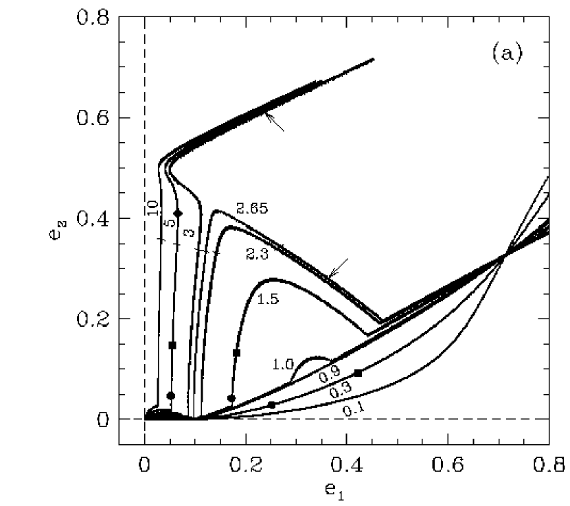
Figure 5: Trajectories of 2:1 resonance configurations from differential migration of planets with constant masses and initially nearly circular orbits. The trajectories are labeled by $m_{1}/m_{2}$. The total planetary mass $(m_{1}+m_{2})/m_{0}=10^{-3}$, and the outer planet is forced to migrate inward with ${\dot{a}}_{2}/a_{2}=-10^{-6}/P_{2}$. (a) The $e_{1}$-$e_{2}$ plane in linear scales. The configurations above the dash for $m_{1}/m_{2}=3$, $5$, and $10$ and the configurations between the two dashes for $m_{1}/m_{2}=2.3$ and $2.65$ have intersecting orbits. The diamond, squares and circles on the curves with $m_{1}/m_{2}=0.3$, $1.5$ and $5$ indicate the equilibrium eccentricities for eccentricity damping of the outer planet with $K=|{\dot{e}}_{2}/e_{2}|/|{\dot{a}}_{2}/a_{2}|=1$, $10$ and $100$, respectively. See text for $K=1$ and $m_{1}/m_{2}=0.3$ and $1.5$. The configurations indicated by the arrows on the curves with $m_{1}/m_{2}=2.65$ and $3$ are used as initial conditions for calculations in §3.2 and Figs. 7 and 8. (b) The small eccentricity region of the $e_{1}$-$e_{2}$ plane in logarithmic scales. The solid lines show the relationship in eq. (7) from the resonant perturbation theory to the lowest order in the eccentricities. The dashed line is the boundary below which the $\theta_{1}=0^{\circ}$ and $\theta_{2}=180^{\circ}$ configuration exists, as determined by Beaugé et al. (2003).

Table 1: Sequences of 2:1 Resonance Configurations from Differential Migration of Planets with Constant Masses

Planetary Mass Ratio		Libration Centers $(\theta_{1},\theta_{2})$
$\phantom{0.95\lesssim}~{}m_{1}/m_{2}\lesssim 0.95$		$(0^{\circ},180^{\circ})\rightarrow(0^{\circ},0^{\circ})$
$0.95\lesssim m_{1}/m_{2}\lesssim 2.55$		$(0^{\circ},180^{\circ})\rightarrow(0^{\circ},0^{\circ})\rightarrow$ asymmetric librations $\rightarrow(0^{\circ},0^{\circ})$
$2.55\lesssim m_{1}/m_{2}\lesssim 2.75$		$(0^{\circ},180^{\circ})\rightarrow$ asymmetric librations $\rightarrow(0^{\circ},0^{\circ})$
$2.75\lesssim m_{1}/m_{2}~{}\phantom{\gtrsim 2.75}$		$(0^{\circ},180^{\circ})\rightarrow$ asymmetric librations

A convenient and informative way to summarize the results for different $m_{1}/m_{2}$ is to plot the trajectories in the $e_{1}$-$e_{2}$ plane (Beaugé et al. 2003; Ferraz-Mello et al. 2003). Figure 5 shows the trajectories for several values of $m_{1}/m_{2}$ between $0.1$ and $10$, with Figure 5a in linear scales and Figure 5b showing the small eccentricity region in logarithmic scales. The trajectories for $m_{1}/m_{2}\lesssim 0.95$, $0.95\lesssim m_{1}/m_{2}\lesssim 2.55$, $2.55\lesssim m_{1}/m_{2}\lesssim 2.75$, and $m_{1}/m_{2}\gtrsim 2.75$ [with the sequences of libration centers $(\theta_{1},\theta_{2})$ summarized in Table 1] are clearly distinguished in the $e_{1}$-$e_{2}$ plane. The transition from $(\theta_{1},\theta_{2})\approx(0^{\circ},180^{\circ})$ at small eccentricities to $(\theta_{1},\theta_{2})\approx(0^{\circ},0^{\circ})$ for $m_{1}/m_{2}\lesssim 2.55$ occurs when $e_{1}\approx 0.1$ and $e_{2}\approx 0$, and the transition to asymmetric librations for $m_{1}/m_{2}\gtrsim 2.55$ occurs before $e_{1}$ reaches $0.1$, with the critical value of $e_{1}$ smaller for larger $m_{1}/m_{2}$ (see Fig. 5b). Beaugé et al. (2003) have determined the boundary in $e_{1}$-$e_{2}$ space below which the $\theta_{1}=0^{\circ}$ and $\theta_{2}=180^{\circ}$ configuration exists, using an analytic model for the resonant Hamiltonian (with an expansion in eccentricities). Their result is well approximated by the relationship $e_{2}=-0.36e_{1}+0.035$, which is shown as the dashed line in Figure 5b. It is in good agreement with the boundary in our numerical results.

For coplanar orbits, the equation for the variation of the periapse longitude is

$${d\varpi_{j}\over dt}=-{\sqrt{1-e_{j}^{2}}\over m_{j}e_{j}\sqrt{Gm_{0}a_{j}}}\,{\partial\Phi\over\partial e_{j}},$$ (5)

where the disturbing potential

$$\Phi=-{Gm_{1}m_{2}\over a_{2}}\varphi(\beta,e_{1},e_{2},\theta_{1},\theta_{2}),$$ (6)

$\varphi$ is a function of the indicated variables, and $\beta=a_{1}/a_{2}\approx 2^{-2/3}$, if we consider only the resonant terms and neglect terms of order $[(m_{1}+m_{2})/m_{0}]^{2}$ and higher (see, e.g., Lee & Peale 2002; Beaugé & Michtchenko 2003). To the lowest order in the eccentricities, $d\varpi_{1}/dt=\beta n_{1}(m_{2}/m_{0})C_{1}/e_{1}$ and $d\varpi_{2}/dt=-n_{2}(m_{1}/m_{0})C_{2}/e_{2}$ for $\theta_{1}=0^{\circ}$ and $\theta_{2}=180^{\circ}$, where $n_{j}$ are the mean motions and $C_{1}(\beta)=-1.19$ and $C_{2}(\beta)=+0.43$ are, respectively, the coefficients of the $e_{1}\cos\theta_{1}$ and $e_{2}\cos\theta_{2}$ terms of the disturbing potential (Lee & Peale, 2002). Thus, for 2:1 resonance configurations with sufficiently small eccentricities, the precessions of the orbits are retrograde, and the requirement that the orbits on average precess at the same rate implies the following relationship between the forced eccentricities:

$$e_{2}/e_{1}=-\beta^{1/2}(C_{2}/C_{1})(m_{1}/m_{2})=0.29(m_{1}/m_{2}).$$ (7)

Our numerical results have finite widths in $e_{1}$ and $e_{2}$ due to finite libration amplitudes, but they are on average in good agreement with equation (7) (solid lines in Fig. 5b) for sufficiently small eccentricities. We terminate the solid lines in Figure 5b at $e_{1}=0.12/(m_{1}/m_{2}+3)$, which is an estimate of where significant deviation from equation (7) would occur, based on the position of the local maximum of $e_{2}$ for $m_{1}/m_{2}\ll 1$ and the boundary in $e_{1}$-$e_{2}$ space for the $\theta_{1}=0^{\circ}$ and $\theta_{2}=180^{\circ}$ configuration.

As we just mentioned, the orbital precessions are retrograde for the resonance configurations with small eccentricities. The precessions remain retrograde throughout the trajectories shown in Figure 5a for $m_{1}/m_{2}\gtrsim 2.75$. On the other hand, all of the trajectories for $m_{1}/m_{2}\lesssim 2.75$ pass through a point with $e_{1}=0.714$ and $e_{2}=0.326$, where $d\varpi_{1}/dt=d\varpi_{2}/dt=0$ and the precessions of the orbits change from retrograde to prograde. (Lee & Peale 2002 have already noted the change from retrograde to prograde precessions for systems with masses like those in GJ 876.) According to equations (5) and (6), the masses only appear as overall factors in $d\varpi_{j}/dt$, with $d\varpi_{1}/dt\propto m_{2}/\sqrt{m_{0}}$ and $d\varpi_{2}/dt\propto m_{1}/\sqrt{m_{0}}$. Thus for small amplitude librations and nearly constant $e_{j}$ and $\theta_{j}$, the combinations of $e_{j}$ and $\theta_{j}$ for which $d\varpi_{1}/dt=d\varpi_{2}/dt$ is nonzero depend only on $m_{1}/m_{2}$, and the combinations for which $d\varpi_{1}/dt=d\varpi_{2}/dt=0$ are independent of the planetary and stellar masses. Since all of the cases in Figure 5a with $m_{1}/m_{2}\lesssim 2.75$ have $\theta_{1}$ and $\theta_{2}$ librating about $0^{\circ}$ at large $e_{1}$, the only point on the $e_{1}$-$e_{2}$ plane where the trajectories can intersect is a combination of $e_{1}$ and $e_{2}$ for which $d\varpi_{1}/dt=d\varpi_{2}/dt=0$.

In our discussion above of the case with $m_{1}/m_{2}=5$, we pointed out that the asymmetric libration configurations with $e_{2}\gtrsim 0.35$ have intersecting orbits (see, e.g., Fig. 2d). Ferraz-Mello et al. (2003) have stated that configurations with the apocentric distance of the inner planet greater than the pericentric distance of the outer planet [i.e., $a_{1}(1+e_{1})>a_{2}(1-e_{2})$ for $m_{1},m_{2}\ll m_{0}$] may have intersecting orbits, but this condition is necessary but not sufficient (it is both necessary and sufficient only for anti-aligned configurations such as those discussed in §4.2). We have determined which of the configurations shown in Figure 5a actually have intersecting orbits. For $m_{1}/m_{2}=3$, $5$, and $10$, the configurations above the dash on each trajectory have intersecting orbits. However, configurations with intersecting orbits are not limited to $m_{1}/m_{2}\gtrsim 2.75$. For $m_{1}/m_{2}=2.3$ and $2.65$, the configurations between the two dashes on each trajectory also have intersecting orbits.

3.2 Effects of Migration Rate, Total Planetary Mass, and Eccentricity Damping

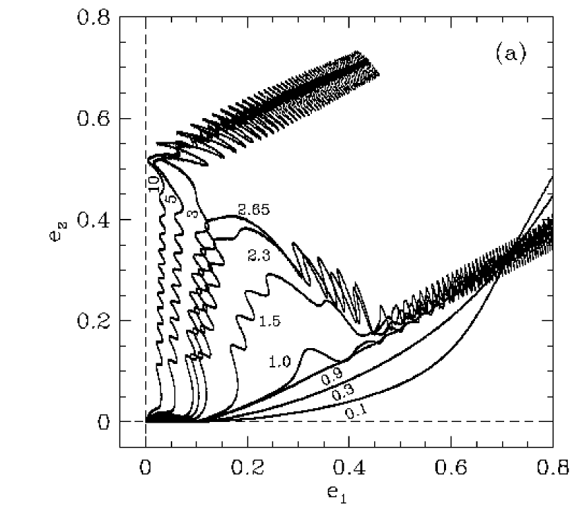
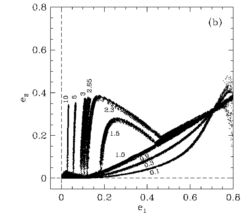
Figure 6: Same as Fig. 5a, but for ${\dot{a}}_{2}/a_{2}=-10^{-4}/P_{2}$ and (a) $(m_{1}+m_{2})/m_{0}=10^{-3}$ and (b) $(m_{1}+m_{2})/m_{0}=10^{-2}$. The basic trajectories depend only on $m_{1}/m_{2}$, but the libration amplitudes and the point at which a sequence becomes unstable can be sensitive to the migration rate and the total planetary mass.

We consider next the effects of a migration rate on the disk viscous timescale similar to that in equation (LABEL:vistime) and a larger total planetary mass. We have performed differential migration calculations similar to those in §3.1, but with ${\dot{a}}_{2}/a_{2}=-10^{-4}/P_{2}$ and $(m_{1}+m_{2})/m_{0}=10^{-3}$ and $10^{-2}$, and the trajectories of stable resonance configurations in the $e_{1}$-$e_{2}$ plane are shown in Figures 6a and 6b, respectively. Figures 5a and 6 show that the basic trajectories depend only on $m_{1}/m_{2}$ and not on the total planetary mass, in agreement with the analysis in §3.1 based on the requirement of equal precession rates. However, the libration amplitudes and the point at which a sequence becomes unstable can be sensitive to the migration rate and the total planetary mass.

For $(m_{1}+m_{2})/m_{0}=10^{-3}$, the faster migration rate (Fig. 6a) leads to larger libration amplitudes when a system with $m_{1}/m_{2}\gtrsim 0.95$ enters asymmetric libration, and the point at which a system with $m_{1}/m_{2}\gtrsim 2.75$ becomes unstable is slightly different from that shown in Figure 5a. All of the trajectories in Figure 6b for $(m_{1}+m_{2})/m_{0}=10^{-2}$ are wider than those in Figure 5a because the larger eccentricity variations generated by the larger total planetary mass before resonance capture lead to resonance configurations with larger libration amplitudes. On the other hand, although the trajectories in Figures 6a and 6b are for the same migration rate, those in Figure 6b with $m_{1}/m_{2}\gtrsim 0.95$ do not show any significant increase in the libration amplitudes when a system enters asymmetric libration, because the larger total planetary mass means that the resonant interaction between the planets is stronger relative to the forced migration. It is not clear in Figure 6b, but with the use of Jacobi coordinates (see §2), we are able to see the capture into the $\theta_{1}\approx 0^{\circ}$ and $\theta_{2}\approx 180^{\circ}$ configuration at small eccentricities when we examine time evolution plots (like those in Figs. 1, 3, and 4) for these calculations with $(m_{1}+m_{2})/m_{0}=10^{-2}$.

In Figure 6b, many of the trajectories for $m_{1}/m_{2}\leq 2.3$ show deviations from the trajectories in Figure 5a at $e_{1}\gtrsim 0.75$ due to rapid increase in the libration amplitudes before the system becomes unstable (see §4.1 for a more detailed discussion of a similar case). The cases with $m_{1}/m_{2}\geq 2.65$ become unstable near the points where the orbits become intersecting (dashes on the trajectories in Fig. 5a). Note, however, that the case with $m_{1}/m_{2}=2.3$ passes through the configurations with intersecting orbits without becoming unstable. The fact that a sequence becomes unstable at a certain point does not mean that all configurations beyond that point are necessarily unstable, especially for smaller libration amplitudes. We have used the asymmetric configuration, with non-intersecting orbits, indicated by the arrow on the curve with $m_{1}/m_{2}=2.65$ in Figure 5a as the starting point for a calculation in which $m_{1}+m_{2}$ is increased from $10^{-3}m_{0}$ at a rate of $d\ln\left(m_{1}+m_{2}\right)/dt=10^{-6}/P_{2,0}$ while $m_{1}/m_{2}$ is kept constant. It remains stable to the end of the calculation when $(m_{1}+m_{2})/m_{0}=10^{-2}$. When we used instead the asymmetric configuration, with intersecting orbits, indicated by the arrow on the curve with $m_{1}/m_{2}=3$ in Figure 5a as the starting point, the configuration becomes unstable when $(m_{1}+m_{2})/m_{0}$ exceeds $0.0033$.

As we mentioned in §1, either eccentricity damping or the termination of migration due to nebula dispersal would lead to a system being left somewhere along a sequence in Figures 5 and 6. There is significant uncertainty in both the sign and the magnitude of the net effect of planet-disk interaction on the orbital eccentricity of the planet because of sensitivity to the distribution of disk material near the locations of the Lindblad and corotation resonances (e.g., Goldreich & Sari 2003). Nevertheless, hydrodynamic simulations of two planets orbiting inside an outer disk have shown eccentricity damping of the outer planet, with $K=|{\dot{e}}_{2}/e_{2}|/|{\dot{a}}_{2}/a_{2}|\sim 1$ (Kley et al., 2004), while an explanation of the observed eccentricities of the GJ 876 system as equilibrium eccentricities requires $K\sim 100$ (Lee & Peale, 2002). To study the effects of eccentricity damping, we have repeated the $m_{1}/m_{2}=0.3$, $1.5$, and $5$ calculations shown in Figures 1, 3, and 4 with $K=1$, $10$, and $100$. For $K=10$ and $100$, the eccentricities reach equilibrium values in all cases, and they are indicated by the squares and circles in Figure 5a. For $K=1$, while the eccentricities in the $m_{1}/m_{2}=5$ calculation reach equilibrium values indicated by the diamond in Figure 5a, those in the $m_{1}/m_{2}=0.3$ and $1.5$ calculations are still increasing at the end of the calculations when $e_{1}\approx 0.68$ and $0.70$, respectively.

4 OTHER RESONANCE CONFIGURATIONS

4.1 Symmetric and Asymmetric Configurations

The bifurcation of the trajectories in Figure 5a at $m_{1}/m_{2}\approx 2.75$ leaves an empty region in the $e_{1}$-$e_{2}$ plane. In this subsection we show that there are stable 2:1 resonance configurations in the empty region of Figure 5a that cannot reached by the scenario considered in §3 (i.e., differential migration of planets with constant masses and initially nearly circular orbits).

Figure 7: Evolution of the eccentricities, $e_{1}$ and $e_{2}$, mean-motion resonance variables, $\theta_{1}$ and $\theta_{2}$, and mass ratio $m_{1}/m_{2}$ for a calculation in which the configuration indicated by the arrow on the curve with $m_{1}/m_{2}=3$ in Fig. 5a is used as the starting point and $m_{1}/m_{2}$ is decreased at a rate of $d\ln(m_{1}/m_{2})/dt=-10^{-6}/P_{2,0}$. The configurations with $m_{1}/m_{2}=1$, $0.3$, and $0.1$ indicated by the dashed lines are used as initial conditions for calculations in Figs. 9 and 11 and §4.3.

Figure 8: Same as Fig. 7, but for a calculation in which the configuration indicated by the arrow on the curve with $m_{1}/m_{2}=2.65$ in Fig. 5a is used as the starting point and $m_{1}/m_{2}$ is increased at a rate of $d\ln(m_{1}/m_{2})/dt=10^{-6}/P_{2,0}$. The configurations with $m_{1}/m_{2}=3$, $5$, and $10$ indicated by the dashed lines are used as initial conditions for calculations in Figs. 10 and 11 and §4.3.

In Figure 7 we show the results of a calculation in which the asymmetric configuration indicated by the arrow on the curve with $m_{1}/m_{2}=3$ in Figure 5a is used as the starting point and $m_{1}/m_{2}$ is decreased from 3 to 0.1 at a rate of $d\ln(m_{1}/m_{2})/dt=-10^{-6}/P_{2,0}$ while $(m_{1}+m_{2})/m_{0}=10^{-3}$ is kept constant. As $m_{1}/m_{2}$ decreases, $\theta_{1}$ and $\theta_{2}$ remain near the initial values, $e_{2}$ changes little, and $e_{1}$ increases (i.e., the sequence extends to the right in the $e_{1}$-$e_{2}$ plane). Similarly, we have used the asymmetric configuration indicated by the arrow on the curve with $m_{1}/m_{2}=2.65$ in Figure 5a as the starting point for a calculation in which $m_{1}/m_{2}$ is increased from 2.65 to 10 at a rate of $d\ln(m_{1}/m_{2})/dt=10^{-6}/P_{2,0}$. The results are shown in Figure 8. As $m_{1}/m_{2}$ increases, $\theta_{1}$ and $\theta_{2}$ remain near the initial values, $e_{1}$ changes little, and $e_{2}$ increases (i.e., the sequence extends upward in the $e_{1}$-$e_{2}$ plane). Thus we have found for each $m_{1}/m_{2}$ between $0.1$ and $10$ a resonance configuration distinct from those shown in Figure 5a.

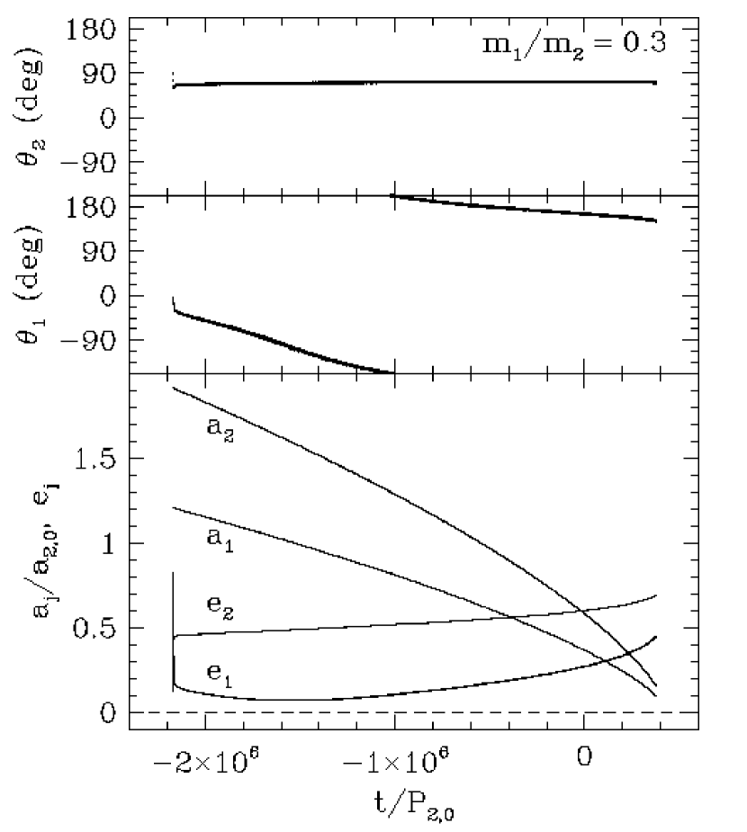
Figure 9: Resonance configurations from forward and backward migration calculations using the $m_{1}/m_{2}=0.3$ configuration from Fig. 7 as initial conditions. The results from the calculations with ${\dot{a}}_{2}/a_{2}=-10^{-6}/P_{2}$ and $10^{-6}/P_{2}$ are plotted along the positive and negative time axis, respectively. These resonance configurations are different from those in Fig. 1 from differential migration of planets with constant masses and initially nearly circular orbits.

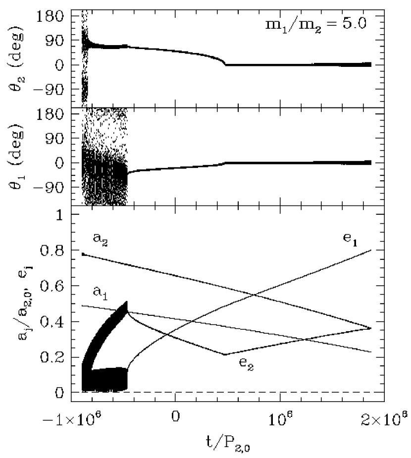
Figure 10: Same as Fig. 9, but for calculations using the $m_{1}/m_{2}=5$ configuration from Fig. 8 as initial conditions. The configurations at $t/P_{2,0}\gtrsim-4.6\times 10^{5}$ with both $\theta_{1}$ and $\theta_{2}$ librating are different from those in Fig. 4.

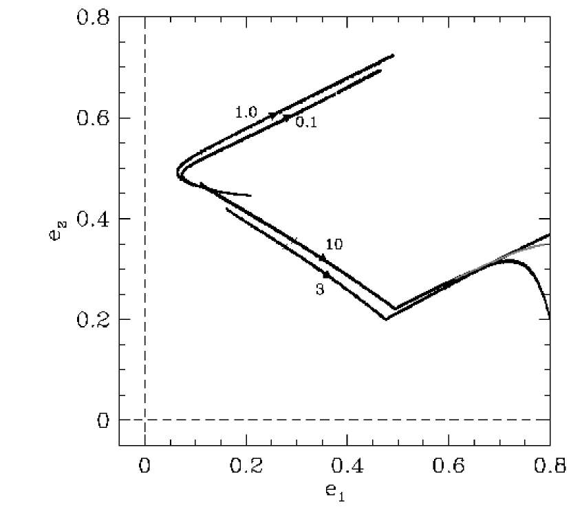
Figure 11: Trajectories in the $e_{1}$-$e_{2}$ plane of 2:1 resonance configurations from forward and backward migration calculations with initial conditions (triangles, oriented to indicate the direction for forward migration) from Figs. 7 and 8 for $m_{1}/m_{2}=0.1$, $1$, $3$, and $10$. See text for the calculation that produces the gray curve for $m_{1}/m_{2}=10$. The resonance configurations are distinct from those in Fig. 5a. All of the configurations for $m_{1}/m_{2}=0.1$ and $1$ and the configurations to the left of the dashes on the trajectories for $m_{1}/m_{2}=3$ and $10$ have intersecting orbits.

For a given $m_{1}/m_{2}$, we can then use the resonance configuration from either Figure 7 (if $m_{1}/m_{2}\lesssim 2.75$) or Figure 8 (if $m_{1}/m_{2}\gtrsim 2.75$) as the starting point for “forward” (${\dot{a}}_{2}/a_{2}<0$) and “backward” (${\dot{a}}_{2}/a_{2}>0$) migration calculations to search for other resonance configurations. Figure 9 shows the results from the $m_{1}/m_{2}=0.3$ calculations with ${\dot{a}}_{2}/a_{2}=-10^{-6}/P_{2}$ and $10^{-6}/P_{2}$ along the positive and negative time axis, respectively. In both calculations we have integrated the system until it becomes unstable. The asymmetric resonance configurations in Figure 9 are clearly different from the symmetric and anti-symmetric configurations in Figure 1. Figure 10 shows the results from the $m_{1}/m_{2}=5$ calculations. The calculation with ${\dot{a}}_{2}/a_{2}=-10^{-6}/P_{2}$ was terminated when $e_{1}$ reaches $0.8$, while the calculation with ${\dot{a}}_{2}/a_{2}=10^{-6}/P_{2}$ was terminated when both $\theta_{1}$ and $\theta_{2}$ circulate. We shall not consider further configurations with only $\theta_{2}$ librating, but it is interesting that those in Figure 10 at $-8.5\times 10^{5}\lesssim t/P_{2,0}\lesssim-4.6\times 10^{5}$ are similar to those in Figure 4 at $t/P_{2,0}\lesssim 6\times 10^{5}$ with both $\theta_{1}$ and $\theta_{2}$ librating. The configurations in Figure 10 with both $\theta_{1}$ and $\theta_{2}$ librating (at $t/P_{2,0}\gtrsim-4.6\times 10^{5}$) are either symmetric or asymmetric, and they are clearly different from those in Figure 4.

In Figure 11 we show the trajectories in the $e_{1}$-$e_{2}$ plane of stable resonance configurations (with both $\theta_{1}$ and $\theta_{2}$ librating) from the forward and backward differential migration calculations with initial conditions (triangles in Fig. 11) from Figures 7 and 8 for $m_{1}/m_{2}=0.1$, $1$, $3$, and $10$. The trajectories for $m_{1}/m_{2}=0.3$ and $5$, whose time evolutions are shown in Figures 9 and 10, respectively, are simply between the appropriate pairs in Figure 11 and are not shown to avoid crowding. Unlike the cases with $m_{1}/m_{2}=3$ and $5$ (see Fig. 10 for the latter), where $e_{2}$ increases monotonically with increasing $e_{1}$ for the $\theta_{1}\approx\theta_{2}\approx 0^{\circ}$ configurations at large $e_{1}$, the trajectory for $m_{1}/m_{2}=10$ shows a maximum in $e_{2}$ at $e_{1}\approx 0.72$. This turns out to be due to the libration amplitudes of $\theta_{1}$ and $\theta_{2}$ becoming too large. As the example in Figure 10 shows, the libration amplitudes of $\theta_{1}$ and $\theta_{2}$ increase as the system is driven deeper into resonance. The semi-amplitudes do not exceed $10^{\circ}$ in the cases with $m_{1}/m_{2}=3$ and $5$, but for $m_{1}/m_{2}=10$, the configurations with $e_{1}\gtrsim 0.68$ have semi-amplitudes of $\theta_{1}$ and $\theta_{2}>10^{\circ}$ (although $\theta_{1}$ and $\theta_{2}$ are nearly in phase so that the libration amplitude of $\theta_{3}=\theta_{1}-\theta_{2}$ remains small and the trajectory in the $e_{1}$-$e_{2}$ plane remains narrow). We have repeated the $m_{1}/m_{2}=10$ calculation by starting at $e_{1}=0.61$ with initial conditions that correspond to smaller libration amplitudes. The resulting trajectory is shown as the gray curve in Figure 11, and it does not show the decrease in $e_{2}$ at large $e_{1}$.

Like the trajectories in Figure 5a for $m_{1}/m_{2}\lesssim 2.75$, the trajectories in Figure 11 for $m_{1}/m_{2}=3$ and $10$ (the gray curve for the latter) also pass through the point with $e_{1}=0.714$ and $e_{2}=0.326$, where $d\varpi_{1}/dt=d\varpi_{2}/dt=0$ and the precessions of the orbits change from retrograde at smaller $e_{1}$ to prograde at larger $e_{1}$. In Figure 11, all of the configurations for $m_{1}/m_{2}=0.1$ and $1$ and the configurations to the left of the dashes on the trajectories for $m_{1}/m_{2}=3$ and $10$ have intersecting orbits.

The configurations shown in Figure 11 clearly occupy a different part of the $e_{1}$-$e_{2}$ plane compared to those in Figure 5a. They are found by a combination of calculations in which $m_{1}/m_{2}$ is changed slowly and differential migration calculations, and cannot be reached by differential migration of planets with constant masses and initially nearly circular orbits.

4.2 Anti-symmetric Configurations with $\theta_{1}\approx 180^{\circ}$ and $\theta_{2}\approx 0^{\circ}$

Figure 12: Anti-symmetric resonance configuration with $\theta_{1}\approx 180^{\circ}$, $\theta_{2}\approx 0^{\circ}$, and intersecting orbits used as the starting point for calculations in Fig. 13.

Figure 13: Evolution of the eccentricities, $e_{1}$ and $e_{2}$, mean-motion resonance variables, $\theta_{1}$ and $\theta_{2}$, and mass ratio $m_{1}/m_{2}$ for calculations in which the configuration shown in Fig. 12 is used as the starting point and $m_{1}/m_{2}$ is increased to $10$ and decreased to $0.1$. The results from the calculations with $d\ln(m_{1}/m_{2})/dt=10^{-6}/P_{2,0}$ and $-10^{-6}/P_{2,0}$ are plotted along the positive and negative time axis, respectively. The configurations with $m_{1}/m_{2}=0.1$, $1$, and $10$ indicated by the dashed lines are used as initial conditions for calculations in Fig. 14.

As we mentioned in §1, Ji et al. (2003) and Hadjidemetriou & Psychoyos (2003) have discovered stable 2:1 resonance configurations with $\theta_{1}\approx 180^{\circ}$ and $\theta_{2}\approx 0^{\circ}$ for systems with masses similar to those of the HD 82943 system announced initially by the Geneva group [$m_{1}/m_{2}=0.54$, $(m_{1}+m_{2})/m_{0}=2.3\times 10^{-3}$]. We have derived from the results of Ji et al. (2003) a $\theta_{1}\approx 180^{\circ}$ and $\theta_{2}\approx 0^{\circ}$ configuration with $m_{1}/m_{2}=0.54$, $(m_{1}+m_{2})/m_{0}=10^{-3}$, and small libration amplitudes, and it is shown in Figure 12. The $\theta_{1}\approx 180^{\circ}$ and $\theta_{2}\approx 0^{\circ}$ configuration has intersecting orbits, with the periapses nearly anti-aligned and conjunctions occurring when the inner planet is near apoapse and the outer planet is near periapse (and closer to the star than the inner planet).

Figure 14: Trajectories in the $e_{1}$-$e_{2}$ plane of 2:1 resonance configurations with $\theta_{1}\approx 180^{\circ}$ and $\theta_{2}\approx 0^{\circ}$ from forward and backward migration calculations with initial conditions (triangles, oriented to indicate the direction for forward migration) from Fig. 13 for $m_{1}/m_{2}=0.1$, $1$, and $10$. These resonance configurations are distinct from those in Figs. 5a and 11. The trajectories terminate above the dashed line, where $a_{1}(1+e_{1})=a_{2}(1-e_{2})$ and the planets would collide at conjunction.

We have used the configuration in Figure 12 as the starting point for calculations in which $m_{1}/m_{2}$ is increased to $10$ and decreased to $0.1$. The results are shown in Figure 13, with the calculations with $d\ln(m_{1}/m_{2})/dt=10^{-6}/P_{2,0}$ and $-10^{-6}/P_{2,0}$ along the positive and negative time axis, respectively. The libration centers remain at $\theta_{1}=180^{\circ}$ and $\theta_{2}=0^{\circ}$, and $e_{1}$ decreases ($e_{2}$ increases) with increasing $m_{1}/m_{2}$. We have thus found for each $m_{1}/m_{2}$ in the range $0.1\leq m_{1}/m_{2}\leq 10$ a resonance configuration with $\theta_{1}\approx 180^{\circ}$ and $\theta_{2}\approx 0^{\circ}$. As in §4.1, we can then use the resonance configuration for a given $m_{1}/m_{2}$ from Figure 13 as the starting point for forward and backward migration calculations to search for other resonance configurations with the same $m_{1}/m_{2}$. Figure 14 shows the trajectories in the $e_{1}$-$e_{2}$ plane of stable resonance configurations from the migration calculations with $m_{1}/m_{2}=0.1$, $1$, and $10$. The initial conditions (triangles in Fig. 14) are indicated by the dashed lines in Figure 13. The calculations with ${\dot{a}}_{2}/a_{2}=-10^{-6}/P_{2}$ were terminated when $e_{2}$ reaches $0.7$, while the calculations with ${\dot{a}}_{2}/a_{2}=10^{-6}/P_{2}$ were terminated when the system becomes unstable. All of the configurations shown in Figure 14 have libration centers at $\theta_{1}=180^{\circ}$ and $\theta_{2}=0^{\circ}$ and retrograde orbital precessions. Along the sequence for a given $m_{1}/m_{2}$, the fractional distance between the planets at conjunction, $(a_{1}/a_{2})(1+e_{1})-(1-e_{2})$, decreases with decreasing $e_{2}$, and the system becomes unstable at a point above the dashed line in Figure 14, where $a_{1}(1+e_{1})=a_{2}(1-e_{2})$ and the planets would collide at conjunction. We can see from Figure 14 that the configurations with $\theta_{1}\approx 180^{\circ}$ and $\theta_{2}\approx 0^{\circ}$ tend to a sequence with $e_{1}=0$ and $e_{2}$ above $0.37$ in the limit $m_{1}/m_{2}\to\infty$. These are the pericentric libration configurations found by Beaugé (1994) for the exterior 2:1 resonance in the planar, circular, restricted three-body problem.

4.3 Effects of Total Planetary Mass

We consider in this subsection the effects of a larger total planetary mass on the stability of the resonance configurations found in §4.1 and §4.2 for $(m_{1}+m_{2})/m_{0}=10^{-3}$. We have used the configurations indicated by the dashed lines in Figure 7 as initial conditions for calculations in which $m_{1}+m_{2}$ is increased at a rate of $d\ln\left(m_{1}+m_{2}\right)/dt=10^{-6}/P_{2,0}$ while $m_{1}/m_{2}$ is kept constant. These configurations with $m_{1}/m_{2}=1$, $0.3$, and $0.1$ become unstable when $(m_{1}+m_{2})/m_{0}$ exceeds $0.0037$, $0.0041$, and $0.0043$, respectively. Similar calculations with the configurations indicated by the dashed lines in Figure 8 with $m_{1}/m_{2}=3$, $5$, and $10$ as initial conditions show that these configurations are stable for $(m_{1}+m_{2})/m_{0}$ up to at least $10^{-2}$.

For the anti-symmetric configurations with $\theta_{1}\approx 180^{\circ}$ and $\theta_{2}\approx 0^{\circ}$, the minimum $e_{2}$ (and the minimum fractional distance between the planets at conjunction) at which the configurations become unstable increases with increasing total planetary mass. We have used the configurations at the top of the trajectories shown in Figure 14 with $e_{2}\approx 0.7$ and $m_{1}/m_{2}=0.1$, $1$, and $10$ as initial conditions for calculations in which $m_{1}+m_{2}$ is increased, and they remain stable to the end of the calculations when $(m_{1}+m_{2})/m_{0}=10^{-2}$. When we used instead the configurations indicated by the triangles in Figure 14 as initial conditions, the cases with $m_{1}/m_{2}=0.1$ and $1$ are stable for $(m_{1}+m_{2})/m_{0}$ up to at least $10^{-2}$, but the case with $m_{1}/m_{2}=10$ becomes unstable when $(m_{1}+m_{2})/m_{0}$ exceeds $0.0096$.

It is likely that many (if not all) of the asymmetric configurations shown in Figure 9 for $m_{1}/m_{2}=0.3$ (which is close to $m_{1}/m_{2}=0.32$ of the GJ 876 planets) are unstable for the total mass of the GJ 876 planets [$(m_{1}+m_{2})/m_{0}=0.0095$], because the configuration at $t=0$ is the $m_{1}/m_{2}=0.3$ configuration from Figure 7 examined above and it is unstable for $(m_{1}+m_{2})/m_{0}>0.0041$. Thus for a system with masses like those in GJ 876, there are stable 2:1 resonance configurations with $(\theta_{1},\theta_{2})\approx(180^{\circ},0^{\circ})$, in addition to those with $(\theta_{1},\theta_{2})\approx(0^{\circ},180^{\circ})$ and $(0^{\circ},0^{\circ})$ that can be obtained from differential migration of planets with constant masses. However, the planets are sufficiently massive that asymmetric configurations like those in Figure 9 are probably unstable.

5 DISCUSSION AND CONCLUSIONS

We have shown that there is a diversity of 2:1 resonance configurations for planar two-planet systems. We began with a series of differential migration calculations, with planets having constant masses and initially circular orbits, and found the following types of stable 2:1 resonance configurations: (1) anti-symmetric configurations with the mean-motion resonance variables $\theta_{1}=\lambda_{1}-2\lambda_{2}+\varpi_{1}$ and $\theta_{2}=\lambda_{1}-2\lambda_{2}+\varpi_{2}$ librating about $0^{\circ}$ and $180^{\circ}$, respectively (as in the Io-Europa pair); (2) symmetric configurations with both $\theta_{1}$ and $\theta_{2}$ librating about $0^{\circ}$ (as in the GJ 876 system); and (3) asymmetric configurations with $\theta_{1}$ and $\theta_{2}$ librating about angles far from either $0^{\circ}$ or $180^{\circ}$. Systems with $m_{1}/m_{2}\lesssim 0.95$, $0.95\lesssim m_{1}/m_{2}\lesssim 2.55$, $2.55\lesssim m_{1}/m_{2}\lesssim 2.75$, and $m_{1}/m_{2}\gtrsim 2.75$ show different types of evolution (Table 1), and their trajectories in the $e_{1}$-$e_{2}$ plane are clearly distinguished (Fig. 5). The basic trajectories depend only on $m_{1}/m_{2}$, but the libration amplitudes and the point at which a sequence becomes unstable can be sensitive to the migration rate and the total planetary mass. Where a system is left along a sequence depends on the magnitude of the eccentricity damping or the timing of the termination of migration due to nebula dispersal. There are also stable 2:1 resonance configurations with symmetric ($\theta_{1}\approx\theta_{2}\approx 0^{\circ}$), asymmetric, and anti-symmetric ($\theta_{1}\approx 180^{\circ}$ and $\theta_{2}\approx 0^{\circ}$) librations that cannot be reached by differential migration of planets with constant masses and initially nearly circular orbits. We have analyzed the properties of the resonance configurations found in our study. The asymmetric configurations with large $e_{2}$ and the $\theta_{1}\approx 180^{\circ}$ and $\theta_{2}\approx 0^{\circ}$ configurations have intersecting orbits, while the $\theta_{1}\approx\theta_{2}\approx 0^{\circ}$ configurations with $e_{1}>0.714$ have prograde orbital precessions. Figures 5, 11, and 14 can be used to determine whether an observed system could be near a 2:1 resonance configuration with both $\theta_{1}$ and $\theta_{2}$ librating.

We now describe several mechanisms by which the resonance configurations summarized in Figures 11 and 14 can be reached. Since we found the symmetric and asymmetric configurations in §4.1 (Fig. 11) by a combination of calculations in which $m_{1}/m_{2}$ is changed and differential migration calculations, they can be reached by differential migration if the planets continue to grow at different rates and $m_{1}/m_{2}$ changes during migration. In particular, if $m_{1}/m_{2}\lesssim 2.75$ when the system is first captured into resonance and $m_{1}/m_{2}$ increases above $2.75$ when $e_{1}\gtrsim 0.17$, the system should cross over to the configurations with $m_{1}/m_{2}\gtrsim 2.75$ in Figure 11. Similarly, if $m_{1}/m_{2}\gtrsim 2.75$ when the system is first captured into resonance and $m_{1}/m_{2}$ decreases below $2.75$ when $e_{2}\gtrsim 0.49$, the system should cross over to the configurations with $m_{1}/m_{2}\lesssim 2.75$ in Figure 11. After the planets open gaps about their orbits and clear the disk material between them, they can continue to grow by accreting gas flowing across their orbits from the inner and outer disks. If the inner disk is depleted, the situation with the outer planet growing faster and a decreasing $m_{1}/m_{2}$ may be more likely (Kley, 2000).

A mechanism by which the $\theta_{1}\approx 180^{\circ}$ and $\theta_{2}\approx 0^{\circ}$ configuration in §4.2 (Fig. 14) can be reached is a migration scenario involving inclination resonances. Thommes & Lissauer (2003) have studied the capture into and evolution in 2:1 resonances due to differential migration for orbits with small initial inclinations. For the case with $m_{1}/m_{2}=1$, the system is initially captured into eccentricity-type mean-motion resonances only (with both $\theta_{1}$ and $\theta_{2}$ librating), and the initial evolution after capture is similar to that of the planar system discussed in §3. But when $e_{1}$ grows to $\sim 0.6$, the system also enters into inclination-type mean-motion resonances (with both $2\lambda_{1}-4\lambda_{2}+2\Omega_{1}$ and $2\lambda_{1}-4\lambda_{2}+2\Omega_{2}$ librating, where $\Omega_{1,2}$ are the longitudes of ascending node), and the orbital inclinations begin to grow. The system eventually evolves out of the inclination resonances, and interestingly, the eccentricity resonances switch from the $\theta_{1}\approx\theta_{2}\approx 0^{\circ}$ configuration to the $\theta_{1}\approx 180^{\circ}$ and $\theta_{2}\approx 0^{\circ}$ configuration at the same time. Thommes & Lissauer (2003) have noted that the inclination resonances are not encountered until $e_{1}$ grows to $\sim 0.6$, which requires $m_{1}/m_{2}$ to be less than about $2$ for planets with constant masses. From the results in §3 (Fig. 5a), we find that the boundary in $m_{1}/m_{2}$ for $e_{1}$ to reach $\sim 0.6$ is more precisely $m_{1}/m_{2}\lesssim 2.75$. However, if we allow $m_{1}/m_{2}$ to change during migration as described in the previous paragraph, it would be possible for $e_{1}$ to grow to $\sim 0.6$ even for systems with final $m_{1}/m_{2}\gtrsim 2.75$ (see Fig. 11). Thus it may be possible to reach the $\theta_{1}\approx 180^{\circ}$ and $\theta_{2}\approx 0^{\circ}$ configuration by evolving through inclination resonances for non-coplanar systems with a wide range of final $m_{1}/m_{2}$.

Finally, there is a mechanism for establishing mean-motion resonances in planetary systems that does not involve migration due to planet-disk interaction. Levison, Lissauer, & Duncan (1998) have found that a significant fraction of systems at the end of a series of simulations starting with a large number of planetary embryos has mean-motion resonances. More recently, Adams & Laughlin (2003) have performed a series of $N$-body simulations of crowded planetary systems, with $10$ giant planets initially in the radial range $5{\rm\,AU}\leq a\leq 30{\rm\,AU}$. After $10^{6}{\rm\,yr}$, there are often only two or three planets remaining in a system, and a surprisingly large fraction ($\sim 10\%$) of the systems have a pair of planets near resonance (roughly equally distributed among the 2:1, 3:2, and 1:1 resonances), although not all of the resonant pairs will survive on longer timescales. If there is no additional damping mechanism, the resonance configurations produced by multiple-planet scattering in crowded planetary systems are likely to have moderate to large orbital eccentricities and relatively large libration amplitudes. A more detailed analysis of the resonances produced by this mechanism is needed, but there is no obvious reason to suspect that it cannot produce any of the 2:1 resonance configurations with moderate to large orbital eccentricities presented in §3 and §4, provided that the configuration is stable for relatively large libration amplitudes.

The number of multiple-planet systems is expected to increase significantly in the next few years. Our results show that a wide variety of 2:1 resonance configurations can be expected among future discoveries and that their geometry can provide information about the origin of the resonances.

References

- Adams & Laughlin (2003) Adams, F. C., & Laughlin, G. 2003, Icarus, 163, 290
- Beaugé (1994) Beaugé, C. 1994, Celest. Mech. Dyn. Astron., 60, 225
- Beaugé et al. (2003) Beaugé, C., Ferraz-Mello, S., & Michtchenko, T. A. 2003, ApJ, 593, 1124
- Beaugé & Michtchenko (2003) Beaugé, C., & Michtchenko, T. A. 2003, MNRAS, 341, 760
- Bryden et al. (2000) Bryden, G., Różyczka, M., Lin, D. N. C., & Bodenheimer, P. 2000, ApJ, 540, 1091
- Duncan et al. (1998) Duncan, M. J., Levison, H. F., & Lee, M. H. 1998, AJ, 116, 2067
- Ferraz-Mello et al. (2003) Ferraz-Mello, S., Beaugé, C., & Michtchenko, T. A. 2003, Celest. Mech. Dyn. Astron., 87, 99
- Goldreich & Sari (2003) Goldreich, P., & Sari, R. 2003, ApJ, 585, 1024
- Hadjidemetriou & Psychoyos (2003) Hadjidemetriou, J. D., & Psychoyos, D. 2003, in Galaxies and Chaos, ed. G. Contopoulos & N. Voglis (Berlin: Springer), 412
- Ji et al. (2003) Ji, J., Kinoshita, H., Liu, L., Li, G., & Nakai, H. 2003, Celest. Mech. Dyn. Astron., 87, 113
- Kley (2000) Kley, W. 2000, MNRAS, 313, L47
- Kley et al. (2004) Kley, W., Peitz, J., & Bryden, G. 2004, A&A, 414, 735
- Laughlin & Chambers (2001) Laughlin, G., & Chambers, J. E. 2001, ApJ, 551, L109
- Lee & Peale (2002) Lee, M. H., & Peale, S. J. 2002, ApJ, 567, 596
- Lee & Peale (2003a) Lee, M. H., & Peale, S. J. 2003a, in Scientific Frontiers in Research on Extrasolar Planets, ed. D. Deming & S. Seager (San Francisco: ASP), 197
- Lee & Peale (2003b) Lee, M. H., & Peale, S. J. 2003b, ApJ, 592, 1201
- Levison et al. (1998) Levison, H. F., Lissauer, J. J., & Duncan, M. J. 1998, AJ, 116, 1998
- Malhotra (1999) Malhotra, R. 1999, Lunar Planet. Sci., XXX, 1998
- Marcy et al. (2002) Marcy, G. W., Butler, R. P., Fischer, D. A., Laughlin, G., Vogt, S. S., Henry, G. W., & Pourbaix, D. 2002, ApJ, 581, 1375
- Marcy et al. (2001) Marcy, G. W., Butler, R. P., Fischer, D., Vogt, S. S., Lissauer, J. J., & Rivera, E. J. 2001, ApJ, 556, 296
- Mayor et al. (2004) Mayor, M., Udry, S., Neaf, D., Pepe, F., Queloz, D., Santos, N. C., & Burnet, M. 2004, A&A, 415, 391
- Message (1958) Message, P. J. 1958, AJ, 63, 443
- Rivera & Lissauer (2001) Rivera, E. J., & Lissauer, J. J. 2001, ApJ, 558, 392
- Snellgrove et al. (2001) Snellgrove, M. D., Papaloizou, J. C. B., & Nelson, R. P. 2001, A&A, 374, 1092
- Thommes & Lissauer (2003) Thommes, E. W., & Lissauer, J. J. 2003, ApJ, 597, 566
- Ward (1997) Ward, W. R. 1997, Icarus, 126, 261
- Wisdom & Holman (1991) Wisdom, J., & Holman, M. 1991, AJ, 102, 1528