The X-ray and radio emission from SN 2002ap:
The importance of Compton scattering

Abstract

The radio and X-ray observations of the Type Ic supernova SN 2002ap are modeled. We find that inverse Compton cooling by photospheric photons explains the observed steep radio spectrum, and also the X-ray flux observed by XMM. Thermal emission from the shock is insufficient to explain the X-ray flux. The radio emitting region expands with a velocity of $\sim 70,000\rm~{}km~{}s^{-1}$. From the ratio of X-ray to radio emission we find that the energy densities of magnetic fields and relativistic electrons are close to equipartion. The mass loss rate of the progenitor star depends on the absolute value of $\epsilon_{\rm B}$, and is given by $\dot{M}\approx 1\times 10^{-8}(v_{\rm w}/1000\rm~{}km~{}s^{-1})\epsilon_{\rm B}^{-1}~{}M_{\odot}~{}\rm yr^{-1}$.

1 Introduction

The connection between Type Ic supernovae (SNe) and gamma-ray bursts (GRBs), as recently highlighted by GRB030329=SN2003dh (Stanek et al., 2003; Hjorth et al., 2003; Kawabata et al., 2003), have made a detailed understanding of this class of SNe especially urgent. The first indication of an association of GRBs with Type Ic SNe was, however, already clear from the observations of GRB980425=SN1998bw (e.g., Iwamoto et al., 2003). Type Ic SNe are believed to be the result of explosions of Wolf-Rayet stars, which have lost their hydrogen and most of their helium envelopes (Nomoto et al., 1994; Woosley, Langer, & Weaver, 1995). Progenitors of this type have strong stellar winds with mass loss rates $\dot{M}\sim 10^{-5}~{}M_{\odot}~{}\rm yr^{-1}$ and wind velocities $v_{\rm w}\sim 1000-4000\rm~{}km~{}s^{-1}$. The interaction of the non-relativistic supernova ejecta with this wind has long been invoked to explain the radio and X-ray emission observed for this type of SNe (e.g., Chevalier & Fransson, 2003). For the GRBs a relativistic version of the same scenario has been used to explain the properties of the GRB afterglows (e.g., Li & Chevalier, 2003).

Because of its small distance, 7.3 Mpc, SN 2002ap has been subject to observations in several wavelength bands from radio to X-rays. The optical spectrum showed the SN to be a typical Type Ic, with no evidence for hydrogen or helium. Although line blending made it hard to determine velocities accurately, Mazzali et al. (2002) argued that SN 2002ap belongs to the extremely energetic events sometimes referred to as ’hypernovae’, where the prime example is SN 1998bw. The total kinetic energy is, however, sensitive to the fraction of the ejecta at very high velocity, which is not probed by the optical spectra. Radio and X-ray observations are more sensitive to this part of the ejecta, since radiation in these wavelength bands are expected to arise in the shocked, faster moving outer material. Hence, an accurate modeling of the radio and X-ray observations is well motivated.

Radio observations of SN 2002ap with VLA, and modeling of these, have been discussed in Berger, Kulkarni, & Chevalier (2002) (in the following BKC). With the assumption of equipartion between magnetic fields and relativistic electrons, these authors showed that the radio light curves could be explained by a synchrotron self-absorption model, where the radio emitting material expands at $\sim 0.3$ c. While the fits to the light curves were satisfactory, there are some issues left open by the model. In particular, the implied optical thin synchrotron spectrum is considerably flatter than the observed one. The steeper than expected spectrum could be due to synchrotron cooling. If so, a magnetic field strength much in excess of equipartion is required.

In parallel to this, there has been several papers discussing XMM observations of SN 2002ap (Soria & Kong, 2002; Sutaria, Chandra, Bhatnagar, & Ray, 2003; Soria, Pian, & Mazzali, 2004). These authors have interpreted the X-ray emission as coming from the thermal electrons behind the shock either directly as free-free emission or as inverse Compton scattering of the photospheric SN photons. For such models to work, the shock velocity has to be fairly low ($\sim 10,000-20,000\rm~{}km~{}s^{-1}$ at day 6). As we argue in this paper, there is evience from optical line profiles that velocities higher than this are needed. Furthermore, a low shock velocity implies a small size of the radio emission region and, hence, a high brightness temperature.

In this paper we show that a consistent picture of both the radio and X-ray observations can be obtained by a model where inverse Compton cooling of the relativistic electrons by the photospheric photons is important. This explains both the steep radio spectrum, and the X-ray emission as coming from the same region, expanding at a velocity compatible with both optical and radio observations. The inclusion of the X-ray constraint also allows a determination of the ratio between the energy densities in magnetic fields and relativistic electrons.

The paper is organized as follows. In §2 we discuss the constraints on different cooling processes of the relativistic electrons, using simple analytical arguments. In §3 we illustrate this by a detailed model calculation of the observed light curves and radio and X-ray spectra. The implications of this and a comparison with related papers are given in §4. In §5 we summarize our conclusions. We will in the following use a distance of $D\approx 7.3$ Mpc for M 74 (Sharina, Karachentsev, & Tikhonov, 1996).

2 Analytical considerations.

An approximate expression for the optically thin synchrotron luminosity, $L_{\nu}$, emitted at a frequency $\nu$ from behind a spherically symmetric, non-relativistic shock with velocity $v_{\rm sh}$ and radius $R_{\rm sh}$ is given by

$$\nu L_{\nu}\approx\pi R_{\rm sh}^{2}v_{\rm sh}n_{\rm rel}\left(\frac{\gamma_{\nu}}{\gamma_{\rm min}}\right)^{1-p}\gamma_{\nu}mc^{2}\left(1+\frac{t_{\rm synch}(\nu)}{t}+\frac{t_{\rm synch}(\nu)}{t_{\rm other}(\nu)}\right)^{-1}.$$ (1)

(e.g., Fransson & Björnsson, 1998). The number density of relativistic electrons is denoted by $n_{\rm rel}$ and $\gamma_{\nu}$ is the Lorentz factor of electrons radiating at a typical frequency $\nu\propto\gamma_{\nu}^{2}B$, where $B$ is the strength of the magnetic field. The energy distribution of the relativistic electrons injected behind the shock is parameterized as $dn_{\rm rel}(\gamma)/d\gamma\propto\gamma^{-p}$ for $\gamma_{\rm min}\leq\gamma\leq\gamma_{\rm max}$ and zero otherwise. The second bracket on the RHS of equation (1) is the fraction of the injected energy which is radiated away as synchrotron radiation. This is determined by three different time scales: $t$ is the dynamical time (i.e., the adiabatic cooling time; roughly, the time since the onset of expansion), $t_{\rm synch}(\nu)$ is the synchrotron cooling time for electrons radiating at a frequency $\nu$, and $t_{\rm other}(\nu)$ is the cooling time corresponding to processes other than synchrotron radiation.

The extensive observations of SN 1993J allowed a detailed modeling of the synchrotron radiation produced by the shock. It was shown in Fransson & Björnsson (1998) that behind the shock, the energy densities of relativistic electrons and magnetic field both scaled with the thermal energy density. Furthermore, the shock expanded into a circumstellar medium in which density ($n_{\rm csm}$) varied with radius as $R^{-2}$. As a result, $n_{\rm rel}\propto B^{2}\propto n_{\rm csm}v_{\rm sh}^{2}\propto t^{-2}$. Implicit in these scaling relations is the assumption of no time variation in $\gamma_{\rm min}$. However, since the deduced value of $p$ was close to two, any variation in $\gamma_{\rm min}$ (and/or $\gamma_{\rm max}$) would only introduce a logarithmic correction. The radio observations of SN 2002ap are such that a detailed modeling is not possible. Hence, in order to limit the scope of our discussion, it will be assumed that the scaling relations obtained for SN 1993J are applicable also for SN 2002ap. This is not a critical assumption; for example, as is shown below, the different scaling relations used by BKC give much the same results. With this background we will now discuss two alternative scenarios, where synchrotron respectively inverse Compton cooling are responsible for the steep radio spectrum.

2.1 Synchrotron radiation as the dominant cooling process

Consider first the case when synchrotron radiation dominates other cooling processes (i.e., $t_{\rm synch}<t_{\rm other}$). With the use of $R_{\rm sh}\approx v_{\rm sh}t$, one obtains from equation (1) the time variation of the optically thin synchrotron luminosity

$$L_{\nu}\propto v_{\rm sh}^{3}\gamma_{\nu}^{2-p}\left(1+\frac{t_{\rm synch}}{t}\right)^{-1}.$$ (2)

When radiative cooling is not important (i.e., $t<t_{\rm synch}$), this leads to

$$L_{\nu} \propto v_{\rm sh}^{3}B^{(p+1)/2}t$$ (3)

$$\propto v_{\rm sh}^{3}t^{(1-p)/2},$$

where $t_{\rm synch}\propto B^{-3/2}$ has been used. When synchrotron cooling is important (i.e., $t>t_{\rm synch}$), the corresponding expression for the synchrotron luminosity is

$$L_{\nu} \propto v_{\rm sh}^{3}B^{(p-2)/2}$$ (4)

$$\propto v_{\rm sh}^{3}t^{(2-p)/2}.$$

The time dependence of $v_{\rm sh}$ in SN 2002ap used by BKC is the one for an ejecta whose structure is thought appropriate for a Ic SN, expanding into a $n_{\rm csm}\propto R^{-2}$ circumstellar medium. The self-similar solution (Chevalier, 1982) then gives $v_{\rm sh}\propto t^{-1/(n-2)}$, where $n$ is the effective power law index of the ejecta density. For the high velocities relevant for SN 2002ap, Matzner & McKee (1999) find $n=10.18$ or $v_{\rm sh}\propto t^{-0.12}$. The observed optically thin synchrotron flux from SN 2002ap varies, roughly, as $F_{\nu}\propto t^{-0.8}$ (BKC). It is seen from equation (3) that this time dependence can be obtained for $v_{\rm sh}\propto t^{-0.12}$ and $p\approx 2$. This is the same conclusion as that reached by BKC, although they used somewhat different scaling relations for the energy densities behind the shock. It is also consistent with an equipartition value for the magnetic field, since such a value implies $t<t_{\rm synch}$. The latter is a necessary requirement for the validity of equation (3). However, this solution predicts an optically thin spectral index $\beta\approx 0.5$, where $L_{\nu}\propto\nu^{-\beta}$. This is not consistent with the observed value $\beta\approx 0.9$. This discrepancy is exacerbated by the fact that the spectral range used to determine $\beta$ is rather close to where optical depth effects become important. Hence, spectral curvature could make the actual spectral index of the optically thin radiation somewhat larger than the measured value of $\beta$.

Short term variations are apparent in the radio light curves. As suggested by BKC, this is likely due to interstellar scattering and scintillation. These variations cause substantial variations in the instantaneous spectral index, which indicates that they are not broad-band. Therefore, a spectral index measured at a given time should be treated with some care. The typical time scale for such flux variations is at most a few hours; hence, the ratio of the fluxes at 4.86 GHz and 8.46 GHz averaged over several days should give a good estimate of the intrinsic optically thin spectral index of SN 2002ap. The value quoted above for the spectral index (i.e., $\beta\approx 0.9$) was obtained by averaging over several observing periods and should thus be robust.

An alternative solution would be to assume $t>t_{\rm synch}$ (i.e., synchrotron cooling is important) and $p\approx 2$, since this gives a value of $\beta$ consistent with the observed one. The luminosity is then obtained from equation (4) as $L_{\nu}\propto v_{\rm sh}^{3}$, which implies $v_{\rm sh}\propto t^{-0.27}$, or $n\approx 6$. Incidentally, this is the same time dependence of the velocity as determined for the type IIb SN 1993J. However, this scenario has a few not so attractive implications, as can be seen from the following arguments.

The thermal energy density ($U_{\rm th}$) behind a non-relativistic supernova shock wave expanding into the circumstellar progenitor wind, varies with time ($t_{d}$, in days) as

$$U_{\rm th}=7.6\times 10\,\frac{\dot{M}_{-5}}{v_{\rm w,3}}t_{\rm d}^{-2}~{}\rm ergs~{}cm^{-3},$$ (5)

where $\dot{M}_{-5}$ is the mass loss rate of the progenitor star in units of $10^{-5}~{}M_{\odot}~{}\rm yr^{-1}$ and $v_{\rm w,3}$ is its wind velocity in units of $10^{3}\rm~{}km~{}s^{-1}$. The synchrotron cooling time for electrons radiating at a frequency $\nu$ is

$$t_{\rm synch}=1.7\times 10^{2}B^{-3/2}\nu_{10}^{-1/2}~{}\rm days,$$ (6)

where $\nu_{10}\equiv\nu/10^{10}$. Furthermore, parameterizing the magnetic field strength as $B^{2}/8\pi\equiv\epsilon_{\rm B}U_{\rm th}$, the requirement for synchrotron cooling to be important (i.e., $t_{\rm synch}<t$) can be written

$$t<3.0\,\epsilon_{\rm B}^{3/2}\nu_{10}\left(\frac{\dot{M}_{-5}}{v_{\rm w,3}}\right)^{3/2}~{}\rm days.$$ (7)

In the cooling scenario, observations indicate that cooling is still important at $4.86$ GHz for $t=15$ days (BKC). From equation (7) this implies

$$\epsilon_{\rm B}\frac{\dot{M}_{-5}}{v_{\rm w,3}}>4.7.$$ (8)

Since physically $\epsilon_{\rm B}<1$, equation (8) shows that cooling due to synchrotron radiation requires a very high mass loss rate. Under such conditions free-free absorption in the circumstellar wind may become important. A realistic estimate of the free-free optical depth, however, necessitates a self-consistent determination of the temperature ahead of the shock (cf. the discussion of SN 1993J in Fransson & Björnsson, 1998). This is not a straightforward exercise and, in addition, the result is rather model dependent (Lundqvist & Fransson, 1988).

However, there is another consequence of the synchrotron cooling scenario that argues against its applicability to SN 2002ap. If cooling is important for electrons radiating at a frequency $\nu$, then

$$\nu L_{\nu}\approx\pi R^{2}v_{\rm sh}U_{\rm th}\frac{\epsilon_{\rm rel}}{\ln(\gamma_{\rm max}/\gamma_{\rm min})},$$ (9)

where $\epsilon_{\rm rel}$ is the fraction of the thermal energy, which goes into relativistic electrons. The logarithmic factor in equation (9) results from $p=2$. With the use of the expression for $U_{\rm th}$, equation (9) can be written

$$\epsilon_{\rm rel}\approx\frac{32}{9}\frac{\nu L_{\nu}\,\ln(\gamma_{\rm max}/\gamma_{\rm min})}{c^{3}}\,\frac{v_{\rm w}}{\dot{M}}\,\left(\frac{c}{v_{\rm sh}}\right)^{3}.$$ (10)

The constraint in equation (8) then yields

$$\frac{\epsilon_{\rm rel}}{\epsilon_{\rm B}}<1.5\times 10^{-8}\ln(\gamma_{\rm max}/\gamma_{\rm min})\left(\frac{c}{3v_{\rm sh}(t_{\rm d}=5)}\right)^{3},$$ (11)

where the expression in equation (10) has been evaluated at $t=5$ days. As discussed in §4, the widths of the observed optical emission lines indicate velocities $\gtrsim 0.1$ c, which is a lower limit for $v_{\rm sh}$. Hence, equation (11) requires an unprecedented low value of $\epsilon_{\rm rel}/\epsilon_{\rm B}$. Although such a situation cannot be excluded, we discuss in the next section a scenario in which cooling is dominated by Compton scattering rather than synchrotron radiation.

2.2 Compton scattering as the dominant cooling process

When Compton scattering dominates the cooling (i.e., $t_{\rm comp}<\mbox{min}[t,t_{\rm synch}]$, where $t_{\rm comp}$ is the time scale for Compton cooling), the time variation of the optically thin synchrotron radiation is obtained from equation (1) as

$$L_{\nu} \propto v_{\rm sh}^{3}\gamma_{\nu}^{2-p}\frac{t_{\rm comp}}{t_{\rm synch}}$$ (12)

$$\propto \frac{v_{\rm sh}^{3}B^{(p+2)/2}}{U_{\rm ph}},$$

where $U_{\rm ph}$ is the energy density of photons. Consider first the case when cooling is due to the external photons from the supernova itself; hence, $U_{\rm ph}=L_{\rm bol}/(4\pi R_{\rm sh}^{2}c)$, where $L_{\rm bol}$ is the bolometric luminosity of the supernova. This then implies from equation (12)

$$L_{\nu}\propto\frac{v_{\rm sh}^{5}t^{(p-2)/2}}{L_{\rm bol}}.$$ (13)

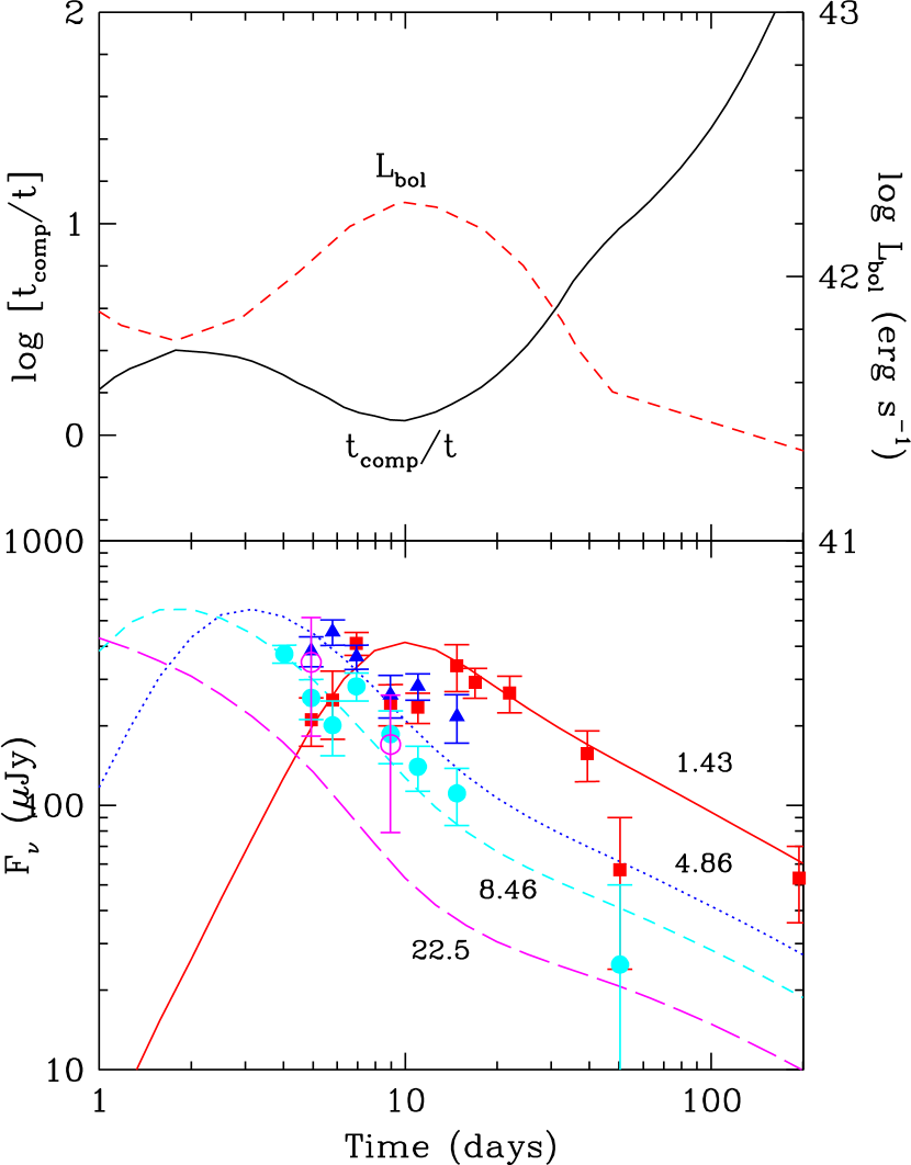
Figure 1: Upper panel: The solid line shows the ratio of the Compton cooling time scale for electrons radiating at $22.5$ GHz to the adiabatic time scale as function of time for the model in the lower panel. The dashed line gives the bolometric luminosity taken from Mazzali et al. (2002), Yoshii et al. (2003), and Pandey et al. (2003). Lower panel: Radio light curves for SN 2002ap. Parameters are given in the text. The observational VLA data are from BKC ($1.43$ GHz–squares; $4.86$ GHz–triangles; $8.46$ GHz–filled circles; $22.5$ GHz–open circles).

When Compton cooling is strong (i.e., $t_{\rm comp}\ll t$), the light curves for the optically thin frequencies are likely to show a minimum close to where the maximum of $L_{\rm bol}$ occurs. In cases where also the optically thick-thin transition is observed, this would give rise to a double peaked structure. The observed time variation of $L_{\rm bol}$ is shown in Figure 1. It is seen that the bolometric luminosity actually peaks during the main radio observing period. Although the observations span a rather limited range in time and, furthermore, are likely to be affected by interstellar scattering and scintillation (BKC), it is noteworthy that no pronounced minimum is apparent in the light curves for the optically thin frequencies. This can be understood if $t_{\rm comp}$ is roughly equal to $t$. Before making a more detailed numerical fit to the data, we will show that if $t_{\rm comp}\sim t$ we can obtain a consistent and plausible set of values for $v_{\rm sh}$, $\epsilon_{\rm B}$ and $\epsilon_{\rm rel}$.

The time scale for Compton cooling is given by

$$t_{\rm comp}=6.6\frac{B^{1/2}}{\nu_{10}^{1/2}U_{\rm ph}}~{}\rm days.$$ (14)

With the use of

$$U_{\rm ph}=4.0\times 10^{-1}\frac{L_{\rm bol,42}}{t_{d}^{2}}\left(\frac{v_{\rm sh}}{c}\right)^{-2}~{}\rm ergs~{}cm^{-3},$$ (15)

the condition $t_{\rm comp}\sim t$ results in

$$L_{\rm bol,42}\sim 10\,B^{1/2}\left(\frac{3v_{\rm sh}}{c}\right)^{2},$$ (16)

where $L_{\rm bol,42}\equiv L_{\rm bol}/10^{42}\rm~{}erg~{}s^{-1}$. Furthermore, $\nu_{10}=1$ and $t=6$ days have been used. As an illustration we show in Figure 1 the ratio of the Compton cooling time scale to the adiabatic time scale for the specific model in §3 with $\dot{M}=10^{-5}~{}M_{\odot}~{}\rm yr^{-1}$, $v_{\rm w}=1000\rm~{}km~{}s^{-1}$, $v_{\rm sh}(t_{\rm d}=10)=70,000\rm~{}km~{}s^{-1}$, and $\epsilon_{\rm B}=10^{-3}$. For other values $t_{\rm comp}\propto(\epsilon_{\rm B}\dot{M}/v_{\rm w})^{1/4}v_{\rm sh}^{2}t^{3/2}L_{\rm bol}^{-1}\nu_{10}^{-1/2}$.

An X-ray flux was detected from SN 2002ap by XMM-Newton on 2002, Feb 3 ($t\approx 6$ days) (Soria & Kong, 2002; Sutaria, Chandra, Bhatnagar, & Ray, 2003; Soria, Pian, & Mazzali, 2004). Due to the weak signal neither the total flux nor the spectral shape could be well determined. The uncertainty in the high energy flux is affected by the subtraction of the flux from a strong, nearby source with a hard spectrum, while at low energy the inability to constrain absorption in excess of the galactic value makes the observed flux a lower limit to the intrinsic one. The observations can be fitted either with a thermal or a power law spectrum. In the latter case, the deduced spectral index is consistent with that observed in the radio. It is therefore likely that the X-ray flux is the Compton scattered optical radiation from the supernova. If this is the case, independent estimates of the energy densities in magnetic fields ($U_{\rm B}$) and relativistic electrons ($U_{\rm rel}$) can be obtained. Since $p\approx 2$

$$\frac{F_{\rm radio}}{F_{\rm X}}\sim\frac{U_{\rm B}}{U_{\rm ph}},$$ (17)

where $F_{\rm radio}\approx\nu F_{\nu}$ is the monochromatic optically thin synchrotron flux and $F_{\rm X}$ is the corresponding X-ray flux. As it turns out, the deduced value of $B$ is such that the same electrons, roughly, are producing both the radio and X-ray fluxes. Hence, equation (17) is not sensitive to the exact value of $p$. Assuming no intrinsic absorption and a power law spectrum with a spectral index consistent with that in the radio give at $t\approx 6$ days a monochromatic X-ray flux $F_{\rm X}\approx(3.0\pm 0.5)\times 10^{-15}~{}\rm ergs~{}cm^{-2}~{}s^{-1}$. At the same time, $F_{\rm radio}\approx 2.0\times 10^{-17}\rm ergs~{}cm^{-2}~{}s^{-1}$ and one finds from equation (17)

$$U_{\rm B}\sim 6\times 10^{-4}L_{\rm bol,42}\left(\frac{3v_{\rm sh}}{c}\right)^{-2}~{}\rm ergs~{}cm^{-3}.$$ (18)

If now $t_{\rm comp}\sim t$, equations (16) and (18) lead to $U_{\rm B}\sim 6\times 10^{-3}B^{1/2}$; hence, $B\sim 0.3~{}\rm G$ and $U_{\rm B}\sim 3\times 10^{-3}~{}\rm ergs~{}cm^{-3}$. Together with the observed value $L_{\rm bol,42}\approx 1.6$ at $t\approx 6$ days, this implies $v_{\rm sh}/c\sim 0.2$.

With a supernova distance $7.3$ Mpc, the observed X-ray flux corresponds to a monochromatic X-ray luminosity $L_{\rm X}\approx 1.9\times 10^{37}\rm~{}erg~{}s^{-1}$, from which the energy density in relativistic electrons is obtained as (cf. eq. [1])

$$U_{\rm rel}\sim\frac{4~{}L_{\rm X}\ln(\gamma_{\rm max}/\gamma_{\rm min})}{\pi v_{\rm sh}^{3}t^{2}},$$ (19)

where, again, the logarithmic factor is due to $p\approx 2.0$. Furthermore, equation (19) assumes $t_{\rm comp}\sim t$ so that, roughly, half of the injected energy emerges as X-ray flux and that, in turn, half of this is emitted through the forward shock (the other half being absorbed by the supernova ejecta). Hence, at $t=6$ days, $U_{\rm rel}\sim 1\times 10^{-4}(3v_{\rm sh}/c)^{-3}\ln(\gamma_{\rm max}/\gamma_{\rm min})~{}\rm ergs~{}cm^{-3}$. With the use of $v_{\rm sh}/c\sim 0.2$, this leads to $U_{\rm rel}\sim 5\times 10^{-4}\ln(\gamma_{\rm max}/\gamma_{\rm min})~{}\rm ergs~{}cm^{-3}$.

Since the unknown values of $\gamma_{\rm max}$ and $\gamma_{\rm min}$ enter only logarithmically in $U_{\rm rel}$, this shows that in the Compton cooling scenario for SN 2002ap, where the relativistic electrons cool on the external photons from the supernova itself, $U_{\rm B}\sim U_{\rm rel}$, i.e., there is rough equipartition between the energy densities in magnetic fields and relativistic electrons. However, both of these energy densities are considerably smaller than that in thermal particles $\epsilon_{\rm B}(\sim\epsilon_{\rm rel})\sim 1\times 10^{-3}(\dot{M}_{-5}/v_{\rm w,3})^{-1}$, unless the mass loss rate of the progenitor is small. The actual values of $U_{\rm B}$ and $U_{\rm rel}$ deduced above are roughly the same as those derived by BKC using radio data alone (in particular, the observed value of the synchrotron self-absorption frequency) and assuming equipartition. The fact that these two independent methods to determine the energy densities in magnetic fields and relativistic electrons give the same value lends support to the Compton cooling scenario. This is further strengthened by the determination of the shock velocity, for which both methods give approximately the same value.

Internally produced synchrotron photons are unlikely to contribute to the cooling as can be seen from the following argument. When cooling is important and $p\approx 2.0$, the energy density of synchrotron photons is $U_{\rm ph}\sim U_{\rm B}(v_{\rm sh}/c)(\epsilon_{\rm rel}/\epsilon_{\rm B})^{1/2}$. The condition corresponding to equation (8) then becomes $\epsilon_{\rm rel}(\dot{M}_{-5}/v_{\rm w,3})>4.7(v_{\rm sh}/c)^{-4/3}(\epsilon_{\rm rel}/\epsilon_{\rm B})^{1/3}$. Since $\epsilon_{\rm rel}/\epsilon_{\rm B}>1$ is necessary for Compton scattering to dominate synchrotron radiation, this requires an even higher mass loss rate than the synchrotron cooling scenario.

3 A model fit to the radio and X-ray radiation of SN 2002ap

The estimates above show that Compton cooling can provide a natural scenario for SN 2002ap. A more detailed model fit to the observations is therefore warranted. We have for this purpose used the numerical model in Fransson & Björnsson (1998), which solves the radiative transfer equation for the synchrotron radiation, including self-absorption, together with the kinetic equation for the electron distribution, including synchrotron, Compton and Coulomb losses. The latter is unimportant for SN 2002ap. As discussed above, we assume that a constant fraction, $\epsilon_{\rm B}$, of the thermal energy behind the shock goes into magnetic fields and a fraction, $\epsilon_{\rm rel}$, into relativistic electrons. The other important input parameters are $p$, $\dot{M}/v_{\rm w}$, and $n$, the ejecta density power law index (specifying the shock velocity, see above). Finally, the bolometric luminosity, $L_{\rm bol}$, determines the Compton cooling. For $L_{\rm bol}$ we use the bolometric light curve determined by Mazzali et al. (2002), Yoshii et al. (2003), and Pandey et al. (2003). Because free-free absorption is unimportant in the cases we consider, and the synchrotron self-absorption is determined by $B$, $n_{\rm rel}$ and $R$ only, $\dot{M}/v_{\rm w}$ always enters in the combination $\epsilon_{\rm B}\dot{M}/v_{\rm w}$ and $\epsilon_{\rm rel}\dot{M}/v_{\rm w}$, reducing the number of free parameters by one, but also preventing us from determining $\dot{M}/v_{\rm w}$ separately.

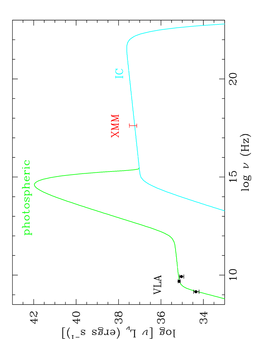
Figure 2: Spectrum ($\nu L_{\nu}$) of SN 2002ap 6 days after explosion. The radio fluxes are from BKC, while the X-ray flux is derived from XMM-observations (see text for a discussion of the uncertainties associated with this value).

Using this model, we have varied the parameters to give a best fit of the radio light curves together with the XMM flux at 6 days, taken from Sutaria, Chandra, Bhatnagar, & Ray (2003). In Figure 1 we show the resulting light curves and in Figure 2 the full spectrum at 6 days, together with the VLA and XMM observations. In this figure we have also added the luminosity from the supernova photosphere. The latter can on day 6 be well approximated as a black-body with temperature of $\sim 5000$ K and a total luminosity of $1.6\times 10^{42}\rm~{}erg~{}s^{-1}$ (Pandey et al., 2003). As input electron spectrum we use $p=2.1$, and $\gamma_{\rm min}=1$ and $\gamma_{\rm max}=5\times 10^{3}$. The latter is only important for the upper energy limit of the gamma-ray flux from inverse Compton.

In order to reproduce the decrease in the optically thin parts of the light curves, the best fit model has $n=10$, in agreement with the expected density structure for the progenitor of an Ic SN (Matzner & McKee, 1999). This is also consistent with hydrodynamical models of Type Ic supernovae, where the power law index varies between $n=8$ and $n=13$ for ejecta velocities above $\sim 25,000\rm~{}km~{}s^{-1}$ (Iwamoto et al., 2000).The expansion velocity we find is $70,000\rm~{}km~{}s^{-1}$ at 10 days, somewhat lower than deduced by BKC. As discussed in §2.2, the requirement that inverse Compton scattering should reproduce both the X-ray flux and the synchrotron radio spectrum, sets the value of $\epsilon_{\rm B}/\epsilon_{\rm rel}$ as well as $\epsilon_{\rm B}\dot{M}/v_{\rm w}$, and we find that $\epsilon_{\rm B}/\epsilon_{\rm rel}\approx 0.2$ and $\epsilon_{\rm B}\dot{M}/v_{\rm w}\approx 1\times 10^{-11}~{}M_{\odot}~{}\rm yr^{-1}/\rm~{}km~{}s^{-1}$. Note that $\epsilon_{\rm rel}$ is roughly proportional to $\ln(\gamma_{\rm max}/\gamma_{\rm min})$. Since the values of both $\gamma_{\rm min}$ and $\gamma_{\rm max}$ are unknown, this introduces an uncertainty in the value of $\epsilon_{\rm rel}$; for example, using $\gamma_{\rm min}=\gamma_{\rm abs}$, where $\gamma_{\rm abs}$ is the Lorentz factor of the electrons radiating at the synchrotron self-absorption frequency, yields $\epsilon_{\rm B}/\epsilon_{\rm rel}\approx 1$. As anticipated in §2.2, inverse Compton cooling of the electrons is important, leading to a steepening of the electron spectrum and a spectral flux $F_{\nu}\propto\nu^{-0.9}$, in agreement with observations (BKC). The importance of Compton cooling for the calculated light curves can be seen especially at high frequencies, where the cooling time is comparable to the dynamical time (cf. Fig. 1). For these a depression is apparent at the time of maximum Compton cooling at $\approx 10$ days.

4 Discussion

In order to derive the main parameters characterizing an observed synchrotron source of unknown size, one often has to invoke the assumption of equipartition between energies in relativistic electrons and magnetic field (i.e., $\epsilon_{\rm B}\approx\epsilon_{\rm rel}$). The independent determination of these quantities requires either that radiative cooling is important within the observed frequency range, or that the Compton scattered radiation is observed. In the latter case, the scattered radiation can be the synchrotron photons themself or come from a known external source of photons.

We have shown in this paper that the radio, optical and X-ray observations of SN 2002ap can be understood in a scenario, wherein the relativistic electrons cool by inverse Compton scattering on the photospheric supernova photons and thereby giving rise to the X-ray emission. Since both radiative cooling and the Compton scattered emission are observed, not only can a value for $\epsilon_{\rm B}/\epsilon_{\rm rel}$ be derived but, in addition, an internal consistency check of the model can be made; for example, the value of the synchrotron self-absorption frequency can be predicted. The Compton cooling scenario implies rough equipartition conditions in SN 2002ap. Furthermore, the actual value deduced for $\epsilon_{\rm B}$ ($\sim\epsilon_{\rm rel}$) is close to the one derived by BKC from the observed values of the synchrotron self-absorption frequency and flux assuming equipartition. This shows that the model self-consistently predicts the frequency of the synchrotron self-absorption, as was illustrated in §3.

There is, however, one underlying assumption; namely, a spherically symmetric source. It is seen in §2.2 that the only place where the assumption of a spherically symmetric source geometry enters is in the derivation of the energy density of relativistic electrons from the observed X-ray luminosity (cf. eq. [19]). Deviations from spherical symmetry, for example a jet structure, would then have to be compensated for by an increased energy density of relativistic electrons. Since the deduced values of $B$ and $v_{\rm sh}$ are not affected (cf. eqs. [16] and[18]), this results in an increased synchrotron self-absorption frequency. Due to the short term flux variations, which are likely caused by interstellar scattering and scintillation, the limits of the allowed variations of the predicted self-absorption frequency are hard to evaluate precisely. From the early observations at the lowest frequency (1.43 GHz), when the radiation at this frequency was optically thick, it seems unlikely that the observed self-absorption frequency has been underestimated by more than a factor two. Since synchrotron self-absorption frequency scales with energy density of relativistic electrons as $\epsilon_{\rm rel}^{2/(p+4)}$, the value of $\epsilon_{\rm rel}$ can be increased at most by a factor ten. Hence, the solid angle of a jet has to cover at least 10 % of the sky. This conclusion is similar to the one reached by Totani (2003), using a different line of reasoning.

BKC argue that the observed XMM flux can be described as an extrapolation of the synchrotron flux. This is apparently based on the assumption that the radio spectral index is close to $\beta\sim 0.5$, which is needed to explain the light curves in the absence of cooling. The resulting spectral break in the optical frequency range due to synchrotron cooling in an equipartition magnetic field would give rise to an X-ray flux and spectral index in approximate agreement with those observed. However, as discussed in §2.2, the observed spectral index in the radio is $\beta\sim 0.9$, which is similar to that in the X-ray range, making this scenario untenable.

Sutaria, Chandra, Bhatnagar, & Ray (2003) explain the X-ray flux as a result of thermal inverse Compton scattering by the thermal electrons behind the shock (see Fransson, 1982). In order to have sufficient electron optical depth, they need to have the X-ray emitting region moving with a velocity $\sim 16,000\rm~{}km~{}s^{-1}$. A similar low velocity of the forward shock is needed in the model by Soria, Pian, & Mazzali (2004). They argue that the X-ray emission is free-free emission from the reverse shock. There are several features of these models which make them less attractive. In the thermal inverse Compton scattering model, the spectral index is very sensitive both to shock temperature and optical depth. The low shock temperature in the free-free model requires a density structure of the ejecta corresponding to $n\sim 40$ at velocities $\sim 10,000-20,000\rm~{}km~{}s^{-1}$, which is quite different from that thought appropriate fora Ic SN, $n\lesssim 10$ (Iwamoto et al., 2000; Matzner & McKee, 1999), in this velocity range.

In addition to these model specific problems, there are two rather model independent arguments against any model invoking such low shock velocities. First, the line emission observed in SN 2002ap should set a lower limit to the velocity of the forward shock. Due to line blending, accurate velocities were hard to measure in SN 2002ap. However, it seems clear that velocities of at least $0.1~{}\rm c$ are indicated. Mazzali et al. (2002) find in their first spectrum at 2 days a photospheric velocity of 30,000 km/s, and at 3.5 days 20,500 km/s. It is important to note that this is the velocity where the continuum is becoming optically thick and, therfore, provides a lower limit to the velocity of the line emitting regions. This is confirmed by the observations of Foley et al. (2003), which show that the P-Cygni profile of the O I $\lambda 7774$ line on day 15 extends at least to $\sim 24,000\rm~{}km~{}s^{-1}$, where it becomes blended with other lines. This, in turn, should be a conservative lower limit to the shock velocity and, hence, calls in question the consistency of the proposed models.

Another issue for low velocity models is the incorporation of the observed radio emission. Assuming the radio emission to come from behind the forward and/or the reverse shock, implies a brightness temperature which scales, roughly, as $v_{\rm sh}^{-2}$. The low shock velocities argued for in the above two models result in brightness temperatures about a factor 10 larger than the Compton limit. This, in turn, would produce an X-ray flux much in excess to that observed.

The rough equipartion between the energies in relativistic electrons and magnetic fields found for SN 2002ap is in sharp contrast to the conditions in SN 1993J for which $\epsilon_{\rm B}/\epsilon_{\rm rel}\gg 1$ was deduced by Fransson & Björnsson (1998). Unfortunately, these are the only two SNe for which an independent estimate of $\epsilon_{\rm B}/\epsilon_{\rm rel}$ has been possible to make. In this context it is interesting to note that for the afterglows of GRBs the deduced values of $\epsilon_{\rm B}/\epsilon_{\rm rel}$ exhibit a large range (e.g., Panaitescu & Kumar, 2002). However, there is a clear tendency for this ratio to be smaller, or for some afterglows much smaller, than unity. Although the conditions for both magnetic field generation and particle acceleration may differ considerably between relativistic and non-relativistic shocks, a plausible cause for the substantial difference in the value of $\epsilon_{\rm B}/\epsilon_{\rm rel}$ behind the non-relativistic shocks in SN 1993J and SN 2002ap is harder to find.

5 Conclusions

We have shown that in SN 2002ap inverse Compton scattering of the photospheric photons is important for those relativistic electrons producing the radio emission. The scattering cools the relativistic electrons, and gives rise to an X-ray flux which matches the observed flux level as well as the spectral index. The value for the shock velocity, $\sim 70,000\rm~{}km~{}s^{-1}$, is in rough agreement with BKC. The deduced energy densities in magnetic fields and relativistic electrons are close to equipartition. However, without a priori knowledge of what fraction of the total injected energy density these quantities correspond to, no estimate can be made of the mass loss rate of the progenitor star. From the radio and X-ray observations the mass loss rate can be constrained to $\dot{M}\approx 1\times 10^{-8}(v_{\rm w}/1000\rm~{}km~{}s^{-1})\epsilon_{\rm B}^{-1}~{}M_{\odot}~{}\rm yr^{-1}$. BKC assumed $\epsilon_{\rm B}=\epsilon_{\rm rel}=0.1$, which would imply $\dot{M}\approx 1\times 10^{-7}(v_{\rm w}/1000\rm~{}km~{}s^{-1})~{}M_{\odot}~{}\rm yr^{-1}$; this is very low for a Wolf-Rayet star. Turning this argument around, a typical Wolf-Rayet mass loss rate of $\dot{M}\sim 10^{-5}~{}M_{\odot}~{}\rm yr^{-1}$ and wind velocity of $\sim 2000\rm~{}km~{}s^{-1}$, would imply $\epsilon_{\rm B}\sim 2\times 10^{-3}$.

An important conclusion from this paper is that any self-consistent model of the radio and X-ray flux observed from SN 2002ap needs to include effects due to the photospheric emission. It is likely that in any SNe, for which the synchrotron emission from behind the shock becomes transparent not too long after the photospheric emission has reached its maximum, inverse Compton scattering can be an important factor shaping the radio and/or X-ray spectrum. Another outcome of our analysis is that the time variation of the radio emission allows a determination of the density structure of the ejecta. It is reassuring that the result is close to what is expected theoretically.

References

- Berger, Kulkarni, & Chevalier (2002) Berger, E., Kulkarni, S. R., & Chevalier, R. A. 2002, ApJ, 577, L5
- Chevalier (1982) Chevalier, R. A. 1982, ApJ, 258, 790
- Chevalier & Fransson (2003) Chevalier, R. A. & Fransson, C. 2003, in ”Supernovae and Gamma-Ray Bursts,” edited by K. W. Weiler (Springer-Verlag), 171
- Chevalier & Li (2000) Chevalier, R. A. & Li, Z. 2000, ApJ, 536, 195
- Foley et al. (2003) Foley, R. J. et al. 2003, PASP, 115, 1220
- Fransson (1982) Fransson, C. 1982, A&A, 111, 140
- Fransson & Björnsson (1998) Fransson, C. & Björnsson, C.-I. 1998, ApJ, 509, 861
- Hjorth et al. (2003) Hjorth, J., et al. 2003, Nature, 423, 847
- Iwamoto et al. (2000) Iwamoto, K. et al. 2000, ApJ, 534, 660
- Iwamoto et al. (2003) Iwamoto, K., Nomoto, K., Mazzali, P. A., Nakamura, T., & Maeda, K. 2003, in ”Supernovae and Gamma-Ray Bursts,” edited by K. W. Weiler (Springer-Verlag), 243
- Kawabata et al. (2003) Kawabata, K. S. et al. 2003, ApJ, 593, L19
- Li & Chevalier (2003) Li, Z. & Chevalier, R. A. 2003, in ”Supernovae and Gamma-Ray Bursts,” edited by K. W. Weiler (Springer-Verlag), 419
- Lundqvist & Fransson (1988) Lundqvist, P. & Fransson, C. 1988, A&A, 192, 221
- Matzner & McKee (1999) Matzner, C. D. & McKee, C. F. 1999, ApJ, 510, 379
- Mazzali et al. (2002) Mazzali, P. A. et al. 2002, ApJ, 572, L61
- Nomoto et al. (1994) Nomoto, K., Yamaoka, H., Pols, O. R., van den Heuvel, E. P. J., Iwamoto, K., Kumagai, S., & Shigeyama, T. 1994, Nature, 371, 227
- Panaitescu & Kumar (2002) Panaitescu, A. & Kumar, P. 2002, ApJ, 571, 779
- Pandey et al. (2003) Pandey, S. B., Anupama, G. C., Sagar, R., Bhattacharya, D., Sahu, D. K., & Pandey, J. C. 2003, MNRAS, 340, 375
- Sharina, Karachentsev, & Tikhonov (1996) Sharina, M. E., Karachentsev, I. D., & Tikhonov, N. A. 1996, A&AS, 119, 499
- Soria & Kong (2002) Soria, R. & Kong, A. K. H. 2002, ApJ, 572, L33
- Soria, Pian, & Mazzali (2004) Soria, R., Pian, E., & Mazzali, P. A. 2004, A&A, 413, 107
- Stanek et al. (2003) Stanek, K. Z. et al. 2003, ApJ, 591, L 17