Likelihood analysis of the Local Group acceleration revisited

Abstract

We reexamine likelihood analyzes of the Local Group (LG) acceleration, paying particular attention to nonlinear effects. Under the approximation that the joint distribution of the LG acceleration and velocity is Gaussian, two quantities describing nonlinear effects enter these analyzes. The first one is the coherence function, i.e. the cross-correlation coefficient of the Fourier modes of gravity and velocity fields. The second one is the ratio of velocity power spectrum to gravity power spectrum. To date, in all analyzes of the LG acceleration the second quantity was not accounted for. Extending our previous work, we study both the coherence function and the ratio of the power spectra. With the aid of numerical simulations we obtain expressions for the two as functions of wavevector and $\sigma_{8}$. Adopting WMAP’s best determination of $\sigma_{8}$, we estimate the most likely value of the parameter $\beta$ and its errors. As the observed values of the LG velocity and gravity, we adopt respectively a CMB-based estimate of the LG velocity, and Schmoldt et al.’s (1999) estimate of the LG acceleration from the PSCz catalog. We obtain $\beta=0.66^{+0.21}_{-0.07}$; thus our errorbars are significantly smaller than those of Schmoldt et al. This is not surprising, because the coherence function they used greatly overestimates actual decoherence between nonlinear gravity and velocity.

1 Introduction

Analyzes of large-scale structure of the Universe provide estimates of cosmological parameters that are complementary to those from the cosmic microwave background (CMB) measurements. In particular, comparing the large-scale distribution of galaxies to their peculiar velocities enables one to constrain the quantity $\beta\equiv\Omega_{m}^{0.6}/b$. Here, $\Omega_{m}$ is the cosmological matter density parameter and $b$ is the linear bias of galaxies that are used to trace the underlying mass distribution. This is so because the peculiar velocity field, ${\bf v}$, is induced gravitationally and therefore is tightly coupled to the matter distribution. In the linear regime, this relationship takes the form

$${\bf v}=\Omega_{m}^{0.6}\int\frac{{\rm d}^{3}{\bf r}}{4\pi}\delta({\bf r})\frac{{\bf r}}{r^{3}}\,,$$ (1)

where $\delta$ denotes the mass density contrast and distances have been expressed in $\hbox{km}\cdot\hbox{s}^{-1}$. Under the assumption of linear bias $\delta=b^{-1}\delta_{g}$, where $\delta_{g}$ denotes the density contrast of galaxies, and the amplitude of peculiar velocities depends linearly on $\beta$.

These comparisons are done by extracting the density field from full-sky redshift surveys (such as the PSCz; Saunders et al. 2000), and comparing it to the observed velocity field from peculiar velocity surveys. The methods for doing this fall into two broad categories. One can use equation (1) to calculate the predicted velocity field from a redshift survey, and compare the result with the measured peculiar velocity field; this is referred to as a velocity–velocity comparison. Alternatively, one can use the differential form of this equation, and calculate the divergence of the observed velocity field to compare directly with the density field from a redshift survey; this is called a density–density comparison.

Peculiar velocities of galaxies and groups of galaxies are generally determined by measuring their distances independently of redshifts. However, the motion of the Local Group (LG) of galaxies can be deduced in another way, namely from the observed dipole anisotropy of the CMB temperature. This dipole reflects, via the Doppler shift, the motion of the Earth with respect to the CMB rest frame. The components of this motion of local, non-cosmological origin (the Earth motion around the Sun, the Sun motion in the Milky Way and the motion of the Milky Way in the LG) are known and can be subtracted (e.g., Courteau & van den Bergh 1999). When transformed to the barycenter of the LG, the motion is towards $(l,b)=(276^{\circ}\pm 3^{\circ},30^{\circ}\pm 2^{\circ})$, and of amplitude $v_{\rm LG}=627\pm 22$ $\hbox{km}\cdot\hbox{s}^{-1}$, as inferred from the 4-year COBE data (Lineweaver et al. 1996). It can be compared to that predicted from a redshift survey and historically this was the first velocity–velocity comparison (with angular data only, e.g. Meiksin & Davis 1986, Yahil, Walker & Rowan-Robinson 1986; with redshift information, Strauss & Davis 1988, Lynden-Bell, Lahav & Burstein 1989). This velocity estimate is much more accurate than estimates of peculiar velocities based on redshift-independent distances. Therefore, the analysis of the LG motion remains an interesting alternative to current velocity–velocity comparisons, performed simultaneously for many galaxies, but with less accurately measured velocities.

Let us define the scaled gravity, ${\bf g}$, by the equation:

$${\bf g}=\int\frac{{\rm d}^{3}{\bf r}}{4\pi}\delta({\bf r})\frac{{\bf r}}{r^{3}}\,,$$ (2)

where again distances have been expressed in $\hbox{km}\cdot\hbox{s}^{-1}$. The scaled gravity is proportional to the gravitational acceleration, and can be measured from a redshift survey. Equation (1) yields

$${\bf v}=\Omega_{m}^{0.6}{\bf g}\,,$$ (3)

so a velocity–velocity comparison is in fact a velocity–gravity one. Hereafter, we will refer to ‘scaled gravity’ simply by ‘gravity’. It is also often called ‘the clustering dipole’.

A number of effects (nonlinear effects, observational windows through which the velocity and gravity of the LG are observed, shot noise) spoil the linear relationship (3). Therefore, to estimate $\beta$ one cannot simply equate the two dipoles, but a more sophisticated approach is needed. Commonly adopted is a maximum likelihood approach, which provides a way to account for these effects and to compute errors of estimated cosmological parameters. Here we reexamine a likelihood analysis of Schmoldt et al. (1999; S99), paying particular attention to proper modelling of nonlinear effects (NE), that affect the estimated values of parameters and their errors.

In a previous work (Chodorowski & Cieciela̧g 2002; hereafter C02) we concentrated on one quantity describing NE in the LG velocity–gravity comparison, the coherence function (CF). It is the cross-correlation coefficient of the Fourier modes of the gravity and velocity fields. We showed that the form of the function adopted by S99 drastically overestimates actual decoherence between nonlinear gravity and velocity. This implies that the true random error of $\beta$ is significantly smaller. In the present study we give a complete description of NE present in the analysis. In particular, we show that not only the CF is relevant, but also the ratio of the power spectrum of velocity to the power spectrum of gravity. With aid of numerical simulations we model the two quantities as functions of the wavevector and of cosmological parameters. We then combine these results with observational estimates of ${\bf v}_{\rm LG}$ and ${\bf g}_{\rm LG}$, and obtain the ‘best’ value of $\beta$ and its errors. The paper is organized as follows. In Section 2 we outline an analytical description of the likelihood for cosmological parameters, based on the measured values of the LG velocity and acceleration. In Section 3 we describe our numerical simulations, and we model numerically the coherence function and the ratio of the power spectra. An estimation of the most likely value of $\beta$ and its errors is presented in Section 4. Summary and conclusions are in Section 5.

2 Analytical description of the likelihood

Let $f({\bf g},{\bf v})$ denote the joint distribution function for the LG gravity and velocity. It is commonly approximated by a multivariate Gaussian (Strauss et al. 1992, hereafter S92; S99). This approximation has support from numerical simulations (Kofman et al. 1994, Cieciela̧g et al. 2003), where the measured nongaussianity of ${\bf g}$ and ${\bf v}$ is small. This is rather natural to expect since, e.g., gravity is an integral of density over effectively a large volume, so the central limit theorem can at least partly be applicable (but see Catelan & Moscardini 1994).

In a Bayesian approach, one ascribes a priori equal probabilities to values of unknown parameters, which allows one to express their likelihood function via $f$:

$$\mathcal{L}(\rm param.)=f({\bf v},{\bf g}~{}|~{}\rm param.)\,.$$ (4)

As the parameters to be estimated we adopt $\beta$ and $b$. Using statistical isotropy of ${\bf g}$ and ${\bf v}$, the distribution function can be cast to the form (Juszkiewicz et al. 1990, Lahav, Kaiser & Hoffman 1990):

$$f({\bf g},{\bf v})=\frac{(1-r^{2})^{-3/2}}{(2\pi)^{3}\sigma_{\bf g}^{3}\sigma_{\bf v}^{3}}\exp\left[-\frac{x^{2}+y^{2}-2r\mu xy}{2(1-r^{2})}\right]\,,$$ (5)

where $\sigma_{\bf g}$ and $\sigma_{\bf v}$ are the r.m.s. values of a single Cartesian component of gravity and velocity, respectively. From isotropy, $\sigma_{\bf g}^{2}=\langle{\bf g}\cdot{\bf g}\rangle/3$, and $\sigma_{\bf v}^{2}=\langle{\bf v}\cdot{\bf v}\rangle/3$, where $\langle\cdot\rangle$ denote the ensemble averaging. Next, $({\bf x},{\bf y})=({\bf g}/\sigma_{\bf g},{\bf v}/\sigma_{\bf v})$, and $\mu=\cos\psi$ with $\psi$ being the misalignment angle between ${\bf g}$ and ${\bf v}$. Finally, $r$ is the cross-correlation coefficient of $g_{m}$ with $v_{m}$, where $g_{m}$ ($v_{m}$) denotes an arbitrary Cartesian component of ${\bf g}$ (${\bf v}$). From isotropy,

$$r=\frac{\langle{\bf g}\cdot{\bf v}\rangle}{\langle g^{2}\rangle^{1/2}\langle v^{2}\rangle^{1/2}}\,.$$ (6)

Also from isotropy,

$$\langle x_{m}y_{n}\rangle=r\,\delta_{mn}\,,$$ (7)

where $\delta_{mn}$ denotes the Kronecker delta. In other words, there are no cross-correlations between different spatial components.

We have to take into account that the LG gravity is measured through the window $W_{\bf g}$:

$${\bf g}=\int\frac{{\rm d}^{3}r}{4\pi}\delta({\bf r})W_{\bf g}(r)\frac{{\bf r}}{r^{3}}\,.$$ (8)

If ${\bf v}$ is irrotational like ${\bf g}$, then similarly

$${\bf v}=\int\frac{{\rm d}^{3}r}{4\pi}\theta({\bf r})W_{\bf v}(r)\frac{{\bf r}}{r^{3}}\,,$$ (9)

where $\theta$ is the (minus) velocity divergence, $\theta\equiv-\nabla\cdot{\bf v}$, and $W_{\bf v}$ is the velocity window. Due to Kelvin’s circulation theorem, the cosmic velocity field is vorticity-free as long as there is no shell crossing. N-body simulations (Bertshinger & Dekel 1989, Mancinelli et al. 1994, Pichon & Bernardeau 1999) show that the vorticity of velocity is small in comparison to its divergence even in the fully nonlinear regime.

The best current estimate of the LG gravity is inferred from the PSCz catalog of IRAS galaxies (Saunders et al. 2000). S99 follow S92 and measure the LG gravity through the standard IRAS window,

$$W_{\bf g}=\left\{\begin{array}[]{ll}(r/r_{s})^{3},&r<r_{s}\,,\\ 1,&r_{s}<r<R_{\rm max}\,,\\ 0,&R_{\rm max}<r\,.\end{array}\right.$$ (10)

The window is characterized by a small-scale smoothing and a sharp large-scale cutoff. Following S99, we adopt the values $r_{s}=500$ $\hbox{km}\cdot\hbox{s}^{-1}$ and $R_{\rm max}=15,000$ $\hbox{km}\cdot\hbox{s}^{-1}$, appropriate for the PSCz catalog. The window function relevant to the LG velocity is

$$W_{\bf v}=\left\{\begin{array}[]{ll}0,&r<r_{\rm min}\,,\\ 1,&\mbox{otherwise}\,,\end{array}\right.$$ (11)

which has a small-scale cutoff, $r_{\rm min}=100$ $\hbox{km}\cdot\hbox{s}^{-1}$, to reflect the finite size of the LG (S92). Using numerical simulations, we have checked that the velocity field remains approximately Gaussian even for such a small smoothing scale.

In Fourier space, relations (8) and (9) read:

$${\bf g}_{{\bf k}}=\frac{i{\bf k}}{k^{2}}\delta_{{\bf k}}\widehat{W}_{g}(k),$$ (12)

$${\bf v}_{{\bf k}}=\frac{i{\bf k}}{k^{2}}\theta_{{\bf k}}\widehat{W}_{v}(k),$$ (13)

where the subscript ${\bf k}$ denotes the Fourier transform. The quantity $\widehat{W}$ is not a Fourier transform of $W$, but is related to it in the following way (S92):

$$\widehat{W}(k)\equiv k\!\int_{0}^{\infty}\!W(r)j_{1}(kr)dr\,.$$ (14)

Here and below $j_{l}$ represents the spherical Bessel function of order $l$. In particular,

$$\widehat{W}_{g}(k)=\frac{3j_{1}(kr_{s})}{kr_{s}}-j_{0}(kR_{\rm max})\,,$$ (15)

and

$$\widehat{W}_{v}(k)=j_{0}(kr_{\rm min})\,.$$ (16)

From equations (12) and (13) we have

$$\langle{\bf g}\cdot{\bf g}\rangle=\frac{1}{2\pi^{2}}\int_{0}^{\infty}\widehat{W}_{\bf g}^{2}(k)P(k)dk\,,$$ (17)

and

$$\langle{\bf v}\cdot{\bf v}\rangle=\frac{1}{2\pi^{2}}\int_{0}^{\infty}\widehat{W}_{\bf v}^{2}(k)P_{\theta}(k)dk\,.$$ (18)

Here, $P(k)$ and $P_{\theta}(k)$ are respectively the power spectrum of the density and the power spectrum of the velocity divergence. Thus,

$$\langle{\bf v}\cdot{\bf v}\rangle=\frac{1}{2\pi^{2}}\int_{0}^{\infty}\widehat{W}_{\bf v}^{2}(k){\cal R}(k)P(k)dk\,,$$ (19)

where

$${\cal R}(k)\equiv\frac{P_{{\bf v}}(k)}{P_{{\bf g}}(k)}=\frac{P_{\theta}(k)}{P(k)}\,,$$ (20)

and $P_{{\bf v}}$ and $P_{{\bf g}}$ are the power spectra respectively of velocity and gravity. Furthermore,

$$\langle{\bf g}\cdot{\bf v}\rangle=\frac{1}{2\pi^{2}}\int_{0}^{\infty}\widehat{W}_{\bf g}(k)\widehat{W}_{\bf v}(k)C(k)P_{\theta}^{1/2}(k)P^{1/2}(k)dk,$$ (21)

where $C(k)$ is the so-called coherence function (S92), or the correlation coefficient of the Fourier components of the gravity and velocity fields:

$$C(k)\equiv\frac{\langle{\bf g}_{\bf k}\cdot{\bf v}_{\bf k}^{\star}\rangle}{\langle|{\bf g}_{\bf k}|^{2}\rangle^{1/2}\langle|{\bf v}_{\bf k}|^{2}\rangle^{1/2}}=\frac{\langle\delta_{\bf k}\theta_{\bf k}^{\star}\rangle}{\langle|\delta_{\bf k}|^{2}\rangle^{1/2}\langle|\theta_{\bf k}|^{2}\rangle^{1/2}}\,.$$ (22)

Hence, we obtain

$$r=\frac{\int_{0}^{\infty}\widehat{W}_{\bf g}(k)\widehat{W}_{\bf v}(k)C(k){\cal R}^{1/2}(k)P(k)dk}{\left[\int_{0}^{\infty}\widehat{W}_{\bf g}^{2}(k)P(k)dk\right]^{1/2}\left[\int_{0}^{\infty}\widehat{W}_{\bf v}^{2}(k){\cal R}(k)P(k)dk\right]^{1/2}}\,.$$ (23)

Equations (17), (19) and (23) specify all parameters (the variances and the correlation coefficient) that determine distribution (5) in the absence of observational errors. The deviation of the correlation coefficient from unity is then due to different windows, through which the gravity and the velocity of the LG are measured, and due to nonlinear effects. The latter are described by two functions: the coherence function, and the ratio of the power spectra. In the linear regime, $C(k)=1$ and ${\cal R}=\Omega_{m}^{1.2}$. This yields

$$r=\frac{\int_{0}^{\infty}\widehat{W}_{\bf g}(k)\widehat{W}_{\bf v}(k)P(k)dk}{\left[\int_{0}^{\infty}\widehat{W}_{\bf g}^{2}(k)P(k)dk\right]^{1/2}\left[\int_{0}^{\infty}\widehat{W}_{\bf v}^{2}(k)P(k)dk\right]^{1/2}}\,,$$ (24)

so for linear fields the correlation coefficient is determined solely by the windows, as expected.

3 Modelling nonlinear effects

3.1 Numerical simulations

We follow the evolution of the dark matter distribution using the pressureless hydrodynamic code CPPA (Cosmological Pressureless Parabolic Advection, see Kudlicki, Plewa & Różyczka 1996, Kudlicki et al. 2000 for details). It employs an Eulerian scheme with third order accuracy in space and second order in time, which assures low numerical diffusion and an accurate treatment of high density contrasts. Standard applications of hydrodynamic codes involve a collisional fluid; however, we implemented a simple flux interchange procedure to mimic collisionless fluid behaviour. Thanks to this approach we avoid a few problems of N-body codes. The main advantage of a hydrodynamic code over an N-body code is accurate treatment of low density regions. Moreover it directly produces a volume-weighted velocity field. This is important because in the definition of the CF, equation (22), the velocity field is volume-weighted, not mass-weighted. Furthermore, the Fast Fourier Transform can be directly applied to the data on an uniform grid.

The computational domain forms a $(400{\,h^{-1}\rm Mpc})^{3}$ cube with $256^{3}$ grid cells and periodic boundary conditions. This setup allows us to cover a broad range of wavenumbers, $k\in[0.016,2.]$ $h/\hbox{Mpc}$, which is important for accurate calculation of the integrals in equation (23). The initial distribution of the density fluctuations is Gaussian and their power spectrum is given by a CDM formula (as in Eq. 7 of Efstathiou, Bond & White 1992) with the shape parameter $\Gamma=0.19$, as inferred from the IRAS PSCz survey (Sutherland et al. 1999) and in agreement with recent determinations from WMAP (Spergel et al. 2003). The initial value of the square root of the variance of the density field in spheres of radius 8 $h^{-1}\,\hbox{Mpc}$, $\sigma_{8}(t_{i})$, is $0.019$. We studied a range of outputs from the simulations, corresponding to different values of $\sigma_{8}$. Specifically, full output data were dumped in constant intervals of the scale factor, $\Delta a=0.025$.

All our simulations assume $\Omega_{m}=0.3$, $\Omega_{\Lambda}=0$. In the mildly non-linear regime, the quantity $\tilde{\bf v}\equiv\Omega_{m}^{-0.6}{\bf v}$ is insensitive to the cosmological density parameter and cosmological constant, as demonstrated both analytically (Bouchet et al. 1995, Nusser & Colberg 1998; see also Appendix B3 of Scoccimarro et al. 1998) and by means of N-body simulations (Bernardeau et al. 1999). Therefore, our results should be valid for any cosmology. Specifically, we have

$${\cal R}=\Omega_{m}^{1.2}\tilde{\cal R}$$ (25)

and

$$C=\tilde{C}\,,$$ (26)

where

$$\tilde{\cal R}(k)=\frac{P_{\tilde{{\bf v}}}(k)}{P_{{\bf g}}(k)}$$ (27)

and

$$\tilde{C}(k)=\frac{\langle{\bf g}_{\bf k}\cdot\tilde{\bf v}_{\bf k}^{\star}\rangle}{\langle|{\bf g}_{\bf k}|^{2}\rangle^{1/2}\langle|\tilde{\bf v}_{\bf k}|^{2}\rangle^{1/2}}\,.$$ (28)

In a previous paper (C02), we tested numerically the dependence of the coherence function on $\Omega_{m}$ and found it to be extremely weak.

In C02, we also investigated numerical effects. In short, we found that the effects of resolution affect numerical determination of the CF at scales smaller than 4 grid cells, ie. twice the Nyquist wavelength. Therefore, all the results we present here are for $k<1$ $h/\hbox{Mpc}$. For these wavenumbers, both simulated $C$ and ${\cal R}$ practically do not depend on resolution. Also, here we use a larger box size than in C02 in order to model longer modes, while the short wavelength limit ($k<1$ $h/\hbox{Mpc}$) still allows us to accurately calculate the integrals in Equation (23), as will be shown in subsection 3.4.

3.2 Coherence function

We studied the CF in C02. We found there that the characteristic decoherence scale is an order of magnitude smaller than previously used (S92). The weak point of the formula fitted in C02 was a poor description of the CF for long-wavelength modes. These modes are however important when calculating integrals in equation (23). (From eqs. 12–13 it follows that the gravity and velocity fields are more sensitive to long-wavelength modes than the density field.) Therefore, here we use another fitting function, which is more accurate for low values of $k$:

$$\tilde{C}(k)=\left[1+(a_{0}k-a_{2}k^{1.5}+a_{1}k^{2})^{2.5}\right]^{-0.2}.$$ (29)

Parameters $a_{l}$ were obtained for 35 different values of $\sigma_{8}$ in the range [0.1,1], and we found the following, power-law, scaling relations:

$$a_{0} = 4.908\ \sigma_{8}^{0.750}$$

$$a_{1} = 2.663\ \sigma_{8}^{0.734}$$ (30)

$$a_{2} = 5.889\ \sigma_{8}^{0.714}.$$

The fit was calculated for $k\in[0,1]$ $h/\hbox{Mpc}$, with the imposed constraint $C(k=0)=1$. Unlike the previous fit, the new one results in the value of the correlation coefficient of gravity and velocity which agrees with that measured directly in our simulations. In Figure 1 we show, for various values of $\sigma_{8}$, the CF from simulations, its fit (29), and results of perturbative calculations, described in C02. We see that the perturbative approximation breaks down for $\sigma_{8}>0.5$.

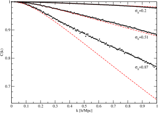
Figure 1: The coherence function for various values of $\sigma_{8}$. Dots show the results of simulations, solid lines – our fit (29), and dashed lines – the results of perturbative calculations. Perturbative approximation breaks down for $\sigma_{8}>0.5$.

3.3 Ratio of the power spectra

The ratio of the velocity to the gravity power spectra, $\mathcal{R}$, is related to its scaled counterpart, $\tilde{\cal R}$, by equation (25). The quantity $\tilde{\cal R}$, defined in equation (27), practically does not depend on the background cosmological model. It departs from unity in the nonlinear regime because the velocity grows slower than it would be expected from the linear approximation.

We have found that $\tilde{\mathcal{R}}$ obtained from simulation can be fitted with the following formula:

$$\tilde{\mathcal{R}}(k)=[1+(7.071k)^{4}]^{-\alpha}\,,$$ (31)

with

$$\alpha=-0.06574+0.29195\sigma_{8}\qquad\mathrm{for}~{}0.3<\sigma_{8}<1\,.$$ (32)

We stress that the above relation between $\alpha$ and $\sigma_{8}$ is valid for $\sigma_{8}\in[0.3,1]$, which is still a sufficiently wide range of values. Figure 2 shows the ratio of the power spectra from simulation, and our fit.

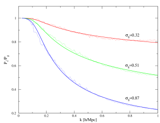
Figure 2: The ratio of the velocity power spectrum to the gravity power spectrum as a function of the wavevector for three different values of $\sigma_{8}$. Dotted lines show the results of our simulations and solid lines – the fit (31).

3.4 Convergence of $\mn@boldsymbol{r}$

We calculate the correlation coefficient, $r$, by inserting fits (29) and (31) into formula (23). However, the integrals in this formula extend over the whole $k$-space, while the fits have been obtained for a limited range of wavenumbers between $0.016$ and $1$ $h/\hbox{Mpc}$. Therefore, the question has to be answered whether this extrapolation is justified.

Figure 3 shows integrands of the integrals in the formula (23) for $\sigma_{8}=0.84$. It is evident that contributions from wavenumbers greater than unity are negligible. This is so because observational windows of the LG gravity and velocity filter out smaller scales. This is not quite the case for wavenumbers smaller than $0.016$ $h/\hbox{Mpc}$, but these scales are well within the linear regime, for which the limiting values of the CF and the ratio of the power spectra are known to converge to unity.

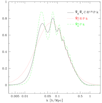
Figure 3: Integrands of the integrals appearing in equation (23) as functions of the wavevector for $\sigma_{8}=0.84$. Since the $k$-axis is logarithmic, the ordinate is multiplied by and extra power of $k$, so equal areas under a function correspond to equal contributions to an integral. Solid line shows the product $\widehat{W}_{\bf g}\widehat{W}_{\bf v}C{\cal R}^{1/2}Pk$, dotted – $\widehat{W}_{\bf v}^{2}{\cal R}Pk$, and dashed – $\widehat{W}_{\bf g}^{2}Pk$. Units of the ordinate axis are arbitrary.

4 Parameter estimation

We are now applying our formalism to the PSCz survey. As the value of $\sigma_{8}$ we adopt its WMAP’s estimate, $\sigma_{8}=0.84$ ($\pm 0.04$; Spergel et al. 2003). This specifies the coherence function and the ratio of the power spectrum of velocity to the power spectrum of gravity. Also, this provides a normalization for the power spectrum of density.

4.1 Parameter dependence of the model

As stated before, the likelihood of specific values of $\beta$ and $b$ is determined by the distribution (5). In this distribution, the observables are ${\bf g}$ and ${\bf v}$, or $g$, $v$, and the misalignment angle, $\psi$. Following S99, we adopt for them the following values: $g=933\;\hbox{km}\cdot\hbox{s}^{-1}$ (from the distribution of the PSCz galaxies up to $150\;h^{-1}\,\hbox{Mpc}$), $v=627\;\hbox{km}\cdot\hbox{s}^{-1}$ (inferred from the 4-year COBE data by Lineweaver et al. 1996), and $\psi=15^{\circ}$.

The theoretical quantities are $\sigma_{\bf g}$, $\sigma_{\bf v}$, and $r$. The variance of a single spatial component of measured gravity, $\sigma_{\bf g}^{2}$, is a sum of the cosmological component, $\sigma_{{\bf g},c}^{2}$, and errors, ${\epsilon}^{2}$. Since gravity here is inferred from a galaxian, rather than mass, density field, we have $\sigma_{{\bf g},c}^{2}=b^{2}s_{\bf g}^{2}$, where $s_{\bf g}^{2}$ is the variance of a single component of the true (i.e., mass-induced) gravity. From equation (17),

$$s_{\bf g}^{2}=\frac{1}{6\pi^{2}}\int_{0}^{\infty}\widehat{W}_{g}^{2}(k)P(k)dk\,.$$ (33)

The gravity errors are twofold: due to finite sampling of the galaxy density field, and due to the reconstruction of the galaxy density field in real space. Therefore, ${\epsilon}^{2}=(\sigma_{\rm SN}^{2}+\sigma_{\rm rec}^{2})/3$, where $\sigma_{\rm SN}^{2}$ and $\sigma_{\rm rec}^{2}$ are respectively the shot noise (or, sampling) variance and the reconstruction variance. (Both $\sigma_{\rm SN}^{2}$ and $\sigma_{\rm rec}^{2}$ are full, i.e., 3D, variances.) Estimated by S99 using mock catalogs, the cumulative shot noise at 150 $h^{-1}\,\hbox{Mpc}$ amounts to $\sigma_{\rm SN}=160$ $\hbox{km}\cdot\hbox{s}^{-1}$. An average reconstruction error in the differential contribution to the cumulative gravity, produced by a shell of matter $10$ $h^{-1}\,\hbox{Mpc}$ wide, is $15$ $\hbox{km}\cdot\hbox{s}^{-1}$. Since up to $150$ $h^{-1}\,\hbox{Mpc}$ there are $15$ such shells, we have $\sigma_{\rm rec}=\sqrt{15}\cdot 15$ $\hbox{km}\cdot\hbox{s}^{-1}$$=58$ $\hbox{km}\cdot\hbox{s}^{-1}$. To sum up,

$$\sigma_{\bf g}^{2}=b^{2}s_{\bf g}^{2}+\frac{\sigma_{\rm SN}^{2}+\sigma_{\rm rec}^{2}}{3}\,,$$ (34)

where

$$\sigma_{\rm SN}=160\;\hbox{km}\cdot\hbox{s}^{-1}\qquad{\rm and}\qquad\sigma_{\rm rec}=58\;\hbox{km}\cdot\hbox{s}^{-1}\,.$$ (35)

Errors in the measured velocity of the LG are negligible compared to those in the gravity. Equations (19) and (25) yield

$$\sigma_{\bf v}=\Omega_{m}^{0.6}s_{\bf v}\,,$$ (36)

where

$$s_{\bf v}^{2}=\frac{1}{6\pi^{2}}\int_{0}^{\infty}\widehat{W}_{v}^{2}(k)\tilde{\mathcal{R}}(k)P(k)dk\,.$$ (37)

Finally, errors in the estimate of the LG gravity do not affect the cross-correlation between the LG gravity and velocity, but increase the gravity variance. This has the effect of lowering the value of the cross-correlation coefficient. Specifically, from equations (25)–(26) and (34) we have

$$r=\rho\left(1+\frac{\sigma_{\rm SN}^{2}+\sigma_{\rm rec}^{2}}{3b^{2}s_{\bf g}^{2}}\right)^{-1/2},$$ (38)

where

$$\rho=\frac{\int_{0}^{\infty}\widehat{W}_{\bf g}(k)\widehat{W}_{\bf v}(k)\tilde{C}(k)\tilde{\cal R}^{1/2}(k)P(k)dk}{\left[\int_{0}^{\infty}\widehat{W}_{\bf g}^{2}(k)P(k)dk\right]^{1/2}\left[\int_{0}^{\infty}\widehat{W}_{\bf v}^{2}(k)\tilde{\cal R}(k)P(k)dk\right]^{1/2}}\,.$$ (39)

Thus, the likelihood depends explicitly on the parameters $b$ and $\Omega_{m}$. However, for reasons that will become evident later on, as the parameters to be estimated we choose $b$ and $\beta\equiv\Omega_{m}^{0.6}/b$. Since $\Omega_{m}^{0.6}=\beta b$, both $\sigma_{\bf g}$, $\sigma_{\bf v}$ and $r$ depend on $b$. On the other hand, only $\sigma_{\bf v}$ depends on $\beta$. This makes the derivation of the most likely value of $\beta$, given $b$, simple.

4.2 $\mn@boldsymbol{\beta}$ for known $\mn@boldsymbol{b}$

Using equations (5), (36), and the equality $\Omega_{m}^{0.6}=\beta b$, the logarithmic likelihood for $\beta$ takes on the form:

$$\ln\mathcal{L}(\beta)\!\!\!\! = \!\!\!\!-3\ln{2\pi}-3\ln[\sigma_{\bf g}bs_{\bf v}(1-r^{2})^{1/2}]-3\ln\beta$$ (40)

$$\!\!\!\!-\frac{1}{2(1-r^{2})}\left(\frac{g^{2}}{\sigma_{\bf g}^{2}}+\frac{v^{2}}{\beta^{2}b^{2}s_{\bf v}^{2}}-\frac{2r\mu gv}{\sigma_{\bf g}\beta bs_{\bf v}}\right).$$

To find its maximum, we calculate its partial derivative with respect to $\beta$, $\partial\ln\mathcal{L}/\partial\beta$, and equate it to zero. This yields the following equation:

$$3(1-r^{2})\beta^{2}+\frac{r\mu gv}{\sigma_{\bf g}bs_{\bf v}}\beta-\frac{v^{2}}{b^{2}s_{\bf v}^{2}}=0\,.$$ (41)

The LG gravity, inferred from the PSCz survey, is tightly coupled to its velocity, $1-r\ll 1$ and $1-\mu\ll 1$. (Specifically, $\mu=0.97$ and, for $\sigma_{8}$ around $0.8$, $r\simeq 0.93$.) At first approximation we can therefore assume $r=\mu=1$, hence

$$\beta_{1}=\frac{\sigma_{\bf g}}{bs_{\bf v}}\frac{v}{g}\,.$$ (42)

Using equation (34) we obtain finally

$$\beta_{1}=\frac{s_{\bf g}}{s_{\bf v}}\left(1+\frac{\sigma_{\rm SN}^{2}+\sigma_{\rm rec}^{2}}{3b^{2}s_{\bf g}^{2}}\right)^{1/2}\frac{v}{g}\,.$$ (43)

Thus, the best estimate of $\beta$ is not just the ratio of the LG velocity to its gravity: it is modified by nonlinear effects (which affect $s_{\bf v}$ through the function $\tilde{\cal R}$), different observational windows (which affect differently $s_{\bf g}$ and $s_{\bf v}$), and observational errors.

At next approximation, in equation (41) one could approximate $\beta^{2}$ by $\beta_{1}^{2}$. However, we have considered the case of known $b$ for illustrative purposes only and from now on we relax this assumption. In the next subsection we will analyze the joint likelihood for $\beta$ and $b$.

4.3 Joint likelihood for $\mn@boldsymbol{\beta}$ and $\mn@boldsymbol{b}$

Figure 4: Likelihood contours for the parameters $\beta$ and $b$, corresponding to the confidence levels of 68, 90 and 95%. The maximum of the likelihood function is denoted by a dot.

Figure 4 shows isocontours of the joint likelihood for $\beta$ and $b$, corresponding to the confidence levels of 68, 90 and 95%. The maximum of the likelihood is denoted by a dot. The corresponding values of $\beta$ and $b$ are respectively $0.66$ and $0.94$.

This figure illustrates the well-known problem of $\Omega_{m}$–bias degeneracy in cosmic density–velocity comparisons. A ‘common wisdom’ is that in these comparisons, only a degenerate combination of $\Omega_{m}$ and $b$, $\beta\equiv\Omega_{m}^{0.6}/b$, can be determined. Here this is not strictly true, since we have estimated the most likely values of both $\beta$ and $b$, so in principle we could solve for the best value of $\Omega_{m}$ alone. However, the isocontours of the likelihood are much more elongated along the $b$-axis than along the $\beta$-axis, making the resulting constraints on $\Omega_{m}$ much weaker than on $\beta$. In practice, therefore, from our analysis we cannot say much about $\Omega_{m}$ or bias separately. On the other hand, we can put fairly tight constraints on $\beta$.

To do this, one approach is not to use any external information on bias. In such a case, we marginalize over all possible values of $b$ (from zero to infinity). The resulting distribution for $\beta$ is shown in Figure 5 as a dashed line. The distribution is positively skewed, with lower limit on $\beta$ being stronger than the upper one. Specifically, we find that $\beta=0.64^{+0.24}_{-0.11}$ ($68$% confidence limits).

A better approach is to use the fact that the square root of the variance of the PSCz galaxy counts at 8 $h^{-1}\,\hbox{Mpc}$ is $\sigma_{8}^{PSCz}\simeq 0.75$ (Sutherland et al. 1999). Combined with WMAP’s estimate of $\sigma_{8}$, this yields for the bias of the PSCz galaxies the value about $0.9$. Therefore, we adopt here a conservative prior for the bias, namely that it is constrained to lie in the range $[0.7,1.1]$. These limits are marked in Figure 4 as dashed vertical lines. We marginalize the likelihood over the values of $b$ in this range. The resulting distribution for $\beta$ is shown in Figure 5 as a solid line. This distribution is also skewed and more peaked than the previous one. We obtain $\beta=0.66^{+0.21}_{-0.07}$ ($68$% confidence limits).

Figure 5: The marginal distribution for $\beta$. The result of marginalizing over all possible values of $b$ (from zero to infinity) is shown as a dashed line. The result of marginalizing over the values of $b$ in the range $[0.7,1.1]$ is shown as a solid line.

5 Summary and conclusions

We have performed a likelihood analysis of the LG acceleration, paying particular care to nonlinear effects. We have adopted a widely accepted assumption that the joint distribution of the LG acceleration and velocity is Gaussian. Then, two quantities describing nonlinear effects are relevant. The first one is the coherence function, or the cross-correlation coefficient of the Fourier components of the gravity and velocity fields. The second one is the ratio of the power spectrum of the velocity to the power spectrum of the gravity. Extending our previous work, we have studied both the coherence function and the ratio of the power spectra. Using numerical simulations we have performed fits to the two as functions of the wavevector and $\sigma_{8}$. Then, we have estimated the best values of the parameter $\beta$ and its errors. We have obtained $\beta=0.66^{+0.21}_{-0.07}$ at 68% confidence level.

The analysis of the LG acceleration performed by S92 and S99 was in a sense more sophisticated than ours. Both teams analyzed a differential growth of the gravity dipole in subsequent shells around the LG. Instead, here we used just one measurement of the total (integrated) gravity within a radius of $150\;h^{-1}\,\hbox{Mpc}$. Nevertheless, the errors on $\beta$ we have obtained are significantly smaller than those of S92 and S99. In particular, S99 obtained $\beta=0.70^{+0.35}_{-0.20}$ at $1\sigma$ confidence level. Comparing these errors to ours should be done with caution, because S99 considered the joint likelihood for $\beta$ and the index of the power spectrum, $\Gamma$. (To obtain a constraint on $\beta$, they marginalized the distribution over the values of $\Gamma$ allowed by the constraints on the Hubble constant.) Still, it is striking that while our best value of $\beta$ is close to theirs, our errors are significantly smaller. The reason is our careful modelling of nonlinear effects. In a previous paper (C02) we showed that the coherence function used by S99 greatly overestimates actual decoherence between nonlinear gravity and velocity. Tighter correlation between the LG gravity and velocity should result in a smaller random error of $\beta$; in the present work we have shown this to be indeed the case.

The second factor in the LG acceleration analysis, describing nonlinear effects, is the ratio of the power spectra of velocity to gravity. Unlike the coherence function, this quantity has not been accounted for previously. It affects the value of the correlation coefficient, hence the random error, to lesser extent than the CF. However, it does affect the most likely value of $\beta$, as can be easily noticed from illustrative equation (42) (via $s_{\bf v}$). Neglecting different nonlinear growth rates of the gravity and the velocity is equivalent to setting $\tilde{\cal R}=1$; we have checked that then the best value of $\beta$ is $0.62$. Therefore, a small discrepancy between our and S99’s most likely value of $\beta$ is not due to nonlinear effects.

Unlike ours, the analysis of S99 included also other constraints on the velocity field around the LG: its (small) shear, and the value of the bulk flow within $30\;h^{-1}\,\hbox{Mpc}$. This may have had an effect on the best value of $\beta$. Moreover, an approach with multiple windows should allow to further tighten the errors. It is therefore interesting to repeat the analysis of S99 exactly, but with proper treatment of nonlinear effects. We plan to do this in the future.

References

- [] Bernardeau F., Chodorowski M. J., Łokas E. L., Stompor R., Kudlicki A., 1999, MNRAS, 309, 543
- [] Bertschinger E., Dekel A., 1989, ApJ, 336, L5
- [] Bouchet F.R., Colombi S., Hivon E., Juszkiewicz R., 1995, A&A, 296, 575
- [] Catelan P., Moscardini L., 1994, ApJ, 436, 5
- [] Chodorowski M.J., Cieciela̧g P., 2002, MNRAS, 331, 133 (C02)
- [] Cieciela̧g P., Chodorowski M.J., Kiraga M., Strauss M.A., Kudlicki A., Bouchet F.R., 2003, MNRAS, 339, 641
- [] Courteau S., van den Bergh S., 1999, AJ, 118, 337
- [] Efstathiou G., Bond J.R., White S.D.M., 1992, MNRAS, 258, 1
- [] Juszkiewicz R., Vittorio N., Wyse R.F.G., 1990, ApJ, 349, 408
- [] Kofman L., Bertschinger E., Gelb J. M., Nusser A., Dekel A., 1994, ApJ, 420, 44
- [] Kudlicki A., Plewa T., Różyczka M., 1996, Acta A., 46, 297
- [] Kudlicki A., Chodorowski, M.J., Plewa T., Różyczka M., 2000, MNRAS, 316, 464
- [] Lahav O., Kaiser N., Hoffman Y., 1990, ApJ, 352, 448
- [] Lineweaver C.H., Tenorio L., Smoot G.F., Keegstra P., Banday A.J., Lubin P., 1996, ApJ, 470, L38
- [] Lynden-Bell D., Lahav O., Burstein D., 1989, MNRAS, 241, 325
- [] Mancinelli P. J., Yahil A., Ganon G., Dekel A., 1994, in Proceedings of the 9th IAP Astrophysics Meeting ‘Cosmic velocity fields’, ed. F. R. Bouchet and M. Lachièze-Rey, Gif-sur-Yvette: Editions Frontières, 215
- [] Meiksin A., Davis M., 1986, AJ, 91, 191
- [] Nusser A., Colberg J.M., 1998, MNRAS, 294, 457
- [] Pichon C., Bernardeau F., 1999, A&A, 343, 663
- [] Saunders W., et al., 2000, MNRAS, 317, 55
- [] Schmoldt I., et al., 1999, MNRAS, 304, 893 (S99)
- [] Scoccimarro R., Colombi S., Fry J.N., Frieman J.A., Hivon E., Melott A., 1998, ApJ, 496, 586
- [] Spergel D.N., et al., 2003, ApJS, 148, 175
- [] Strauss M.A., Davis M., 1988, ‘Large-Scale Motions in the Universe’, A Vatican Study Week, 255-274
- [] Strauss M.A., Yahil A., Davis M., Huchra J.P., Fisher K., 1992, ApJ, 397, 395 (S92)
- [] Sutherland W., et al., 1999, MNRAS, 308, 289
- [] Yahil A., Walker D., Rowan-Robinson M., 1986, ApJ, 301, L1
- [] Zaroubi S., 2002, Proceedings of the XIII Rencontres de Blois, ‘Frontiers of the Universe’, eds. L.M. Celnikier, et al., in press (astro-ph/0206052)