Improved Cosmological Constraints from Gravitational Lens Statistics

Abstract

We combine the Cosmic Lens All-Sky Survey (CLASS) with new Sloan Digital Sky Survey (SDSS) data on the local velocity dispersion distribution function of E/S0 galaxies, $\phi(\sigma)$, to derive lens statistics constraints on $\Omega_{\Lambda}$ and $\Omega_{m}$. Previous studies of this kind relied on a combination of the E/S0 galaxy luminosity function and the Faber-Jackson relation to characterize the lens galaxy population. However, ignoring dispersion in the Faber-Jackson relation leads to a biased estimate of $\phi(\sigma)$ and therefore biased and overconfident constraints on the cosmological parameters. The measured velocity dispersion function from a large sample of E/S0 galaxies provides a more reliable method for probing cosmology with strong lens statistics. Our new constraints are in good agreement with recent results from the redshift-magnitude relation of Type Ia supernovae. Adopting the traditional assumption that the E/S0 velocity function is constant in comoving units, we find a maximum likelihood estimate of $\Omega_{\Lambda}=0.74$–$0.78$ for a spatially flat unvierse (where the range reflects uncertainty in the number of E/S0 lenses in the CLASS sample), and a 95% confidence upper bound of $\Omega_{\Lambda}<0.86$. If $\phi(\sigma)$ instead evolves in accord with extended Press-Schechter theory, then the maximum likelihood estimate for $\Omega_{\Lambda}$ becomes $0.72$–$0.78$, with the 95% confidence upper bound $\Omega_{\Lambda}<0.89$. Even without assuming flatness, lensing provides independent confirmation of the evidence from Type Ia supernovae for a nonzero dark energy component in the universe.

1 Introduction

Gravitationally lensed quasars and radio sources offer important probes of cosmology and the structure of galaxies. The optical depth for lensing depends on the cosmological volume element out to moderately high redshift, so lens statistics can in principle provide valuable constraints on the cosmological constant or, more generally, the dark energy density and its equation of state (e.g., Fukugita, Futamase, & Kasai 1990; Fukugita & Turner 1991; Turner 1990; Krauss & White 1992; Maoz & Rix 1993; Kochanek 1996; Falco, Kochanek, & Muñoz 1998; Cooray & Huterer 1999; Waga & Miceli 1999; Waga & Frieman 2000; Sarbu, Rusin, & Ma 2001; Chae et al. 2002; Chae 2003).

However, the cosmological constraints derived from lens statistics have been controversial, mainly because of disagreements about the population of galaxies that can act as deflectors. Kochanek (1996; see also Falco et al. 1998; Kochanek et al. 1998) reported an upper bound of $\Omega_{\Lambda}<0.66$ at 95% confidence for a spatially flat universe ($\Omega_{m}+\Omega_{\Lambda}=1$), which is in marginal conflict with the current concordance cosmology, $\Omega_{\Lambda}=0.69\pm 0.04$ (Spergel et al. 2003). But subsequent studies have reached different conclusions (e.g., Chiba & Yoshii 1999; Waga & Miceli 1999; Cheng & Krauss 2000). For example, Chiba & Yoshii (1999) argued that optically-selected lenses actually favor $\Omega_{\Lambda}=0.7^{+0.1}_{-0.2}$ for a flat universe. At issue are uncertainties in several key ingredients of traditional lens statistics calculations: (i) the luminosity function for early-type (E/S0) galaxies, which dominate the lensing rate; (ii) the Faber-Jackson relation between luminosity and velocity dispersion for early-types; and (iii) the assumed density profiles of lens galaxies. The spread in derived cosmological constraints can be traced in large measure to uncertainties in the galaxy luminosity function: until recently, different redshift surveys yielded values for the local density of $L^{*}$ galaxies that differed by up to a factor of two. This source of uncertainty has now been largely eliminated by much larger galaxy redshift surveys, such as the Sloan Digital Sky Survey (SDSS) and the 2dF Galaxy Redshift Survey (2dFGRS) (Blanton et al. 2001, 2003; Yasuda et al. 2001; Norberg et al. 2002; Madgwick et al. 2002).

Even with the local galaxy luminosity function well determined, there is a crucial systematic uncertainty concerning changes to the deflector population with redshift. Many analyses of lens statistics have assumed that the velocity dispersion distribution function $\phi(\sigma)$ is independent of redshift (in comoving units). This is equivalent to saying that massive early-type galaxies have not undergone significant mergers since $z\sim 1$. Although galaxy counts appear to be consistent with this ‘no-evolution’ model in the concordance cosmology (Schade et al. 1999; Im et al. 2002), the observational uncertainties are still large and other possibilities cannot be ruled out. The problem for lens statistics is that evolution is degenerate with cosmology. Keeton (2002a) has argued that previous studies obtained strong limits on $\Omega_{\Lambda}$ only because they assumed that the evolution rate is independent of cosmology; dropping that assumption would make lens statistics largely insensitive to cosmology. One way to handle the degeneracy is to turn the problem around: adopt values for the cosmological parameters and attempt to constrain models of galaxy evolution (e.g., Ofek, Rix, & Maoz 2003; Chae & Mao 2003). Unfortunately, the small size of current samples precludes using more than toy models of evolution, and even then the uncertainties are too large to distinguish a simple no-evolution model from various theoretical predictions. It would still be nice to use lens statistics to probe cosmology while accounting for evolution using more than toy models.

The problems with the traditional approach to lens statistics have partly motivated an alternate approach, in which empirical calibrations of the deflector population are replaced with theoretical predictions from galaxy formation models (e.g., Narayan & White 1988; Kochanek 1995; Porciani & Madau 2000; Keeton & Madau 2001; Sarbu, Rusin, & Ma 2001; Li & Ostriker 2002). In these theory-based models, the deflector population is described by a dark matter halo mass function, $n(M,z)$, given by Press-Schechter theory (calibrated by N-body simulations, see Sheth & Tormen 1999; Sheth, Mo & Tormen 2001; Jenkins et al. 2001). The predicted mass function depends on cosmology, which causes the lensing optical depth to depend on $\Omega_{\Lambda}$ through the cosmological volume element, the density perturbation growth rate, and the merger histories of halos. Unlike in the traditional approach, here the optical depth decreases with increasing $\Omega_{\Lambda}$ — suggesting that the traditional lensing upper bound on $\Omega_{\Lambda}$ should be interpreted with caution. This ‘theoretical’ approach to lens statistics avoids some of the untested assumptions of the traditional approach and has the advantage of working directly with the deflector mass function rather than indirectly with a mass function inferred from the galaxy luminosity function. However, it faces challenges of its own, chiefly arising from theoretical uncertainties in relating dark matter halos to the properties of luminous galaxies. For example, galaxy formation models have difficulty reproducing the observed galaxy luminosity function and empirical galaxy dynamical scaling relations (e.g., White & Frenk 1991; Cole et al. 1994; Kauffmann et al. 1993, 1999; Somerville & Primack 1999; Benson et al. 2003). Since nearly all confirmed lens systems contain a luminous galaxy that plays a significant role in the lensing, the problems with galaxy formation models may cause concern about the theoretical approach to lens statistics.

The goal of this paper is to make two modifications to lens statistics calculations that enable improved cosmological constraints. The first modification involves using new data on the dynamical properties of galaxies. In standard models, the lensing optical depth is given by a weighted integral over the galaxy velocity dispersion distribution function, $\phi(\sigma)$ (Turner, Ostriker, & Gott 1984, also see §2.2). Previously, $\phi(\sigma)$ was inferred by combining the measured early-type galaxy luminosity function $\phi(L)$ with the empirical Faber-Jackson relation, $L(\sigma)$; hereafter, we call this the inferred velocity function. This estimator for $\phi(\sigma)$ has two disadvantages: (i) neglect of the scatter in the Faber-Jackson relation yields a biased and incorrectly confident estimate for $\phi(\sigma)$ (Kochanek 1994; Sheth et al. 2003); and (ii) use of the luminosity function complicates attempts to deal with galaxy evolution, since $\phi(L)$ is sensitive not only to dynamical galaxy number and mass evolution (which matter for lens statistics) but also to passive luminosity evolution (which does not affect lens statistics). To obviate these problems, it is preferable to use a direct measurement of the E/S0 velocity function. Fortunately, the SDSS recently provided this very measurement based on $\sim$30,000 E/S0 galaxies (Bernardi et al. 2003, 2004; Sheth et al. 2003). With these new data, we can eliminate an important source of bias and misestimated error in lens statistics calculations.

The second modification concerns galaxy evolution. To make contact with previous studies, we consider models in which $\phi(\sigma)$ is constant in comoving units. However, we also study models in which $\phi(\sigma)$ evolves according to a theoretical prescription. As just mentioned, the fact that $\phi(\sigma)$ evolves only due to occasional mergers means that it provides a more straightforward framework for incorporating evolution than the traditional route through the luminosity function. Newman & Davis (2000, 2002) present such a framework using extended Press-Schechter theory to compute the ratio of the velocity function at redshift $z$ to the local velocity function, $\phi(\sigma;z)/\phi(\sigma;0)$. While model predictions for the full velocity function $\phi(\sigma,z)$ are sensitive to the uncertain physics that causes discrepancies between galaxy formation models and observed galaxy populations, the prediction for the ratio $\phi(\sigma,z)/\phi(\sigma,0)$ isolates the evolution piece (Newman & Davis 2002) and is therefore much less sensitive to these uncertainties. By joining the theoretical evolution model to the empirical calibration of the local deflector population, we obtain a new hybrid approach to lens statistics that combines the best aspects (and omits the pitfalls) of the purely empirical or purely theoretical approaches used previously. In the end, we find that inclusion of the extended Press-Schechter model for evolution does not significantly change the central values of the cosmological parameters inferred from lensing statistics, though it does increase the associated uncertainties.

For the lens sample, we use the Cosmic Lens All Sky Survey (CLASS; Myers et al. 1995; Browne et al. 2003), which is the largest statistically complete survey for lenses. Chae et al. (2002) and Chae (2003) recently analyzed the CLASS sample using the traditional approach based on an inferred velocity function. We use the same sample but analyze it using our new approach to lens statistics. Other small technical differences between the analyses are discussed below.

The layout of the paper is as follows. In §2 we review the theoretical framework, including lensing by isothermal spheres, the formalism for lens statistics, and the model for redshift evolution of the deflector population. In §3 we discuss the required observational data, including the measured and inferred velocity dispersion distribution functions from the SDSS early-type galaxy sample, and the CLASS radio lens survey. In §4 we use a likelihood analysis of the lens data to derive constraints on cosmological parameters. We conclude in §5. In the Appendix we discuss the SDSS early-type galaxy selection process and its effect on our model inputs.

2 Theoretical Framework

2.1 The singular isothermal sphere lens

X-ray studies (e.g., Fabbiano 1989), dynamical analyses (e.g., Rix et al. 1997; Gerhard et al. 2001), and various lensing studies (e.g., Treu & Koopmans 2002; Koopmans & Treu 2003; Rusin, Kochanek, & Keeton 2003) all indicate that on the $\lesssim$10 kpc scales relevant for lensing, early-type galaxies can be modeled as singular isothermal spheres (SIS), with a density profile corresponding to a flat rotation curve,

$$\rho(r)=\frac{\sigma^{2}}{2\pi Gr^{2}}\ .$$ (1)

Here $\sigma$ is the velocity dispersion of the system, $r$ is the distance from the center of the galaxy, and we have assumed negligible core radii and ellipticities. While lens statistics are in principle sensitive to finite-density cores in lens galaxies (e.g., Chiba & Yoshii 1999; Cheng & Krauss 2000; Hinshaw & Krauss 1987), the elusiveness of ‘core images’ limits the sizes of cores to a level that is unimportant (Krauss & White 1992; Wallington & Narayan 1993; Rusin & Ma 2001; Keeton 2002b; Winn et al. 2004). Also, while departures from spherical symmetry are important in detailed models of individual lenses (e.g., Keeton, Kochanek, & Seljak 1997), they have remarkably little effect on lens statistics. Huterer, Keeton, & Ma (2004) show any biases from neglecting ellipticity and shear in lens statistics analyses are at the level of $\Delta\Omega_{M}<0.01$ and $\Delta\Omega_{\Lambda}<0.02$ (also see §4.5 below).

Consider light rays propagating from a source past a lens to the observer. For an SIS lens with velocity dispersion $\sigma$, the ray bending angle is $4\pi(\sigma/c)^{2}$, independent of impact parameter. Multiple imaging occurs if the physical impact parameter is less than $4\pi(\sigma/c)^{2}(D_{OL}D_{LS})/D_{OS}$, where $D_{OL}$, $D_{LS}$, and $D_{OS}$ are the angular diameter distances from observer to lens, lens to source, and observer to source, respectively. It is therefore useful to define the angular Einstein radius,

$$\theta_{E}=4\pi\left(\frac{\sigma}{c}\right)^{2}\frac{D_{LS}}{D_{OS}}~{},$$ (2)

such that sources located at angle $\theta_{S}<\theta_{E}$ from an SIS lens are multiply imaged. For a Friedmann-Robertson-Walker cosmology with cosmological constant $\Omega_{\Lambda}$, non-relativistic matter density $\Omega_{m}$, and curvature density $\Omega_{k}=1-\Omega_{\Lambda}-\Omega_{m}$, the angular diameter distance can be written

$$D_{xy}=\frac{r_{xy}}{1+z_{y}}=\frac{c}{H_{0}}\frac{S_{k}(\chi_{xy})}{1+z_{y}}$$ (3)

where $r_{xy}$ is the transverse comoving distance, $H_{0}$ is the Hubble constant,

$$S_{k}(\chi_{xy})=\left\{\begin{array}[]{ll}\frac{1}{\sqrt{|\Omega_{k}|}}\ \sin(\sqrt{|\Omega_{k}|}\ \chi_{xy})&\mbox{if $\Omega_{k}<0$}\\ \frac{1}{\sqrt{\Omega_{k}}}\ \sinh(\sqrt{\Omega_{k}}\ \chi_{xy})&\mbox{if $\Omega_{k}>0$}\\ \chi_{xy}&\mbox{if $\Omega_{k}=0$}\end{array}\right.\mbox{,}$$ (4)

and

$$\chi_{xy}=\int_{z_{x}}^{z_{y}}dz\ \left[\Omega_{k}(1+z)^{2}+\Omega_{\Lambda}+\Omega_{m}(1+z)^{3}\right]^{-1/2}\ .$$ (5)

Here and throughout, we specialize to the case where the dark energy is identical to a cosmological constant; the generalization to a different dark energy equation of state is straightforward (Waga & Miceli 1999; Cooray & Huterer 1999).

A source at angular separation $\theta_{S}<\theta_{E}$ from an SIS lens yields two images on opposite sides of the lens at angular positions

$$\theta_{\pm}=\theta_{E}\pm\theta_{S}\ ,$$ (6)

which have magnifications

$$\mu_{\pm}=\frac{\theta_{E}\pm\theta_{S}}{\theta_{S}}~{}.$$ (7)

The image at $\theta_{-}$ has $\mu_{-}<0$ indicating that this image is parity reversed. The angular separation between the images is $\Delta\theta=2\theta_{E}$, independent of the source position. The total magnification of the two images is

$$\mu_{tot}=\frac{2\theta_{E}}{\theta_{S}}\ ,$$ (8)

and the bright-to-faint image flux ratio is

$$f=\frac{\theta_{E}+\theta_{S}}{\theta_{E}-\theta_{S}}\ .$$ (9)

In general lens surveys have a limited dynamic range, so a lens will be identified only if the flux ratio is less than some value; the CLASS survey included an explicit cut at $f_{max}=10$ (see §3.2). Thus only sources with $\theta_{S}<\theta_{max}<\theta_{E}$ will lead to detectable lenses, where

$$\frac{\theta_{max}}{\theta_{E}}=\frac{f_{max}-1}{f_{max}+1}\ .$$ (10)

2.2 Lens statistics

The optical depth for lensing is obtained by summing the cross sections for all deflectors between observer and source. Since the SIS cross section depends only on the lens velocity dispersion and cosmological distances, the property of the deflector population that is directly relevant is the velocity function, $\phi(\sigma)$. The optical depth for lensing can be written as an integral over $\phi(\sigma)$ (see, e.g., Turner, Ostriker, & Gott 1984),

$$\tau(z_{S},\Omega_{m},\Omega_{\Lambda})=\frac{1}{4\pi}\int_{0}^{z_{S}}{dV}\int_{0}^{\infty}{d\sigma\ \phi(\sigma;z_{L})}\ A(\sigma,\Omega_{m},\Omega_{\Lambda},z_{L},z_{S})B(S_{\nu})~{},$$ (11)

where $z_{S}$ and $z_{L}$ are the source and lens redshifts, $A$ is the cross section for multiple imaging, $B$ is the magnification bias (defined below), and the differential comoving volume element is

$$dV=4\pi r_{OL}^{2}\,\frac{dr_{OL}}{dz_{L}}d\,z_{L}~{}.$$ (12)

For an SIS lens, the angular separation between the two images is always twice the Einstein radius, so we can replace the integral over velocity dispersion with one over image separation.

Magnification bias accounts for the fact that intrinsically faint sources can appear in a flux-limited survey by virtue of the lensing magnification. The product of the cross section $A$ and the magnification bias $B$ can be written as

$$A(\sigma,\Omega_{m},\Omega_{\Lambda},z_{L},z_{S})B(S_{\nu})=2\pi\int^{\theta_{max}}_{0}d\theta_{S}\ \theta_{S}\ \frac{N(>\!S_{0}/\mu_{tot})}{N(>\!S_{0})}\ ,$$ (13)

where $N(>\!S)$ is the number of sources brighter than flux $S$, $S_{0}$ is the flux limit of the survey, and it is appropriate to use the total magnification $\mu_{tot}$ when the sources in the original flux-limited catalog are unresolved. If the source counts can be modeled as a power law, $dN/dS\propto S^{-\eta}$ (a good approximation for CLASS sources; Chae et al. 2002), then eqn. 13 can be evaluated to be

$$AB=\pi\theta_{E}^{2}\times\frac{2^{\eta}}{3-\eta}\left(\frac{f_{max}-1}{f_{max}+1}\right)^{3-\eta},$$ (14)

for an SIS lens population. Note that, absent a flux ratio cut, the cross section for an SIS lens would just be $A=\pi\theta_{E}^{2}$. It is convenient to define a combined correction factor ${\tilde{B}}$ that accounts for both magnification bias and the flux ratio limit of the lens survey,

$${\tilde{B}}(\eta,f_{max})\equiv\frac{AB}{\pi\theta_{E}^{2}}~{}.$$ (15)

From the total optical depth $\tau$ we can determine several interesting statistical distributions. $d\tau/d\Delta\theta$ describes the distribution of image separations, $d\tau/dz_{L}$ gives the redshift distribution of lens galaxies, and $d^{2}\tau/dz_{L}d\Delta\theta$ gives the joint distribution for both the lens galaxy redshift $z_{L}$ and the image separation $\Delta\theta$. All three of these distributions, together with the total optical depth, are used in the likelihood analysis of the CLASS survey (see §4).

2.3 A model for redshift evolution of the lens population

Many previous studies of lens statistics have assumed the velocity function $\phi(\sigma)$ to be constant in comoving units. This no-evolution assumption is usually justified by appealing to results from galaxy number counts (Im et al. 2002; Schade et al. 1999) and the redshift distribution of lens galaxies (Ofek, Rix, & Maoz 2003), which are consistent with the hypothesis that the early-type population evolves only through passive luminosity evolution. However, the observational status of early-type evolution has been controversial (Lin et al. 1999; Kauffmann, Charlot, & White 1996; Totani & Yoshii 1998; Fried et al. 2001), and the observational uncertainties are large enough that dynamical number or mass evolution in the early-type galaxy population cannot be ruled out.

Evolution of $\phi(\sigma)$ in amplitude or shape could substantially impact cosmological constraints from lens statistics. In order to gauge these effects, we adopt an evolution model based on theoretical galaxy formation models. Following Newman & Davis (2000, 2002), we use extended Press-Schechter theory to compute the ratio of the velocity dispersion function at two epochs, $\phi(\sigma;z)/\phi(\sigma;0)$, as a function of cosmological parameters. This ratio can be combined with the measured local velocity dispersion function $\phi(\sigma;0)$ to estimate $\phi(\sigma;z)$ at any epoch. As discussed in the Introduction, this estimate represents a hybrid approach to lens statistics that combines a careful measurement of the local velocity function with a simple but robust theoretical prediction for evolution.

N-body simulations of structure formation in cold dark matter models (e.g., Jenkins et al. 2001) indicate that the halo mass function at epoch $z$ is well fit by the modified Press-Schechter form introduced by Sheth & Tormen (1999),

$$n(M;z)={\bar{\rho}\over M}\,{d\ln\nu\over dM}\,A(p)\left[1+(q\nu)^{-p}\right]\left({q\nu\over 2\pi}\right)^{1/2}\,\exp(-q\nu/2)\,,$$ (16)

where $\bar{\rho}$ is the mean density, $\nu(z)=\delta_{c}^{2}/\sigma^{2}_{\delta}(M,z)$, $\delta_{c}=1.686$ is the extrapolated linear overdensity of a spherical top hat perturbation at the time it collapses, $\sigma^{2}_{\delta}(M,z)$ is the variance of the density field at epoch $z$ in linear perturbation theory, smoothed with a top hat filter of radius $R=(3M/4\pi\bar{\rho})^{1/3}$, and the fitting parameters have values $p=0.3$, $A(p)=0.3222$, and $q=0.75$. The smoothed variance is given in terms of the present linear density power spectrum $P(k)$ by

$$\sigma^{2}_{\delta}(M,z)={D^{2}(z)\over 2\pi^{2}}\int_{0}^{\infty}k^{2}\,P(k)\,W^{2}(k;M)\,dk\,,$$ (17)

where $W(k;M)$ is the Fourier transform of the top hat window function of radius $R(M)$. The linear growth factor is given by $D(z)=I(z)/I(0)$, where

$$I(z)=\int_{z}^{\infty}{{1+z}\over E(z)^{3}}\,dz\,,$$ (18)

and $E(z)=H(z)/H_{0}=\left[\Omega_{m}(1+z)^{3}+\Omega_{\Lambda}+\Omega_{k}(1+z)^{2}\right]^{1/2}$.

To convert the mass function into a velocity function, we must take into account the formation epoch of halos: those that form earlier will be more concentrated and have higher velocity dispersion for fixed mass. Following a simplified version of the procedure in Newman & Davis (2000), we use the results of Lacey & Cole (1994) to estimate the mean formation redshift $z_{f}$ for a halo of mass $M$ observed at redshift $z$. Lacey & Cole (1994) define a scaled variable

$${\tilde{\omega}_{f}}=\delta_{c}\ {{D^{-1}(z_{f})-D^{-1}(z)}\over[\sigma^{2}_{\delta}(M/2,0)-\sigma^{2}_{\delta}(M,0)]^{1/2}}\ ,$$ (19)

and the distribution of formation redshifts is given implicitly by the probability distribution $dp/d{\tilde{\omega}_{f}}$. N-body simulations indicate that $dp/d{\tilde{\omega}_{f}}$ is nearly independent of halo mass and of the power spectrum shape (Lacey & Cole 1994); following their Figure 12, we approximate this distribution by a delta function at $\langle{\tilde{\omega}_{f}}\rangle=0.9$. While this effectively ignores the dispersion of formation epoch, we have checked that this approximation does not significantly affect the estimate of $\phi(\sigma;z)/\phi(\sigma;0)$ over the range of interest.

Figure 1: The ratio of the velocity function of halos at $z=1$ to that at $z=0$. The points show results from a high-resolution N-body simulation by A. Kravtsov (private communication), and the dashed curve shows results from the extended Press-Schechter theory for the same cosmological parameters. The solid curve shows the extended Press-Schechter prediction for the best-fit flat cosmology from lens statistics for the CLASS sample (see §4), keeping $h=0.7$ and $\sigma_{8}=0.9$ fixed.

Solving eqn. 19 for $z_{f}$, and modeling each halo as an SIS, we can infer the velocity dispersion (Newman & Davis 2000; Bryan & Norman 1997),

$$\sigma(M,z)=92.3\,\Delta_{\rm vir}(z_{f})^{1/6}\,E(z_{f})^{1/3}\,\left({M\over 10^{13}\,h^{-1}M_{\odot}}\right)^{1/3}\ {{\rm km}\over{\rm sec}}\ ,$$ (20)

where (Bryan & Norman 1997)

$$\Delta_{\rm vir}(z)=18\pi^{2}+60[\Omega(z)-1]-32[\Omega(z)-1]^{2}~{},$$ (21)

and

$$\Omega(z)={\Omega_{m}(1+z)^{3}\over E^{2}(z)}~{}.$$ (22)

Combining eqn. 20 with eqn. 16 yields the velocity function $\phi(\sigma;z)$. Figure 1 shows the ratio $\phi(\sigma;1)/\phi(\sigma;0)$ versus $\sigma$ for several sample cases. In general, $\phi(\sigma;z)$ grows with redshift for $\sigma$ less than a few hundred km/sec, and the growth is strongly dependent on cosmological parameters. We have checked that the model agrees well with high-resolution N-body simulations (A. Kravstov, private communication; see Fig. 1).

In Fig. 1, we have also included the evolution ratio that results from the parameterized evolution by Chae & Mao (2003). By comparing our model with Chae & Mao (2003) in Fig. 1, one might wonder if our dynamical evolution model is missing some evolution at high $\sigma$. However, the Chae & Mao (2003) model actually captures both dynamical evolution and passive luminosity evolution, whereas our model neatly isolates the dynamical evolution.

We caution that the Press-Schechter model describes the behavior of dark halos, and we are assuming that it applies to luminous, early-type galaxies. While this ignores subtleties associated with baryonic infall and luminous galaxy formation, the N-body simulations shown above do have sufficiently high resolution to resolve galactic-scale subhalos, and they are included in the results for $\phi(\sigma)$. Moreover, SPH and semi-analytic models indicate that moderately massive halos contain a luminous, central galaxy. To the extent that the measured velocity dispersions of early-type galaxies provide good estimates of the velocity dispersions of the sub-halos they occupy (see §3.1.1), this model should provide a reasonable approximation to the evolution of $\phi(\sigma)$ for early-type galaxies. In addition, since we are computing a ratio (which is generally less than 2 for the redshifts and velocity dispersions of interest for lensing), it should not be extremely sensitive to these subtle effects (for details, see Newman & Davis 2002).

3 Observational Inputs

3.1 The deflector population

We follow the traditional approach to lens statistics and assume that all lenses are associated with optically luminous galaxies and calibrate the deflector population empirically. Furthermore, we focus on early-type galaxies. Although late-type galaxies are more abundant than early-types, they tend to have lower masses and hence to contribute no more than 10–20% of the lensing optical depth. This is a standard prediction of lens statistics models (Turner, Ostriker, & Gott 1984; Fukugita & Turner 1991; Maoz & Rix 1993) that has been borne out by the data (e.g., Fassnacht & Cohen 1998; Keeton, Kochanek, & Falco 1998; Kochanek et al. 2000; Lubin et al. 2000). We could attempt to model both the early- and late-type deflector populations in order to compute the total lensing optical depth and compare to the observed number of lenses produced by early- and late-type galaxies (as done by Chae et al. 2002; Chae 2003). However, we believe it is simpler and more instructive to separate the galaxy types, to compute the optical depth due to early-type galaxies alone, and to compare that to the number of lenses produced by early-type galaxies. This allows us to avoid dealing with uncertainties in the description of the late-type galaxy population.

In the following sections we describe two models for the distribution of the early-type deflectors. First, we use a direct measurement of the early-type velocity dispersion function. We then specify an inferred velocity dispersion function using the early-type luminosity function transformed by the mean Faber-Jackson relation in order to make contact with and compare to previous studies of this type.

3.1.1 The measured velocity function

We calibrate the E/S0 deflector population using a sample of $\sim$30,000 early-type galaxies at redshifts $0.01\leq z\leq 0.3$ selected from the SDSS database following Bernardi et al. (2003, 2004). A detailed description of the selection procedure is given in the Appendix. Briefly, the selection is based on both morphological and spectral criteria: the sample is restricted to galaxies with de Vaucouleurs surface brightness profiles that lack strong emission lines, for which measurements of the velocity dispersion are available.

The SDSS data reduction pipelines only measure velocity dispersions for galaxies with spectra of sufficiently high signal to noise to ensure accurate measurement. In addition, the resolution of the SDSS spectrographs prevents accurate estimates of dispersions smaller than $\sigma=70$ km/sec (Bernardi et al. 2003). Since this cutoff corresponds to a typical lens image separation of $\Delta\theta\lesssim 0\farcs 14$, well below the $0\farcs 3$ resolution limit of the CLASS survey, it has a negligible effect on our analysis. The Appendix describes various tests of the selection procedure which suggest that the sample does not miss more than, and probably much less than, 30% of the early-type population. We therefore disagree with the claim by Chae (2003) that the Bernardi et al. sample is too restrictive to be representative of the early-type population, at least as regards the velocity function relevant for lensing.

The SDSS E/S0 sample size has increased from the $\sim$9000 used by Bernardi et al. (2003) to $\sim$30,000 used by Bernardi et al. (2004), purely because a larger fraction of the sky has now been observed. There are small differences in the data that arise from modifications to the SDSS data reduction pipeline; see Bernardi et al. (2004) for details. Briefly, the new model magnitudes (which are used to fit the $L(\sigma)$ relation) are fainter by $\sim$0.12 mag, and the half-light radii $\theta_{\rm eff}$ are smaller by $\sim$10%. The change in size causes a small change in the velocity dispersions: while the measured dispersions are the same, the aperture correction from the SDSS fiber radius ($\theta_{\rm fiber}=1\farcs 5$) to a uniform physical radius (conventionally taken to be $\theta_{\rm eff}/8$) has changed. (It is the aperture-corrected ‘central’ velocity dispersions that we need, because these are very nearly equal to the dark matter velocity dispersions needed for the lensing calculations; see Franx 1993; Kochanek 1993, 1994; Treu & Koopmans 2004). Observed velocity dispersion profiles typically fall as weak power laws, so the correction has the form $\sigma_{\rm ap-cor}=\sigma_{\rm fiber}(8\theta_{\rm fiber}/\theta_{\rm eff})^{0.04}$, and the decrease in $\theta_{\rm eff}$ leads to a slight increase in the aperture-corrected velocity dispersions. These revisions to the SDSS photometry have affected the luminosity and velocity functions of the E/S0 sample as well as the slope of the $\sigma(L)$ relation.

Figure 2: The data points show the measured velocity function (MVF) for the sample of $\sim$30,000 early-type galaxies in the SDSS. The heavy and light solid curves show the best Schechter-like fits to the SDSS measured (MVF) and inferred (IVF) velocity functions, respectively. For comparison, the dashed curve shows the IVF for the SSRS2 early-type galaxy sample (Marzke et al. 1998), after the normalization correction applied by Chae (2003).

Sheth et al. (2003) use the aperture-corrected dispersions to compute the velocity function, which is shown by the points in Figure 2 (for the revised sample from Bernardi et al. 2004). The function can be modeled as a modified Schechter function (Schechter 1976) of the form

$$\phi(\sigma)\,d\sigma=\phi_{*}\left(\frac{\sigma}{\sigma_{*}}\right)^{\alpha}\ \exp\left[-\left(\frac{\sigma}{\sigma_{*}}\right)^{\beta}\right]\ \frac{\beta}{\Gamma(\alpha/\beta)}\ \frac{d\sigma}{\sigma}\ ,$$ (23)

where $\phi_{*}$ is the integrated number density of galaxies, $\sigma_{*}$ is a characteristic velocity dispersion, $\alpha$ is the low-velocity power-law index, and $\beta$ is the high-velocity exponential cutoff index of the distribution. The best-fit parameter values are

$$(\phi_{*},\sigma_{*},\alpha,\beta)_{MVF}=((1.4\pm 0.1)\times 10^{-3}\ {h_{70}^{3}\rm Mpc}^{-3},\ 88.8\pm 17.7\ {\rm km/sec},\ 6.5\pm 1.0,\ 1.93\pm 0.22)\ ,$$ (24)

where the Hubble parameter $H_{0}=70\,h_{70}$ km/sec/Mpc. The curve in Figure 2 shows this fit. Possible evolution in the velocity function can be treated as redshift dependence in the parameters $\phi_{*}$, $\sigma_{*}$, $\alpha$, and/or $\beta$.

The new, larger sample of $\sim$30,000 early-type galaxies in the SDSS contains a small surplus of galaxies with velocity dispersions $\geq$450 km/sec that is not fit by the Schechter function (see Fig. 2). Although massive, such galaxies are sufficently rare that they contribute only $\sim$0.2% of the lensing optical depth, so we have not attempted to modify the MVF fit to include them.

Using the Schechter-like fit for the velocity function, the optical depth becomes (see eqn. 11)

$$\tau(z_{S},\Omega_{m},\Omega_{\Lambda})=\int_{0}^{z_{S}}\tau_{*}(z_{L})\left(\frac{r_{OL}r_{LS}}{r_{OS}}\right)^{2}\frac{dr_{OL}}{dz_{L}}\ dz_{L}\ {\tilde{B}}(\eta,f_{max})$$ (25)

where

$$\tau_{*}(z)=16\pi^{3}\,\phi_{*}(z)\left[\frac{\sigma_{*}(z)}{c}\right]^{4}\ \frac{\Gamma\left[\frac{\alpha(z)+4}{\beta(z)}\right]}{\Gamma\left[\frac{\alpha(z)}{\beta(z)}\right]}\ .$$ (26)

If there is no evolution in $\phi(\sigma)$ then $\tau_{*}$ is just a constant that can be pulled out of the integral in eqn. 25. For a flat cosmology, the redshift integral in eqn. 25 can be evaluated analytically; in this no-evolution flat case, the optical depth is $\tau=\tau_{*}\,{\tilde{B}}\,(c/H_{0})^{3}\,r_{OS}^{3}/{30}$. This simple example illustrates how lens statistics probe the volume of the universe out to the redshifts of the sources.

3.1.2 The inferred velocity function

As discussed in the Introduction, previous analyses of lens statistics usually obtained an estimate of the velocity function by taking an observed galaxy luminosity function and transforming it using the Faber-Jackson relation; we refer to this estimate as the inferred velocity function, or IVF. Generally, the luminosity function is modeled as a Schechter function,

$$\phi(L)\,dL={\tilde{\phi}}_{*}\left(\frac{L}{L_{*}}\right)^{\tilde{\alpha}}\exp\left[-\left(\frac{L}{L_{*}}\right)\right]\ \frac{dL}{L_{*}}\ ,$$ (27)

where the parameters are the comoving number density of galaxies ${\tilde{\phi}}_{*,LF}$, the characteristic luminosity $L_{*}$ (or corresponding absolute magnitude $M^{*}$), and the faint-end slope $\tilde{\alpha}_{LF}$. With a Faber-Jackson relation of the form $L/L_{*}=(\sigma/\sigma_{*})^{\gamma}$, the IVF becomes

$$\phi(\sigma)\,d\sigma={\tilde{\phi}}_{*}\left(\frac{\sigma}{\sigma_{*}}\right)^{\gamma({\tilde{\alpha}}+1)-1}\ \exp\left[-\left(\frac{\sigma}{\sigma_{*}}\right)^{\gamma}\right]\ \gamma\ \frac{d\sigma}{\sigma_{*}}\ .$$ (28)

The coefficient of the optical depth, $\tau_{*}$, for this distribution differs slightly from the form of eqn. 26:

$$\tau_{*}=16\pi^{3}\,{\tilde{\phi}_{*}}\left(\frac{\sigma_{*}}{c}\right)^{4}\ \Gamma\left[1+{\tilde{\alpha}}+\frac{4}{\gamma}\right]\ .$$ (29)

With this change, the optical depth has the same form as eqn. 25.

We must consider how evolution in the deflector population could affect the velocity function. Dynamical evolution due to mergers would change both the luminosity function and the velocity function. Passive luminosity evolution (due to aging stellar populations) would affect the luminosity function but not the velocity function, at least for simple models. If galaxies of different luminosities have the same passive evolution rate, then $L$ depends on redshift but $L/L_{*}$ does not. Conceptually, the changes in the luminosity function are offset by corresponding changes in the Faber-Jackson relation such that the IVF remains constant. This makes sense, because the velocity function describes the dynamical properties of galaxies so any evolution that leaves the dynamics unchanged must also leave the velocity function unchanged. We focus on a non-evolving velocity function when using the IVF.

Chae (2003) and Chae et al. (2002) recently analyzed the statistics of CLASS lenses using an IVF based on the Second Southern Sky Redshift Survey (SSRS2). SSRS2 is a relatively shallow ($z\leq 0.05$), bright ($m_{B}\leq 15.5$) survey that contained only 5404 galaxies but allowed visual classification of the morphological types (Marzke et al. 1998), yielding 1595 early-type galaxies. With this small sample, the normalization is sure to suffer biases from large-scale inhomogeneities; to compensate, Chae corrected the normalization using the total luminosity function normalization scaled by the fraction of early-types measured in other, larger surveys. The Schechter luminosity function parameters for the early-type galaxy sample, as reported by Chae (2003), are

$$({\tilde{\phi}}_{*},M^{*}_{0}-5\ log_{10}\ h_{70},{\tilde{\alpha}})_{LF,\ SSRS2}=(2.2\times 10^{-3}\ {h_{70}^{3}\rm Mpc}^{-3},-20.40,\ -1.0)\ .$$ (30)

Chae (2003) and Chae et al. (2002) fixed the Faber-Jackson index at $\gamma=4$. Rather than using external constraints on $\sigma_{*}$, they chose to calibrate this parameter as part of their likelihood analysis of CLASS lenses. In effect, $\sigma_{*}$ was determined by the distribution of lens image separations. The resulting best-fit IVF parameters for SSRS2 are

$$({\tilde{\phi}}_{*},\sigma_{*},\gamma{\tilde{\alpha}}+\gamma-1,\gamma)_{IVF,\ SSRS2}=(2.2\times 10^{-3}\ {h_{70}^{3}\rm Mpc}^{-3},\ 198\ {\rm km/sec},\ -1.0,\ 4.0)\ .$$ (31)

This fit is shown as the dashed line in Figure 2. There are two possible causes for concern in the use of the lens image separation distribution for an internal calibration of $\sigma_{*}$. First, this approach introduces Poisson errors associated with the small lens sample. Second, it may introduce systematic biases if the small number of lens galaxies in the sample are not representative of massive early-type galaxies. Use of the velocity dispersion function measured directly from a large sample avoids both of these problems.

We can also obtain an IVF for the SDSS early-type galaxy sample. The error bars in Figure 3 show the measured luminosity function for the revised SDSS sample from Bernardi et al. (2004). The dashed line shows a Gaussian fit to the data reported by Bernardi et al. (2003), but shifted faintwards by 0.125 mag and downwards to $\phi_{*}=0.001$, as required by the new data reductions. We have refit the sample with a modified Schechter function (eqn. 23), finding best-fit parameters

$$(\phi_{*},M^{*}_{r},\alpha,\beta)_{LF,SDSS}=(1.4\times 10^{-3}\ {h_{70}^{3}\rm Mpc}^{-3},\ -16.46-0.85z,\ 2.53,\ 0.43)\ .$$ (32)

The solid curve in Figure 3 show this fit. Compared to the Gaussian fit, the Schechter fit does a better job at both the faint end (which is why its normalization $\phi_{*}$ is slightly larger) and the bright end, so we focus on it.

Figure 3: The SDSS E/S0 luminosity function. The points show the data from the sample of $\sim$30,000 galaxies given by Bernardi et al. (2004). The dashed line shows the Gaussian fit reported by Bernardi et al. (2003), with $M^{*}$ increased by 0.125 and the normalization reduced to $\phi_{*}=0.001$ to adjust to the updated photometry (see Bernardi et al. 2004). The solid line shows our Schechter fit.

The SDSS sample also provides a direct calibration of the $L(\sigma)$ (Faber-Jackson) relation. With the sample from Bernardi et al. (2004), the mean inverse relation is (see Fig. 14 in the Appendix)

$$\langle\log_{10}(\sigma/{\rm km~{}sec}^{-1})\mid M_{r}\rangle=2.2-0.091(M_{r}+20.79+0.85z)\,,$$ (33)

which corresponds to a Faber-Jackson index $\gamma=4.4$. Thus, the SDSS IVF is described by the parameters

$$(\phi_{*},\sigma_{*},\alpha,\beta)_{IVF,SDSS}=(1.4\times 10^{-3}\ {h_{70}^{3}\rm Mpc}^{-3},\ 64.0\ {\rm km/sec},\ 11.13,\ 1.89)\ ,$$ (34)

which is also shown in Figure 2.

Clearly both the SSRS2 and SDSS IVFs differ systematically from the SDSS MVF. Sheth et al. (2003) showed that the difference between the SDSS IVF and MVF is due to the fact that the IVF ignores the considerable dispersion in the $L(\sigma)$ relation. They found that the RMS scatter around the mean inverse relation (eqn. 33) is

$${\rm rms}(\log_{10}(\sigma/{\rm km~{}sec}^{-1})\mid M_{r})=0.79\ [1+0.17\ (M_{r}+21.025+0.85z)]\ .$$ (35)

(This result holds for both the original and revised SDSS samples.) The scatter broadens the velocity function and, in particular, raises the tail to high $\sigma$ without changing the mean (also see Kochanek 1994). The impact on lens statistics is apparent when we examine the differential ‘lensing efficiency’ (LE), or the contribution to the lensing optical depth from each $\sigma$ bin (see eqn. 26):

$$LE\equiv\phi(\sigma)\,\sigma^{4}\propto\frac{d\tau}{d\sigma}\ .$$ (36)

Figure 4 shows the lensing efficiency for the SSRS2 IVF, the SDSS IVF, and the SDSS MVF. The IVF substantially underestimates the abundance of massive early-type galaxies and hence the total optical depth. This effect leads directly to a lensing estimate for $\Omega_{\Lambda}$ that is biased high (see §5). The effect can be seen quantitatively by comparing $\tau_{*}=6.92\times 10^{-3}$ for the SDSS MVF, versus $\tau_{*}=5.79\times 10^{-3}$ for the SDSS IVF.

Figure 4: A comparison of the lensing efficiency, $LE\equiv\phi(\sigma)\,\sigma^{4}$, for the measured and inferred velocity functions from the SDSS early-type galaxy sample, and for the inferred velocity function from the SSRS2 early-type galaxy sample.

3.2 Radio source lens survey: CLASS

Survey	Name	$z_{L}$	$z_{S}$	$\Delta\theta$	Lens	Reference
JVAS	B0218+357	0.68	0.96	0.33	S	Patnaik et al. (1993)
CLASS	B0445+123	0.56	—	1.33	?	Argo et al. (2003)
CLASS	B0631+519	—	—	1.16	?	Browne et al. (2003)
CLASS	B0712+472	0.41	1.34	1.27	E	Jackson et al. (1998)
CLASS	B0850+054	0.59	—	0.68	?	Biggs et al. (2003)
CLASS	B1152+199	0.44	1.01	1.56	?	Myers et al. (1999)
CLASS	B1359+154	—	3.21	1.65	?, m	Myers et al. (1999)
JVAS	B1422+231	0.34	3.62	1.28	E	Patnaik et al. (1992b)
CLASS	B1608+656	0.64	1.39	2.08	E, m	Myers et al. (1995)
CLASS	B1933+503	0.76	2.62	1.17	E	Sykes et al. (1998)
CLASS	B2045+265	0.87	1.28	1.86	?	Fassnacht et al. (1999)
JVAS	B2114+022	0.32/0.59	—	2.57	E, m	Augusto et al. (2002)
CLASS	B2319+051	0.62/0.59	—	1.36	E	Rusin et al. (2001b)

Table 1: Data for the 13 Lenses in the CLASS statistical sample of 8958 objects (adapted from Browne et al. (2003), Chae (2003), and Davis, Huterer, & Krauss (2003)). “Lens” stands for the morphology of the lens galaxy: spiral (S), elliptical (E), or unknown (?); three lenses contain multiple galaxies (m).

While some 80 multiply imaged quasars and radio sources have been discovered, a statistical analysis requires a sample from a survey that is complete and has well-characterized, homogeneous selection criteria. The largest such sample comes from the radio Cosmic Lens All-Sky Survey (CLASS; Browne et al. 2003; Myers et al. 2003), an extension of the earlier Jodrell Bank/Very Large Array Astrometric Survey (JVAS; Patnaik et al. 1992a; King et al. 1999). About 16,000 sources have been imaged by JVAS/CLASS, with 22 confirmed lenses. Of these, a subset of 8958 sources with 13 lenses forms a well-defined subsample suitable for statistical analysis (Browne et al. 2003). The properties of these lenses are summarized in Table 1. Of the 13 lenses, 8 have measured source redshifts, 11 have measured lens redshifts, and 7 have both (Chae et al. 2002).

Radio lens surveys (Quast & Helbig 1999; Helbig et al. 1999; Chae et al. 2002) have several advantages over earlier optical QSO lens surveys: (i) they contain more sources and therefore have smaller statistical errors; (ii) they are not afflicted by systematic errors due to reddening and obscuration by dust in the lens galaxies; and (iii) they can more easily probe sub-arcsecond image angular separations than seeing-limited optical surveys. The main limitations of radio surveys is poor knowledge of the radio source luminosity function (Marlow et al. 2000; Muñoz et al. 2003) and redshifts.

The flux limit of the CLASS survey is 30 mJy at 5 GHz. The flux distribution of sources above the flux limit is well described by a power law, $|dN/dS_{\nu}|\propto S_{\nu}^{-\eta}$, with $\eta=2.07\pm 0.02$. The statistical lens sample is believed to be complete for all lenses for which the flux ratio between the images is $\leq$10. Using these parameters with eqn. 14, we find that the factor ${\tilde{B}}$ in the optical depth that accounts for the magnification bias and the flux ratio cut is ${\tilde{B}}=3.97$.

As discussed in §3.1, we compute the optical depth due to early-type galaxies and seek to compare that with the number of lenses produced by early-type galaxies in the CLASS survey. However, the morphologies and spectral types of the lens galaxies have been identified in only some of the CLASS lenses: of the 13 lenses in Table 1, six are known to be E/S0 galaxies, one is a spiral, and the rest are unknown. With 80–90% of lenses produced by E/S0 galaxies, we would expect 10–12 of the CLASS lenses to have early-type lens galaxies. We exclude from our analysis the one lens identified as a spiral, B0218+357. There are arguments for discarding two others as well: B1359+154 because it has three lensing galaxies and our analysis cannot include the effects of compound lenses (since the distribution of lens environments is not known; see §4.5); and B0850+054 because McKean et al. (2004) identify its spectrum as Sb and its sub-arcsecond image separation might be taken to suggest that it is produced by a spiral galaxy. We carry out our analysis for two cases, one with 12 lenses and the other with 10, and we believe that this spans the plausible range of possibilities.

In order to understand whether our MVF model correctly represents the CLASS lens sample, we should evaluate whether the lens galaxies in the CLASS sample would meet the criteria for the SDSS E/S0 sample. Bernardi et al. (2003, 2004) defined their sample using spectral and morphological cuts (see §3.1.1). Due to the high redshift of lens galaxies, however, Hubble Space Telescope (HST) imaging is required, and not always sufficient, to perform luminosity profile fits. Four CLASS lenses are well fit by a de Vaucouleurs profile. Two of these are compound lenses: B1359+154 is a group of three galaxies all with smooth de Vaucouleurs profiles (Rusin et al. 2001a); and B1608+656 is a pair of galaxies with one heavy-dust spiral and one smooth de Vaucouleurs E/S0 (Surpi & Blandford 2003). In only one lens, B1933+503, were exponential and de Vaucouleurs fits compared, and the de Vaucouleurs model proved better (Sykes et al. 1998). The fourth lens, B0712+472, has a concentration expected for a Sa galaxy, but the inner profile is well fit by a de Vaucouleurs profile (Jackson et al. 1998). In terms of spectra, the majority (9–10) of CLASS lens galaxies have at least one galaxy with an E/S0 spectrum (Browne et al. 1993; McKean et al. 2004; Fassnacht & Cohen 1998; Rusin et al. 2001a; Sykes et al. 1998; Fassnacht et al. 1999; Chae, Mao, & Augusto 2001; Lubin et al. 2000). The main exception is B0218+357, which is clearly a spiral galaxy (Browne et al. 2003) and is always excluded from our analysis. In summary, it is likely that 10-12 of the 13 CLASS lenses contain a galaxy that would meet the Bernardi et al. early-type galaxy selection criteria (had the SDSS had been able to observe the same redshifts).

The probability that an object is lensed depends on its redshift, but the redshifts of sources in the CLASS sample are not all known. We follow Chae et al. (2002) and adopt the following approach: (i) for lenses, if the source redshift is known it is used, otherwise $z_{S}$ is set to the mean value of source redshifts for the lensed sample, $\langle z_{S}\rangle=2$; (ii) for unlensed sources, the redshift distribution is modeled as a Gaussian with $\langle z_{S}\rangle=1.27$ and $\sigma_{z_{S}}=0.95$, derived from a small subset of the sources that have measured redshifts (Marlow et al. 2000). It might be puzzling that the mean redshift for lensed sources is so much higher than the mean redshift for non-lensed sources; but Figure 5 shows that the effect is easily explained by the increase in the optical depth with redshift.

For unlensed sources, we must correct the lensing probability to account for the resolution limit $\Delta\theta>0\farcs 3$ of the CLASS survey. In principle we want to compute the probability of producing a lens with image separation $\Delta\theta>0\farcs 3$, although in practice it is more straightforward to compute the probability of producing any image separation and subtract the probability of producing an image separation $\Delta\theta<0\farcs 3$, which is what we do.

Figure 5: The solid curve shows the assumed redshift distribution for all sources in the CLASS survey, $p_{\rm all}(z_{s})$. The dotted curve shows the optical depth, $\tau(z_{s})$, with an arbitrary vertical scale. The dashed curve shows the predicted redshift distribution for lensed sources, $p_{\rm lensed}(z_{s})\propto p_{\rm all}(z_{s})\,\tau(z_{s})$. Results are shown for non-evolving deflector population in a cosmology with $\Omega_{M}=0.3$ and $\Omega_{\Lambda}=0.7$, but are not very sensitive to these assumptions.

Figure 6 shows the image separation distributions for the CLASS sample assuming 10 or 12 E/S0 lenses. Also shown are the predictions for fiducial models using the SDSS MVF or IVF, for two different cosmologies: the concordance cosmology, $\Omega_{m}=0.3$ and $\Omega_{\Lambda}=0.7$, and our best-fit cosmology $\Omega_{m}=0.9$ and $\Omega_{\Lambda}=1.5$ (see §4). The models broadly predict the correct trend in the image separation distribution, with relatively little sensitively to cosmology. Both the MVF and IVF cases predict more sub-arcsecond image separations than are observed (even using just early-type galaxies), and hence seem to underestimate the mean separation. The observed means are $1\farcs 50\pm 0\farcs 14$ and $1\farcs 56\pm 0\farcs 15$ for the 12 and 10 lens CLASS samples, respectively (where the errorbars represent an estimate of the standard error in the mean, $\sigma/N^{1/2}$). The MVF model predicts a mean separation of $1\farcs 35$ for the concordance cosmology, or $1\farcs 27$ for our best-fit (closed) cosmology. The IVF model predicts $1\farcs 06$ and $0\farcs 99$ for the two cosmologies.

To quantify the apparent disagreement in the separation distributions, we use the Kolmogorov-Smirnov test to compare the shapes of the distributions. We also use a modified version of the Student $t$-test to compare the means; this is probably the most interesting test we can do, because Huterer et al. (2004) show that it is shifts in the mean image separation that cause the largest biases in cosmological constraints from lens statistics. The K-S test and $t$-test both indicate that the MVF model differs from the data at no more than 75-95% confidence. (The range arises from using the 10 or 12 lens sample and the two cosmologies.) The IVF model is notably worse, differing from the data at $>$99% confidence. In other words, the IVF model is sigificantly different from the data, but the MVF model is only marginally different.

Figure 6: The observed CLASS image separation distribution compared to predictions based on the SDSS galaxy sample: (a) MVF and 10 lenses, (b) MVF and 12 lenses, (c) IVF and 10 lenses, (d) IVF and 12 lenses. We show model predictions for two different cosmologies: $(\Omega_{m},\Omega_{\Lambda})=(0.3,0.7)$ and $(0.9,1.5)$. The dotted line at $\Delta\theta=0\farcs 3$ indicates the CLASS resolution limit.

4 Likelihood Analysis of the CLASS Sample

4.1 Methods

In a likelihood analysis, the conditional probability of the data given a model is the product of the probabilities for the individual sources. For an unlensed source, the relevant quantity is the probability that the source is not lensed, or $(1-\tau)$. For a lensed source, the relevant probability depends on the amount of information that is known about the lens; for example, we can consider not just the probability that a particular source is lensed, but rather the probability that it is lensed with a particular image separation by a galaxy at a particular redshift (if both $\Delta\theta$ and $z_{L}$ are known). Thus, the probability that enters the likelihood analysis depends on what data are available:

$$P_{l}=\left\{\begin{array}[]{ll}\frac{d\tau}{dz_{L}}&\mbox{if $z_{L}$ is known}\\ \frac{d\tau}{d\Delta\theta}&\mbox{if $\Delta\theta$ is known}\\ \frac{d^{2}\tau}{dz_{L}d\Delta\theta}&\mbox{if both are known}\end{array}.\right.$$ (37)

The conditional probability of the data, $d$, given some model parameters is then

$$P(d\mid\varepsilon_{l},\varepsilon_{c})=\prod^{N_{u}}_{i=1}(1-\tau^{(i)})\prod^{N_{l}}_{j=1}P^{(j)}_{l}\ .$$ (38)

where $N_{u}$ and $N_{l}$ are the number of unlensed and lensed sources, respectively, $\varepsilon_{l}=(\phi_{*},\sigma_{*},\alpha,\beta)$ are the lens model parameters parameters, and $\varepsilon_{c}=(\Omega_{m},\Omega_{\Lambda})$ are the cosmological parameters. We can incorporate any uncertainties in the lens model parameters using a prior probability distribution $P(\varepsilon_{l})$. By Bayes’ theorem, the likelihood of the model given the data is then

$${\cal L}(\varepsilon_{l},\varepsilon_{c}\mid d)=\prod_{k}P(\varepsilon_{l}^{(k)})\prod^{N_{u}}_{i=1}(1-\tau^{(i)})\prod^{N_{l}}_{j=1}P^{(j)}_{l}\ .$$ (39)

Because the optical depth is small ($\tau\ll 1$), we can write

$$\ln{\cal L}(\varepsilon_{l},\varepsilon_{c}\mid d) = \sum_{k}\ln P(\varepsilon_{l}^{(k)})+\sum_{i=1}^{N_{u}}\ln(1-\tau^{(i)})+\sum_{j=1}^{N_{l}}\ln P_{l}^{(j)}\ ,$$ (40)

$$\simeq \sum_{k}\ln P(\varepsilon_{l}^{(k)})-\sum_{i=1}^{N_{u}}\tau^{(i)}+\sum_{j=1}^{N_{l}}\ln P_{l}^{(j)}\ ,$$

$$\simeq \sum_{k}\ln P(\varepsilon_{l}^{(k)})-\int N(z_{S})\,\tau(z_{S})\,dz_{s}+\sum_{j=1}^{N_{l}}\ln P_{l}^{(j)}\ ,$$

where $N(z_{S})$ is the redshift distribution of CLASS sources (see §3.2), normalized to the number of unlensed sources in the statistical sample.

In principle, a likelihood analysis of lens statistics can be used to probe either the lens galaxy population (e.g., Davis, Huterer, & Krauss 2003) or cosmology. We focus on the latter and marginalize over lens model parameters as appropriate. When using the measured velocity function, we find that uncertainties in the MVF parameters have negligible effect on cosmological conclusions (see §4.3). When using the inferred velocity function, the most important uncertainty is in $\sigma_{*}$, partly because the optical depth is so sensitive to $\sigma_{*}$ (see eqn. 25), and partly because the scatter in the Faber-Jackson relation effectively leads to a large uncertainty in $\sigma_{*}$. We combine the inverse Faber-Jackson relation and its scatter, eqns. 33 and 35, with $M^{*}_{r}$ from the Schechter luminosity function, to obtain a Gaussian prior on $\sigma_{*}$. We then marginalize over $\sigma_{*}$:

$${\cal L}(\varepsilon_{c}\mid d)=\int{\cal L}(\varepsilon_{l},\sigma_{*}\mid d)\ d\sigma_{*}\ .$$ (41)

In this analysis, we keep the power-law index $\gamma$ of the Faber-Jackson relation fixed at the best-fit value, $\gamma=4.4$. We also assume the luminosity function parameters in eqn. 32 are well determined and fix them at their best-fit values. These assumptions are justified because the uncertainties in the luminosity function parameters are small compared to the scatter in the Faber-Jackson relation.

4.2 Cosmological constraints: no-evolution model

Figure 7: Likelihood contours for the SDSS inferred velocity function (IVF) and measured velocity function (MVF) for 10 and 12 CLASS lenses. Contours are drawn at the 68, 90, 95, and 99$\%$ confidence levels for the MVF model; but only the 95 and 99% contours for the IVF model, because the other contours run into the shaded region where the cosmology is either unphysical (has imaginary comoving distances, dark shaded region) or has no Big Bang (a bounce at $z<6$, light shaded region). The dotted line marks spatially flat cosmologies.

Figure 8: Slices of relative probability along the line of spatially flat cosmologies, for the four models in Fig. 7. The thick curves show the differential probabilities, $dP/d\Omega_{\Lambda}$, while the thin curves show the cumulative probabilities, $P(>\!\Omega_{\Lambda})$. The dashed lines mark the maximum likelihood values.

We first follow many of the previous analyses of lens statistics and assume that the velocity function does not evolve. Figure 7 shows likelihood contours in the plane of $(\Omega_{m},\Omega_{\Lambda})$ using the CLASS sample with either 10 or 12 early-type lenses, and using either the SDSS MVF or IVF lens model parameters. For the 12 lens sample the most likely values are $\Omega_{m}=0.9$ and $\Omega_{\Lambda}=1.5$ for 12 CLASS lenses, while for the 10 lens sample the most likely values lie outside the range of physical cosmologies. Figure 8 shows the relative likelihood versus $\Omega_{\Lambda}$ along the slice through the $(\Omega_{m},\Omega_{\Lambda})$ plane corresponding to a spatially flat cosmology ($\Omega_{m}+\Omega_{\Lambda}=1$). Table 2 gives quantitative constraints on $\Omega_{\Lambda}$ for flat cosmologies.

We mentioned in §3.1 that neglecting the scatter in the Faber-Jackson relation causes the IVF model to underestimate the abundance of massive early-type galaxies, and hence underestimate the lensing optical depth. This causes a significant bias toward higher values of $\Omega_{\Lambda}$. The shift between the IVF and MVF models is $\Delta\Omega_{\Lambda}\simeq 0.2$ for flat cosmologies, which pushes $\Omega_{\Lambda}$ disturbingly close to unity. More generally, the IVF model requires a cosmology with a very large dark energy component that borders on being unphysical. The scatter in the Faber-Jackson relation is clearly important for lens statistics.

Model	10 CLASS early-type lenses				12 CLASS early-type lenses
	MLE	68%	95%	UL	MLE	68%	95%	UL
IVF	$0.96$	${}^{+0.03}_{-0.03}$	${}^{\rm\ NA}_{-0.06}$	NA	$0.97$	${}^{\rm\ NA}_{-0.03}$	${}^{\rm\ NA}_{-0.06}$	NA
MVF	$0.74$	${}^{+0.09}_{-0.11}$	${}^{+0.14}_{-0.28}$	$0.84$	$0.78$	${}^{+0.07}_{-0.10}$	${}^{+0.12}_{-0.23}$	$0.86$
eMVF	$0.72$	${}^{+0.13}_{-0.18}$	${}^{+0.20}_{-0.46}$	$0.86$	$0.78$	${}^{+0.10}_{-0.16}$	${}^{+0.16}_{-0.38}$	$0.89$

Table 2: Constraints on $\Omega_{\Lambda}$ for spatially flat cosmologies, using models based on the IVF, the MVF (neglecting evolution), and the MVF including the effects of evolution (‘eMVF’). We quote the maximum likelihood estimate (‘MLE’), the 68% and 95% confidence limits, and the 95% confidence upper limit (‘UL’). We give results for cases with 10 or 12 CLASS E/S0 lenses.

Note the curious result that the IVF model appears to yield tighter cosmological constraints than the MVF model, even though we have included uncertainty in $\sigma_{*}$ in the IVF analysis. The difference can be explained by the dependence of the comoving volume element on the cosmological parameters. Poisson errors in the lens sample can be thought of as giving some particular uncertainty $\sigma_{V}$ in the cosmological volume. The inferred uncertainty in $\Omega_{\Lambda}$ is, conceptually,

$$\sigma_{\Omega_{\Lambda}}=\frac{\sigma_{V}}{dV/d\Omega_{\Lambda}}\ .$$ (42)

The derivative $dV/d\Omega_{\Lambda}$ increases rapidly as $\Omega_{\Lambda}$ increases, leading to a decreasing uncertainty $\sigma_{\Omega_{\Lambda}}$. Because the IVF has a larger best-fit value of $\Omega_{\Lambda}$ than the MVF, it has a smaller inferred uncertainty.

It is difficult to compare our results directly with those of Chae (2003) and Chae et al. (2002), since they find that uncertainties in the late-type galaxy population lead to considerable uncertainties in the cosmological constraints. (As mentioned in §3.1, this is a large part of our rationale for excluding late-type lenses from our analysis.) Depending on priors placed on the late-type population, Chae (2003) finds best-fit values of $\Omega_{\Lambda}$ for a flat Universe between 0.60 and 0.69. These values are $\sim$0.1 lower than ours because the SSRS2 IVF produces a higher optical depth than the SDSS MVF (see Fig. 4).

The constraints in the $(\Omega_{m},\Omega_{\Lambda})$ plane from the MVF model are qualitatively similar in shape and orientation to those derived from the redshift-magnitude relation in Type Ia supernovae (e.g., Tonry et al. 2003). The reason is that both phenomena measure cosmological distances at moderate redshifts $z\sim 1$. One of the key results from Figure 7 is that lensing requires $\Omega_{\Lambda}>0$ at more than 99% confidence, even without assuming a flat universe. This is important confirmation of the evidence from supernovae that there is a nonzero dark energy component in the universe.

4.3 Effects of statistical uncertainties in the MVF parameters

In the previous section we assumed that the MVF parameters were known precisely. To consider how statistical uncertainties in the parameters affect the cosmological constraints, we adopt a Monte Carlo approach that automatically includes important covariances between the parameters. Specifically, we created 1000 mock catalogs each containing 30,000 velocity dispersions drawn from the best Schechter function fit to the SDSS MVF. We then refit each catalog to produce 1000 sets of lens model parameters that represent the scatter and covariance associated with having a finite number of galaxies. This is identical to the procedure used by Sheth et al. (2003) to estimate the uncertainties in the MVF parameters.

We then repeated the likelihood analysis of the CLASS sample using the 1000 sets of mock lens parameters. Figure 9 shows the resulting maximum likelihood estimates of $\Omega_{m}$ and $\Omega_{\Lambda}$. The statistical uncertainties in the MVF parameters clearly have a negligible effect on the cosmological constraints, producing a scatter of just $\sim$0.006 in $\Omega_{m}$ and $\sim$0.010 in $\Omega_{\Lambda}$. Other systematic uncertainties are discussed in §4.5.

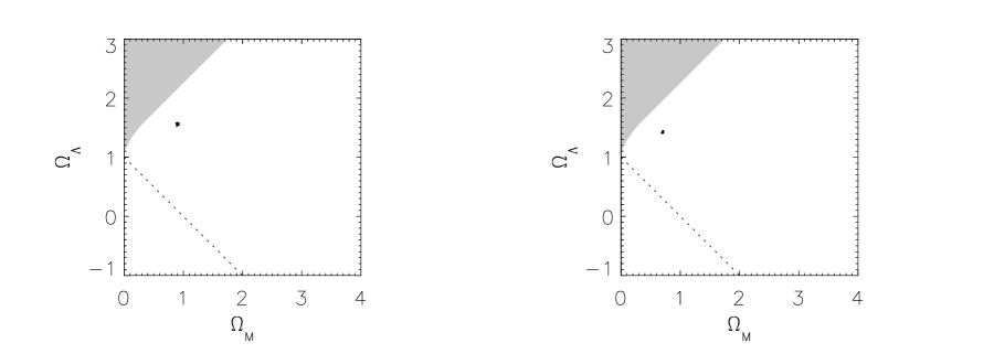
Figure 9: The scatter in the maximum likelihood estimates of $\Omega_{m}$ and $\Omega_{\Lambda}$ due to uncertainties in the MVF parameters, based on 1000 Monte Carlo realizations of the SDSS MVF. We show results for 10 and 12 CLASS E/S0 lenses (left and right panels, respectively).

4.4 Effects of evolution

We now consider how evolution in the velocity function can affect the cosmological constraints we derive. We do this by using the theoretical evolution model described in Section 2.3 together with the SDSS MVF. (In our model, the VF evolves substantially less than advocated by Chae & Mao (2003). However, our model for evolution is more in line with the findings of Ofek, Rix, & Maoz (2003).) Figure 10 shows the probability versus $\Omega_{\Lambda}$ for spatially flat cosmologies. The maximum likelihood estimate and 1$\sigma$ uncertainties are $\Omega_{\Lambda}=0.72^{+0.13}_{-0.18}$ for 10 CLASS E/S0 lenses, or $0.78^{+0.10}_{-0.16}$ for 12 E/S0 lenses (see Table 2). The image separation distribution for our evolving model is not significantly different than our non-evolving model for flat cosmologies.

Figure 10: Relative probability versus $\Omega_{\Lambda}$ for spatially flat cosmologies, using the SDSS MVF and our evolution model based on extended Press-Schechter theory.

Surprisingly, evolution appears to broaden the uncertainties on $\Omega_{\Lambda}$ without shifting the maximum likelihood value. The increase in the uncertainties is fairly straightforward to understand. The evolution model predicts that $\phi(\sigma)$ increases between $z=0$ and $z=1$ (except for rare, very massive galaxies; see Fig. 1), which would increase the optical depth. But the effect weakens as $\Omega_{\Lambda}$ increases, which partially offsets the increase in the cosmological volume and causes $\tau(\Omega_{\Lambda})$ to be less steep for the evolution model than for the no-evolution model. The Poisson errors in the lens sample (or, equivalently, in the measured value of $\tau$) therefore translate into larger uncertainties in $\Omega_{\Lambda}$. Our results confirm the suggestion by Keeton (2002a) that cosmology dependence in the evolution rate can weaken the cosmological conclusions drawn from lens statistics.

Understanding why evolution produces no shift in the maximum likelihood values is more subtle. Because the velocity function is predicted to rise from $z=0$ to $z\sim 1$ (over the relevant range of $\sigma$; see Fig. 1), we might naively expect that evolution would increase the optical depth and push us to lower values of $\Omega_{\Lambda}$. However, there are actually competing effects in the likelihood. Consider the expression for the log likelihood in eqn. 40. The maximum likelihood corresponds to the point where the derivative with respect to $\Omega_{\Lambda}$ vanishes — or where the derivatives of the first and second terms in eqn. 40 are equal. Figure 11 shows these two derivatives as a function of $\Omega_{\Lambda}$, for both non-evolving and evolving MVF models. As just mentioned, evolution flattens the dependence of the optical depth on $\Omega_{\Lambda}$, lowering the derivatives. But it affects the two terms differently, because the lens term is a sum of $\log\tau$ while the non-lens term is a sum of $\tau$ itself. The flattening effect fortuitously cancels near $\Omega_{\Lambda}\simeq 0.78$, so there is no shift in the location of the maximum likelihood. We emphasize that the almost perfect cancellation near the concordance cosmology is a coincidence; if the best-fit value of $\Omega_{\Lambda}$ were something different, then we would see evolution produce a shift in the location of maximum likelihood. But as it stands, evolution does not appear to have a strong effect on our cosmological constraints. This result is consistent with the conclusions of Rix et al. (1994) and Mao & Kochanek (1994), who used simple evolution models to argue that mergers do not significantly affect lens statistics if the progenitor and product galaxies all lie on the fundamental plane of early-type galaxies (i.e., if the kinematics features are conserved).

Figure 11: Derivatives of the two $\Omega_{\Lambda}$-dependent terms in the log likelihood, eqn. 40, for our MVF (solid lines) and evolving MVF (dashed lines) models. In each case the lower and upper curves represent the terms for non-lensed and lensed sources, respectively; the likelihood is maximized at the point where the curves cross. Jaggedness in the curves is due to numerical noise. We show results for 12 CLASS E/S0 lenses. The dotted line marks $\Omega_{\Lambda}=0.78$.

4.5 Other systematic effects

We believe that by improving the model of the deflector population and considering possible redshift evolution, we have dealt with the major systematic uncertainties in lens statistics constraints on flat cosmologies. There are, however, some additional effects that should be discussed. Further data and/or analysis will be required to account for them fully, but we can identify the direction and estimate the amplitude of the effects.

First, recall that we have assumed spherical deflectors. Huterer et al. (2004) have recently studied how lens statistics are affected by ellipticity in lens galaxies and external tidal shear from neighboring objects. They find that reasonable distributions of ellipticity and shear have surprisingly little effect on both the total optical depth and the mean image separation. Ellipticity and shear do broaden the image separation distribution slightly, but that effect is not important for cosmological constraints. In particular, Huterer et al. (2004) quantify the biases in cosmological constraints due to neglecting ellipticity and shear. They find errors of $\Delta\Omega_{M}=0.00\pm 0.01$ and $\Delta\Omega_{\Lambda}=-0.02\pm 0.01$ (where the errorbars indicate statistical uncertainties from the Monte Carlo calculation method). In other words, ellipticity and shear either do not affect the parameters at all or affect them at a level that is unimportant.

Second, recent work has suggested that neglecting lens galaxy environments can bias lens statistics. Satellite galaxies (Cohn & Kochanek 2003) and groups or clusters around lens galaxies (Keeton & Zabludoff 2004) can increase lens image separations and cross sections. Conversely, neglecting their effects (as we and nearly all other authors have done) can cause underestimates of the image separations and cross sections, and hence overestimates of $\Omega_{\Lambda}$. Poor knowledge of the distribution of lens galaxy environments prevents a detailed calculation of the effect, but Keeton & Zabludoff (2004) estimate that the shift in $\Omega_{\Lambda}$ for flat cosmologies is certainly less than 0.14 and more likely to be at the level of $\sim$0.05. Surveys to characterize lens environments are now underway, and they will make it possible to account for this effect in future lens statistics calculations.

Third, the Appendix suggests the possibility that as much as 30% of the early-type galaxy population was excluded by the Bernardi et al. (2004) sample selection, although the fraction is probably much smaller. If we assume the maximum omitted fraction, then our estimates of $\Omega_{\Lambda}$ for a flat cosmology would drop by $\sim$0.05 for the IVF model and $\sim$0.15 for the MVF model.

Finally, the most significant limitation of the CLASS sample is poor knowledge of the source redshift distribution. Chae (2003) estimates that this leads to an uncertainty (but not necessarily a bias) of $\sim$0.11 in $\Omega_{\Lambda}$.

5 Conclusions

We have derived new constraints on the cosmological parameters using the statistics of strong gravitational lenses. We have modified lens statistics calculations in two important ways. First, we point out that neglecting scatter in the Faber-Jackson relation biased the results of previous analyses of lens statistics (also see Kochanek 1994). Working with a direct measurement of the velocity dispersion distribution function removes these biases. Second, we use a theoretical model for the redshift evolution of the velocity function to study how evolution affects lens statistics. These modifications allow us to obtain more robust cosmological constraints.

We find good agreement between lens statistics and the current concordance cosmology (at 1$\sigma$) and with the recent results from Type Ia supernovae (e.g., Tonry et al. 2003). Our maximum likelihood flat cosmology for the (non-evolving) MVF model has $\Omega_{\Lambda}=0.74^{+0.09}_{-0.11}$ if 10 of the 13 CLASS lenses are produced by early-type galaxies, or $\Omega_{\Lambda}=0.78^{+0.07}_{-0.10}$ if there are 12 CLASS early-type lenses. Neglecting the scatter in the Faber-Jackson relation (using the IVF rather than the MVF) would bias the results toward higher values of $\Omega_{\Lambda}$, with a shift $\Delta\Omega_{\Lambda}\simeq 0.2$ that is twice as large as the statistical errors. If there is evolution in the velocity function that can be modeled with extended Press-Schechter theory, it has surprisingly little effect on the maximum likelihood values of $\Omega_{\Lambda}$ but it does increase the uncertainties by $\sim$50%. The Appendix suggests the Bernardi et al. (2004) sample might be missing up to 30% of early-type galaxies, but this omitted fraction is likely much smaller. If the full 30% are being omitted, then our estimates of $\Omega_{\Lambda}$ for a flat cosmology would drop by $\sim$0.05 for the IVF model and $\sim$0.15 for the MVF model.

While it is gratifying to see that lens statistics now agree with what are considered to be strong cosmological constraints from supernovae and the cosmic microwave background, one may wonder whether the lensing results are actually interesting. We believe that they are, for several reasons. Perhaps the most essential question in cosmology today is whether there is a dark energy component. To date the only single dataset able to address that question has been the supernovae. (The CMB constrains the total density $\Omega_{\Lambda}+\Omega_{m}$, while clusters constrain $\Omega_{m}$.) Perhaps the most significant result from lens statistics is strong evidence for $\Omega_{\Lambda}>0$, absent any other cosmological assumptions (see Fig. 7). With the underlying physics of Type Ia supernovae not understood, the confirmation from lensing is significant. Alternatively, if the cosmology is known and accepted from other methods, then lensing will provide perhaps the cleanest probe of dynamical evolution in the early-type galaxy population to test the paradigm of hierarchical structure formation that forms the other main pillar of our cosmological paradigm.

Appendix A Selection of the sample of early-type galaxies

The selection procedures outlined by Bernardi et al. (2003) define the sample we use in our analysis. This Appendix studies the roles played by each step in the selection process. We find that the sample could plausibly underestimate the true abundances of massive early-type galaxies of interest for lensing, but not by more than $\sim$30%. We then argue that the missed fraction is likely to be considerably smaller, based on recent measurements (Cross et al. 2004) of the early-type galaxy luminosity function at the redshifts $z\sim 0.5$–1 relevant for lensing.

We begin with an observation that SDSS data have made quite clear: to a rather surprising approximation, the galaxy distribution is bimodal (e.g., Blanton et al. (2003b)). Baldry et al. (2004) describe how the $u-r$ vs $r$ color-magnitude diagram can be used to construct an optimal division between what are essentially red and blue populations. Since it is widely accepted that giant early-type galaxies are red, they almost certainly belong to the red population. Of course, the red population may also have a substantial number of edge-on disks, so the bimodality in color almost certainly does not translate simply into a bimodality in morphology. Nevertheless, we will use this red population as a basis against which to compare the Bernardi et al. (2003) selection process.

We do this by selecting objects from the SDSS main galaxy sample, restricted to the range $13.5\leq r_{\rm Pet}\leq 17.77$ and $z\leq 0.08$, following Baldry et al. (2004). This gives 71,517 objects. The crosses in Figure 12 show our estimate of the luminosity function of this sample; it is well-described by the solid line, which shows the estimate published by Baldry et al. (2004) Selecting with the color cuts in Baldry et al. (2004) (where all magnitudes are Petrosian),

$$M_{u}-M_{r}>2.06-0.244\tanh[(M_{r}+20.07)/1.09],$$

yields a red subsamble containing 29908 objects. The crosses show our estimate of the red galaxy luminosity function, and the dashed line shows $\phi_{red}$ published by Baldry et al. (2004) Once again the agreement is reassuring, suggesting that our estimator of the luminosity function is accurate.

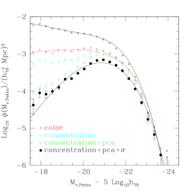
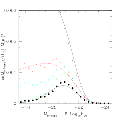
Figure 12: Luminosity functions associated with various subsamples drawn from the SDSS main galaxy sample at $z\leq 0.08$ and $13.5\leq r_{\rm Pet}\leq 17.77$ . Top set of crosses shows the luminosity function of the full sample, and the lower set is for the red subsample defined by Baldry et al. (2004); curves show their published fits to $\phi_{tot}$ and $\phi_{red}$. Triangles, squares and circles show subsamples defined by applying successive cuts in concentration, spectral type, and velocity dispersion. Bottom curve shows equation (32), shifted faintwards by 0.1 mags to account for the fact that Petrosian magnitudes used here only account for about 90% of the light in a de Vaucouleurs profile. In all cases, the luminosity function has been estimated by assuming that the sample is purely magnitude limited.

Next, we compare this sample of red galaxies with the sample selected following Bernardi et al. (2003). Because one of their goals was to study the color magnitude relation of early-type galaxies, Bernardi et al. did not select on color. Instead, they used a combination of photometric and spectroscopic cuts to define their sample. To mimic their selection, we return to the full galaxy sample, apply the same redshift and apparent magnitude cuts, and then select all objects for which the concentration index of the light profile in the $i_{\rm Pet}$ band photometry is greater than $2.75-5z/6$, where $z$ is the redshift. Use of the concentration as an indicator of galaxy type is motivated by Strateva et al. (2001), and this concentration cut is one of the cuts made by Bernardi et al. The redshift dependence is included to account for the fact that the concentration index is not seeing-corrected. The triangles show the luminosity function associated with the 23,857 galaxies which satisfy this cut: notice that it tracks $\phi_{red}$ well at the most luminous end, but that it is lower by about 0.3 dex at lower luminosities ($M_{r,{\rm Pet}}>-21$). Direct inspection of the images of a random sample of the red objects which do not satisfy the concentration cut shows that they are predominantly edge-on disks. Thus, for the purposes of selecting an early-type galaxy sample, the cut on concentration is more efficient and accurate than selecting on color.

We then applied the Bernardi et al. (2003) cut on spectral-type, obtained from a PCA analysis of the spectrum: the specific requirement is that the spectroscopic pipeline parameter eclass$<0$. This is essentially a cut on the shape of the continuum, and removes objects whose spectra indicate recent star-formation. Open squares show the luminosity function of the 17,977 objects that remain; the cut on spectral type removes many more of the lowest luminosity objects, but makes little difference at the luminous end which is most relevant for the present study.

Finally, filled circles show the luminosity function for the subset of 12,490 objects which satisfied both the concentration and spectral type cuts, and for which the spectroscopic pipeline reports a measured velocity dispersion. Velocity dispersions are only measured if the signal-to-noise ratio of pixels in particular wavelength intervals of the spectra is sufficiently high, so this final cut does not have any underlying physical motivation — it is made purely so that measured velocity dispersions are reliable. The filled circles fall about 0.2 dex below the open squares at small luminosities, but they are quite similar to the squares at the highest luminosities. This suggests that, by only including objects for which reliable velocity dispersion measurements are available, Bernardi et al. (2003) may have removed bona-fide low and moderate luminosity early-type galaxies from the sample, but it has not significantly reduced the inferred abundance of the most luminous objects. Thus, while the number density of early-type galaxies may be larger than they quote, but it is unlikely to be more than $10^{0.2}\sim 50\%$ higher at $L<L_{*}$, and it is likely to be unchanged at $L>6L_{*}$.

If the Bernardi et al. (2004) sample is missing some bona-fide early-types, then one way to quantify this is to estimate the fraction of the total luminosity density contributed by early-types. The luminosity density in the Baldry et al. (2004) red sample is 42% of the total (consistent with the red galaxy sample of Hogg et al. (2002), but this is almost certainly an overestimate of the contribution from early-type galaxies to the luminosity density. The cut on concentration rather than color leaves 39% of the total luminosity density, including the cut on spectral type reduces this to 31%, and requiring that reliable $\sigma$ measurements are available reduces this to 22%. These numbers are actually slight underestimates of the early-type contribution, because they were computed from the Petrosian luminosity, whereas the luminosity of an early-type galaxy is actually better represented by the de Vaucouleurs luminosity. As Blanton et al. (2001) demonstrate, the Petrosian luminosity underestimates the true value by about 10%. If $j_{\rm Petro}=e/(e+l)$, then correcting for this difference means that $j_{\rm deV}=1.1e/(1.1e+l)=1/(1+l/1.1e)=j_{\rm Petro}1.1/(1+0.1j_{\rm Petro})$. Hence, the early-type fractions associated with these cuts, 0.39, 0.31 and 0.22, become 0.42, 0.34, and 0.24. Since the final cut does not change the shape of the luminosity distribution drastically (the squares and circles trace curves of similar shape), it may be that the final cut leaves a sample which underestimates the true number density of ellipticals by about 30% (i.e., $1-0.24/0.34$). Therefore, it may be that the distribution of velocity dispersions $\phi(\sigma)$ in the Bernardi et al. sample accurately represents the true shape of the MVF, but underestimates the number density by a similar factor.

There is one important caveat, however: the analysis above is restricted to low redshifts. More relevant for our analysis is the distribution of velocity dispersions at typical lens redshifts, $z\sim 0.5$–1. In the IVF model, we use the $\phi(L)$ distribution measured at low redshifts and assume that the only change with redshift is pure luminosity evolution. We can test this assumption by comparing the luminosity function we use with that recently measured from 48 arcmin² of HST-ACS fields at $z\sim 0.75$ (Cross et al. 2004). Figure 13 illustrates that the number densities from the higher-redshift sample are slightly lower than those from the SDSS ‘concentration+pca+$\sigma$’ sample, and substantially lower than those from the SDSS sample in which the cut on $\sigma$ has been omitted. Therefore, using all three cuts to define the early-type sample is probably a better approximation than using only the ‘concentration+pca’ cuts.

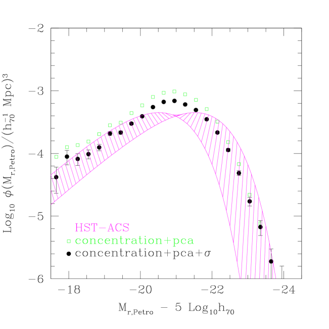
Figure 13: Early-type galaxy luminosity functions from the SDSS sample (squares and circles show subsamples defined by applying successive cuts in concentration, spectral type, and velocity dispersion, as in previous figure), and from the HST-ACS survey (hashed region shows the luminosity function of objects with $(U-V)>1.38$ and $0.5\leq z\leq 0.75$, shifted to $z=0$ assuming $M_{r}=M_{B}-1.32-1.76z_{ACS}$ with $z_{ACS}=0.65$, and assuming that $M_{*}\pm 0.5$ mags following Cross et al. 2004). The number density estimated from the high-redshift population is smaller than that estimated from lower-redshifts.

In light of these arguments, it is interesting to consider Figures 2 and 4 in the main text. If the Bernardi et al. sample does underestimate the number density of early-type galaxies and we were to increase the normalization $\phi_{*}$ to compensate, this would bring the SDSS MVF closer to the SSRS2 IVF at lower $\sigma$. However, the large-$\sigma$ tails would still differ because the SDSS MVF correctly includes the effect of scatter in the $\sigma-L$ relation. As for the SDSS IVF, since it was obtained by transforming the luminosity function, the final cut on signal-to-noise mainly affects the normalization but does not substantially change the shape of the function.

On the other hand, the IVF is also sensitive to the relation between $\sigma$ and $L$: in particular, it is sensitive to $\langle\sigma|L\rangle$. So it is interesting to compare this relation in the SDSS sample with results from the literature. Figure 14 shows this relation in the SDSS early-type sample; crosses show the median $V$ in small bins in $M_{r}$ where $M_{r}$ has been corrected for evolution to $z=0$. The solid line shows a linear fit of the form given in the panel. For comparison, the dotted line shows the fit reported by Bernardi et al. (2003), $\langle V|M_{r}\rangle=2.2-0.105(M_{r}+21.15-0.125)$, where the factor of 0.125 accounts for the new SDSS photometry. The dots show a sample of 236 early-type galaxies from the compilation of Prugniel & Simien (1996), rescaled to account for the shift in waveband (we used $M_{B}-M_{r}=1.32$ following Fukugita et al. 1995) and $H_{0}$ (they assumed $H_{0}=75$ km s^-1 Mpc^-1, whereas we use 70 km s^-1 Mpc^-1). The dashed line shows $\langle V|M_{r}\rangle$; it is similar to the fit reported by Forbes & Ponman (1999): $V=0.243-0.102[M_{r}+1.32+5{\rm Log}_{10}(75/70)]$. As a result, the $\sigma-L$ relation has larger velocity dispersions for a given luminosity than the relation we use to estimate the IVF in the main text. The reason for this difference is clear: inspection of the points suggests that the Prugniel & Simien (1996) sample has fewer luminous objects ($M_{r}<-22.5$) with low $\sigma$ than one might have expected from inspection of the distribution of objects at lower luminosities in the sample. The SDSS sample shows no such difference.

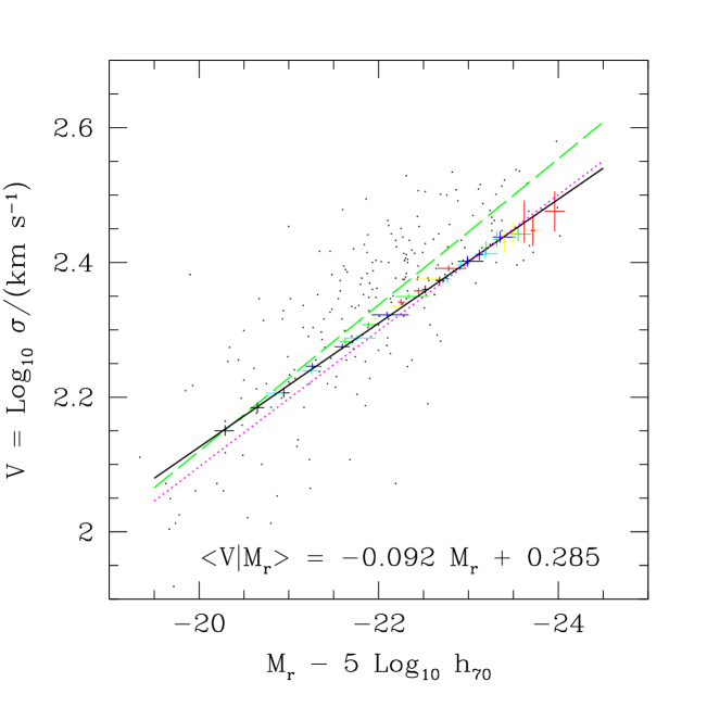
Figure 14: Correlation between velocity dispersion and luminosity. Error-bars show the SDSS early-type galaxy sample, obtained by stacking together many volume limited catalogs. Solid line shows the fit reported in the figure, and dotted line shows the fit from Bernardi et al. (2003), rescaled to account for the new photometry. Dots show a local sample of 236 early-type galaxies from Prugniel & Simien (1996), and dashed line shows a fit to their sample.

References

- Argo et al. (2003) Argo, M. K. et al. 2003, MNRAS, 338, 957
- Augusto et al. (2002) Augusto, P., et al. 2002, MNRAS, 326, 1007
- Baldry et al. (2004) Baldry, I. K., et al. 2004 ApJ, 600, 681
- Benson et al. (2003) Benson, A. J., Bower, R. G., Frenk, C. S., Lacey, C. G., Baugh, C. M., & Cole, S. 2003, ApJ, 599, 38
- Biggs et al. (2003) Biggs, A.D. et al. 2003, MNRAS, 338, 1084
- Bernardi et al. (2003) Bernardi, M., et al. [SDSS Collaboration] 2003, AJ, 125, 1817
- Bernardi et al. (2004) Bernardi, M., et al. [SDSS Collaboration] 2004, in preparation
- Blanton et al. (2001) Blanton, M. R., et al. 2001, AJ, 121, 2358
- Blanton et al. (2003) Blanton, M. R., et al. 2003, ApJ, 592, 819
- Blanton et al. (2003b) Blanton, M. R., et al. 2003b, ApJ, 594, 186
- Browne et al. (2003) Browne, I. W. A., et al. [CLASS Collaboration] 2003, MNRAS, 341, 13
- Browne et al. (1993) Browne, I. W. A., Patnaik, A. R., Walsh, D., Wilkinson, P. N. 1993, MNRAS, 263, L32
- Bryan & Norman (1997) Bryan, G. L., & Norman, M. L. 1997, ApJ, 495, 80
- Chae (2003) Chae, K.-H. 2003, MNRAS, 346, 746
- Chae & Mao (2003) Chae, K.-H., & Mao, S. 2003, ApJ, 599, L61
- Chae et al. (2002) Chae, K.-H., et al. 2002, Phys.Rev.Lett., 89, 151301
- Chae, Mao, & Augusto (2001) Chae, K.-H., Mao, S., Augusto, P. 2001, MNRAS, 326, 1015
- Cheng & Krauss (2000) Cheng, Y.-C., & Krauss, L. M. 2000, Int. J. Mod. Phys. A., A15, 697
- Chiba & Yoshii (1999) Chiba, M., & Yoshii, Y. 1999, ApJ, 510, 42
- Cohn & Kochanek (2003) Cohn, J. D., & Kochanek, C. S. 2003, preprint (astro-ph/0306171)
- Cole et al. (1994) Cole, S., Aragon-Salamanca, A., Frenk, C. S., Navarro, J. F., & Zepf, S. E. 1994, MNRAS, 271, 781
- Cooray & Huterer (1999) Cooray, A. R., & Huterer, D. 1999, ApJ, 513, L95
- Cross et al. (2004) Cross, N. J. G., et al. 2004, astro-ph/0407644
- Davis, Huterer, & Krauss (2003) Davis, A. N., Huterer, D., & Krauss, L. M. 2003, MNRAS, 344, 1029
- Fabbiano (1989) Fabbiano, G. 1989, ARA&A, 27, 87
- Falco, Kochanek, & Muñoz (1998) Falco, E. E., Kochanek, C. S., & Muñoz, J. A. 1998, ApJ, 494, 47
- Fassnacht & Cohen (1998) Fassnacht, C. D., & Cohen, J. G. 1998, AJ, 115, 377
- Fassnacht et al. (1999) Fassnacht, C. D., et al. 1999, AJ, 117, 658
- Forbes & Ponman (1999) Forbes, D. A., Ponman, T. J. 1999, MNRAS, 309, 623
- Franx (1993) Franx, M. 1993, in Galactic Bulges (IAU Symposium 153), ed. H. DeJonghe & H. J. Habing, p. 243
- Fried et al. (2001) Fried, J. W., von Kuhlmann, B., Meisenheimer, K., Rix, H.-W., Wolf, C., Hippelein, H. H., Kummel, M., Phleps, S., Roser, H. J., Thierring, I., & Maier, C. 2001, A& A, 367, 788
- Fukugita, Futamase, & Kasai (1990) Fukugita, M., Futamase, T., & Kasai, M. 1990, MNRAS, 246, 24P
- Fukugita & Turner (1991) Fukugita, M., & Turner, E. L. 1991, MNRAS, 253, 99
- Gerhard et al. (2001) Gerhard, O., Kronawitter, A., Saglia, R. P., & Bender, R. 2001, AJ, 121, 1936
- Giovanelli et al. (1997) Giovanelli, R., Haynes, M. P., Herter, T., Vogt, N. P., Wegner, G., Salzer, J. J., da Costa, L. H., & Freudling, W. 1997, AJ, 113, 22
- Helbig et al. (1999) Helbig, P., et al. 1999, AA Supp. Ser., 136, 297
- Hinshaw & Krauss (1987) Hinshaw, G., & Krauss, L. M. 1987, ApJ, 320, 468
- Hogg et al. (2002) Hogg, D. W., et al. 2002, AJ, 124, 2
- Huterer et al. (2004) Huterer, D., Keeton, C. R., & Ma, C.-P. 2004, ApJ, submitted, astro-ph/0405040
- Im et al. (2002) Im, M., et al. 2002, ApJ, 571, 136
- Jackson et al. (1998) Jackson, N., et al. 1998, MNRAS, 296, 483
- Jenkins et al. (2001) Jenkins, A., Frenk, C. S., White, S. D. M., Colberg, J. M., Cole, S., Evrard, A. E., Couchman, H. M. P., & Yoshida, N. 2001, MNRAS, 321, 372
- Kauffmann, Charlot, & White (1996) Kauffmann, G., Charlot, S., & White, S. D. M. 1996, MNRAS, 283, L117
- Kauffmann et al. (1999) Kauffmann, G., Colberg, J. M., Diaferio, A., & White, S. D. M. 1999, MNRAS, 303, 188
- Kauffmann et al. (1993) Kauffmann, G., White, S. D. M., & Guiderdoni, B. 1993, MNRAS, 264, 201
- Keeton, Kochanek, & Seljak (1997) Keeton, C. R., Kochanek, C. S., & Seljak, U. 1997, ApJ, 482, 604
- Keeton, Kochanek, & Falco (1998) Keeton, C. R., Kochanek, C. S., & Seljak, U. 1998, ApJ, 509, 561
- Keeton & Madau (2001) Keeton, C. R., & Madau, P. 2001, ApJ, 549, L25
- Keeton (2002a) Keeton, C. R. 2002a, ApJ, 575, L1
- Keeton (2002b) Keeton, C. R. 2002b, ApJ, 582, 17
- Keeton et al. (2000) Keeton, C. R., Christlein, D., & Zabludoff, A. I. 2000, ApJ, 545, 129
- Keeton & Zabludoff (2004) Keeton, C. R., & Zabludoff, A. I. 2004, ApJ, 612, 660
- King et al. (1999) King, L. J., Browne, I. W. A., Marlow, D. R., Patnaik, A. R., & Wilkinson, P. N. 1999, MNRAS, 307, 225
- Kochanek (1993) Kochanek, C. S. 1993, ApJ, 419, 12
- Kochanek (1994) Kochanek, C. S. 1994, ApJ, 436, 56
- Kochanek (1995) Kochanek, C. S. 1995, ApJ, 453, 545
- Kochanek (1996) Kochanek, C. S. 1996, ApJ, 466, 638
- Kochanek et al. (2000) Kochanek, C. S., et al. 2000, ApJ, 543, 131
- Koopmans & Treu (2003) Koopmans, L. V. E., & Treu, T. 2003, ApJ, 583, 606
- Krauss & White (1992) Krauss, L. M., White, M. 1992, ApJ, 394, 385
- Lacey & Cole (1994) Lacey, C., & Cole, S. 1994, MNRAS, 271, 676
- Li & Ostriker (2002) Li, L., & Ostriker, J. P., 2002, ApJ, 566, 652
- Lin et al. (1999) Lin, H., Yee, H. K. C., Carlberg, R. G., Morris, S. L, Sawicki, M., Patton, D. R., Wirth, G., Shepherd, C. W. 1999, ApJ, 518, 523
- Lubin et al. (2000) Lubin, L. M., Fassnacht, C. D., Readhead, A. C. S., Blandford, R. D., & Kundić, T. 2000, AJ, 119, 451
- Madgwick et al. (2002) Madgwick, D. S., et al. 2002, MNRAS, 333, 133
- Mao & Kochanek (1994) Mao, S. D., & Kochanek, C. S. 1994, MNRAS, 268, 569
- Maoz & Rix (1993) Maoz, D., & Rix, H.-W. 1993, ApJ, 416, 425
- Marlow et al. (2000) Marlow, D. R¿, Rusin, D., Jackson, N., Wilkinson, P. N., & Browne, I. W. A. 2000, AJ, 119, 2629
- Marzke et al. (1998) Marzke, R. O., da Costa, L. N., Pellegrini, P. S., Willmer, C. N. A., & Geller, M. J. 1998, ApJ, 503, 617
- McKean et al. (2004) McKean, J. P., Koopmans, L. V. E., Browne, I. W. A., Fassnacht, C. D., Blandford, R. D., Lubin, L. M., & Readhead, A. C. S. 2004, MNRAS, in press.
- Muñoz et al. (2003) Muñoz, J. A., Falco, E. E., Kochanek, C. S., Lehár, J., & Mediavilla, E. 2003, ApJ, 594, 684
- Myers et al. (1995) Myers, S. T., et al. 1995, ApJ, 447, L5
- Myers et al. (1999) Myers, S. T., et al. 1999, AJ, 117, 2565
- Myers et al. (2003) Myers, S. T., et al. [CLASS Collaboration] 2003, MNRAS, 341, 1
- Narayan & White (1988) Narayan, R., & White, S. D. M. 1988, MNRAS, 231, 97p
- Newman & Davis (2000) Newman, J. A., & Davis, M. 2000, ApJ, 534, L11
- Newman & Davis (2002) Newman, J. A., & Davis, M. 2002, ApJ, 564, 567
- Norberg et al. (2002) Norberg, P., et al. 2002, MNRAS, 336, 907
- Ofek, Rix, & Maoz (2003) Ofek, E. O., Rix, H. W., & Maoz, D. 2003, MNRAS, 343, 639
- Patnaik et al. (1992a) Patnaik, A.R., Browne, I.W.A., Wilkinson, P.N., & Wrobel, J.M. 1992a, MNRAS, 254, 655
- Patnaik et al. (1992b) Patnaik, A.R., Browne, I.W.A., Walsh, D., Chaffee, F.H., & Foltz, C.B. 1992b, MNRAS, 259P, 1
- Patnaik et al. (1993) Patnaik, A.R., Browne, I.W.A., King, L.J., Muxlow, T.W.B., Walsh, D. & Wilkinson, P.N. 1993, MNRAS, 261, 435
- Porciani & Madau (2000) Porciani, C., & Madau, P. 2000, ApJ, 532, 679
- Prugniel & Simien (1996) Prugniel, P. & Simien, F. 1996, AA, 309, 749
- Quast & Helbig (1999) Quast, R., & Helbig, P. 1999, AA, 344, 721
- Rix et al. (1997) Rix, H. W., de Zeeuw, P. T., Carollo, C. M., Cretton, N., & van der Marel, R. P. 1997, ApJ, 488, 702
- Rix et al. (1994) Rix, H.-W., Maoz, D., Turner, E. L., Fukugita, M. 1994, ApJ, 435, 49
- Rusin et al. (2001a) Rusin, D., et al. 2001a, ApJ, 557, 594
- Rusin et al. (2001b) Rusin, D., et al. 2001b, AJ, 122, 591
- Rusin, Kochanek, & Keeton (2003) Rusin, D., Kochanek, C. S., & Keeton, C. R. 2003, ApJ, 595, 29
- Rusin & Ma (2001) Rusin, D., & Ma, C.-P. 2001, ApJ, 549, L33
- Sarbu, Rusin, & Ma (2001) Sarbu, N., Rusin, D., & Ma, C.-P., 2001, ApJ, 561, L147
- Schade et al. (1999) Schade, D., et al. 1999, ApJ, 525, 31
- Schechter (1976) Schechter, P. 1976, ApJ, 203, 297
- Sheth et al. (2003) Sheth, R. K., et al., 2003, ApJ, 594, 225
- Sheth & Tormen (1999) Sheth, R. K., & Tormen, G. 1999, MNRAS, 308, 119
- Sheth, Mo & Tormen (2001) Sheth, R. K., Mo, H. J., & Tormen, G. 2001, MNRAS, 323, 1
- Somerville & Primack (1999) Somerville, R. S., & Primack, J. R. 1999, MNRAS, 310, 1087
- Spergel et al. (2003) Spergel, D. N., et al. 2003, ApJ, 148, 175
- Strateva et al. (2001) Strateva, I., et al. 2001, ApJ, 122, 1861
- Surpi & Blandford (2003) Surpi, G., & Blandford, R. D. 2003, ApJ, 584, 100
- Sykes et al. (1998) Sykes, C.M., et al. 1998, MNRAS, 301, 310
- Tonry et al. (2003) Tonry, J., et al. 2003, ApJ, 594, 1
- Totani & Yoshii (1998) Totani, T., & Yoshii, Y. 1998, ApJ, 492, 461
- Treu & Koopmans (2004) Treu, T., & Koopmans, L. V. E. 2004, astro-ph/0401373
- Treu & Koopmans (2002) Treu, T., & Koopmans, L. V. E. 2002, ApJ, 575, 87
- Turner (1990) Turner, E. L. 1990, ApJ, 365, L43
- Turner, Ostriker, & Gott (1984) Turner, E. L., Ostriker, J. P., Gott, J. R. III, 1984, ApJ, 284, 1
- Waga & Frieman (2000) Waga, I., & Frieman, J. 2000, Phys. Rev. D, 043521
- Waga & Miceli (1999) Waga, I., & Miceli, A. P. M. R. 1999, Phys. Rev. D, 59, 103507
- Wallington & Narayan (1993) Wallington, S., & Narayan, R. 1993, ApJ, 403, 517
- White & Frenk (1991) White, S. D. M., & Frenk, C. S. 1991, ApJ, 379, 52
- Winn et al. (2004) Winn, J. N., Rusin, D., & Kochanek, C. S. 2004, Nature, 427, 613
- Yasuda et al. (2001) Yasuda, N., et al. 2001, AJ, 122, 1104