The Local Ly$\alpha$ Forest IV: STIS G140M Spectra and Results on the Distribution and Baryon Content of H I Absorbers

Abstract

We present HST STIS/G140M spectra of 15 extragalactic targets, which we combine with GHRS/G160M data to examine the statistical properties of the low-$z$ Ly$\alpha$ forest. With STIS, we detect 109 Ly$\alpha$ absorbers at significance level ($SL$) $\geq 4\sigma$ over $0.002<z<0.069$, with a total redshift pathlength $\Delta z=0.770$. Our combined sample consists of 187 Ly$\alpha$ absorbers with $SL\geq 4\sigma$ over $\Delta z=1.157$. We evaluate the physical properties of these Ly$\alpha$ absorbers and compare them to their high-$z$ counterparts. Using two different models for Ly$\alpha$ forest absorbers, we determine that the warm, photoionized IGM contains $29\pm 4\%$ of the total baryon inventory at $z=0$ (assuming $J_{0}=1.3\times 10^{-23}$ ergs cm^-2 s^-1 Hz^-1 sr^-1). We derive the distribution in column density, $N_{\rm HI}$^-1.65±0.07 for $12.5\leq\log{\left[N_{\rm HI}({\rm cm}^{-2})\right]}\leq 14.5$, breaking to a flatter slope above $\log{\left[N_{\rm HI}\right]}\approx 14.5$. As with the high equivalent width ($\mathcal{W}>240~{}{\rm m}\mbox{\AA}$) absorbers, the number density of low-$\mathcal{W}$ absorbers at $z=0$ is well above the extrapolation of d$\mathcal{N}$/d$z$ from $z>2$. However, $\log\left[({\rm d}\mathcal{N}/{\rm d}z)_{z=0}\right]=1.40\pm 0.08$ for $\mathcal{W}>240~{}{\rm m}\mbox{\AA}$ is $25\%$ below the value obtained by the HST QSO Key Project, a difference that may arise from line blending. The slowing of the number density evolution of high-$\mathcal{W}$ Ly$\alpha$ clouds is not as great as previously measured, and the break to slower evolution may occur later than previously suggested ($z\sim 1.0$ rather than 1.6). We find a $7.2\sigma$ excess in the two-point correlation function (TPCF) of Ly$\alpha$ absorbers for velocity separations $\Delta v\leq 260$ km s^-1, which is exclusively due to the higher column density clouds. From our previous result that higher column density Ly$\alpha$ clouds cluster more strongly with galaxies, this TPCF suggests a physical difference between the higher and lower column density clouds in our sample. The systematic error produced by cosmic variance on these results increases the total errors on derived quantities by $\sim\sqrt{2}$.

1 Introduction

Since the discovery of the high-redshift Ly$\alpha$ forest over 30 years ago, these abundant absorption features in the spectra of QSOs have been used as evolutionary probes of the intergalactic medium (IGM), galactic halos, large-scale structure, and chemical evolution. In the past few years, these discrete Ly$\alpha$ lines have been interpreted in the context of N-body hydrodynamical models (Cen et al., 1994; Hernquist et al., 1996; Zhang et al., 1997; Davé et al., 1999) as arising from baryon density fluctuations associated with gravitational instability during structure formation. However, the detailed physical processes governing the recycling of metal-enriched gas, from galaxy disks into extended but still gravitationally-bound galaxy halos or into gravitationally-unbound winds, have not been included in these simulations to any precision. Therefore, the physical and causal relationship between the Ly$\alpha$ forest absorbers and galaxies is still uncertain and controversial (see Mulchaey & Stocke, 2002). Hubble Space Telescope (HST) UV spectroscopy with the Faint Object Spectrograph (FOS) and Goddard High Resolution Spectrograph (GHRS) in the past, with the Space Telescope Imaging Spectrograph (STIS) at present, and with the Cosmic Origins Spectrograph (COS) in the future, can make a significant contribution to this problem. This is due to the low redshift ($z<0.1$) of the absorbers discovered with HST, allowing a detailed scrutiny of the nearby galaxy distribution not possible at high-$z$.

At high redshift, the Ly$\alpha$ absorption lines evolve rapidly with redshift, $d{\cal N}/dz\propto(1+z)^{\gamma}$, where $\gamma\approx 2.2$ for $1.5\leq z\leq 4$ (Kim et al., 2001). A major surprise came when HST discovered Ly$\alpha$ absorption lines toward the quasar 3C 273 at $z_{\rm em}=0.158$, using both FOS (Bahcall et al., 1991) and GHRS (Morris et al., 1991, 1993). The number of these absorbers was far in excess of their expected number based upon an extrapolation from high-$z$ (Weymann et al., 1998). Current evidence suggests that the evolution of the Ly$\alpha$ forest slowed dramatically at $z<1.6$, probably as a result of the collapse and assembly of baryonic structures in the IGM together with the decline in the intensity of the ionizing radiation field (Theuns, Leonard, & Efstathiou, 1998; Davé et al., 1999; Haardt & Madau, 1996; Shull et al., 1999b). Detailed measurements of the Ly$\alpha$ forest evolution in the interval $z<1.5$, for equivalent widths $\mathcal{W}>240~{}{\rm m}\mbox{\AA}$, are described in the FOS Key Project papers: the three catalog papers (Bahcall et al., 1993, 1996; Jannuzi et al., 1998) and the evolutionary analysis (Weymann et al., 1998).

In previous papers in our series (Penton, Stocke, & Shull, 2000a; Penton, Shull, & Stocke, 2000b; Penton, Stocke, & Shull, 2002, Papers I, II, III, respectively), we used the HST/GHRS and the G160M first-order grating with $\sim$19 km s^-1 resolution to study the very low-redshift ($z<0.07$) Ly$\alpha$ forest at lower column densities than was possible with the Key Project data (our limiting $\mathcal{W}$ is $\sim$15 mÅ  or $\log{\left[N_{\rm HI}({\rm cm}^{-2})\right]}\geq 12.5$; hereafter, $N_{\rm HI}$ is implied to be in units of  cm^-2). Paper II showed that the number density evolution of low-$N_{\rm HI}$ Ly$\alpha$ forest absorbers also exhibits a rapid decline from higher redshift, but perhaps with only a minimal slowing in that evolution at $z\sim 1$. These low $N_{\rm HI}$  absorbers show a small excess power in the cloud-cloud two-point correlation function (TPCF) amplitude and only at $c\Delta z\leq 150$ km s^-1 (Paper II). Unlike results based on ground-based galaxy surveys near the high-$N_{\rm HI}$ FOS absorbers (Lanzetta et al., 1995; Chen et al., 1998), the low column density absorbers do not correlate closely with galaxies (Paper III). In our GHRS sample, we found that $22\pm 8$% of the absorbers “reside” in galaxy voids. Even the remaining 78% of the absorbers are not close to galaxies, but may align with large-scale structures of galaxies (Paper III) as predicted by recent simulations (Cen et al., 1994; Davé et al., 1999). Thus, just as at high-$z$, there appears to be a physical distinction between the higher column density absorbers ($\log{\left[N_{\rm HI}\right]}\geq 14$) discovered in the Key Project work and the lower column density absorbers investigated in Papers I–III. Earlier results from our study have appeared in various research papers and reviews (Stocke et al., 1995; Shull, 1997; Shull, Penton, & Stocke, 1999a; Stocke, 2002; Stocke, Penton, & Shull, 2003; Shull, 2002, 2003).

In this paper we more than double our Ly$\alpha$ sample using 15 STIS targets. Combining these STIS/G140M results with the GHRS sample analyzed in Paper II, we confirm and extend our previous results and improve the statistics of our conclusions concerning the local Ly$\alpha$ forest. However, despite the much improved statistics, cosmic variance in absorber numbers and properties may still be an important, although diminished, factor in the error analysis. We also obtain several new results: (1) an inconclusive search for very broad, shallow absorbers in these spectra (see § 2.1); (2) a more accurate determination (§ 5.2) of the evolution in number density of high and low column density absorbers, which differs from the Key Project in suggesting that the fast evolution of higher column density absorbers may persist to $z\sim 1$; (3) a more accurate accounting of the baryon density in the local Ly$\alpha$ absorbers using two different formulations (§ 6); and (4) a separate cloud-cloud TPCF for higher and lower column density absorbers in our sample, which shows a difference in clustering (§ 7).

This paper is organized as follows. In § 2, we present the target sample and describe the basic data reduction and analysis process. We also discuss the limitations of these data for obtaining $b$-values. In § 3 and § 4, we discuss the basic properties of our measured rest-frame equivalent width ($\mathcal{W}$) and H I column density ($N_{\rm HI}$) distributions for our Ly$\alpha$ absorbers and compare them to higher-$z$ distributions. In § 5, we discuss the $z$ distribution of the low-$z$ Ly$\alpha$ forest within the small redshift range ($0.002<z<0.069$) of our spectra, as well as the cumulative Lyman continuum opacity of these absorbers and the $z$ evolution in the number density of lines, d$\mathcal{N}$/d$z$. In § 6 we present a new accounting of the local IGM baryon density which finds $29\pm 4\%$ of the baryons in the photoionized Ly$\alpha$ absorbers. In § 7, we analyze the cloud-cloud TPCF for low-$z$ Ly$\alpha$ clouds. Section 8 summarizes the important conclusions of this investigation. The spectra and the detailed line list are presented in an Appendix. As in our previous work, we assume a Hubble constant of $H_{0}$$=70h_{70}$ km s^-1 Mpc^-1.

2 The HST/STIS+G140M Sample and Spectral Processing

In Table 1 we present the basic physical data for the 15 STIS sightlines observed and analyzed in this program. This table summarizes the J2000 positions in celestial and Galactic coordinate frames (columns 2-7) and emission-line redshifts ($z$; column 8) of our HST targets. All redshifts are the optical, narrow emission line redshifts as reported from the NASA/IPAC Extragalactic Database (NED). Also included in Table 1, but discussed in detail later, are by column: (9) the adjustment required to convert the observed wavelength scale to the Local Standard of Rest (LSR), where $\Delta V_{\rm lsr}~{}=V_{\rm lsr}~{}-V_{\rm obs}$, is determined from the location of the available Galactic absorption lines (see Paper I); (10) the order ($O$) of the polynomial used to normalize the continuum of each target, and (11) the mean signal-to-noise ratio (SNR) of each spectrum per 3.22 pixel (41.2 km s^-1 full width at half maximum, FWHM) resolution element (RE). The Galactic H I LSR velocity measurements are taken from the Leiden/Dwingeloo surveys (LDS, Hartmann & Burton, 1997) for all targets except for PKS 2005-489, which we obtained from the Parkes HIPASS (Koribalski, 2002) survey. The LDS velocities have an estimated uncertainty of $\pm 2$ km s^-1, while the HIPASS data have $\pm 5$ km s^-1.

Table 1: Our 15 HST/STIS/G140M Targets

Target	RA	DEC	RA	DEC	l	b	$z$	$\Delta V_{\rm lsr}~{}$	$O$	SNR
	(hh:mm:ss)	(dd:mm:ss)	(∘)	(∘)	(∘)	(∘)		(km s-1)
(1)	(2)	(3)	(4)	(5)	(6)	(7)	(8)	(9)	(10)	(11)
HE1029-140	10 31 54.3	-14 16 52.4	157.976	-14.281	-100.67	36.51	0.0860	23.0	19	19.6
IIZW136	21 32 27.8	+10 08 19.5	323.116	10.139	63.67	-29.07	0.0630	26.9	22	21.0
MR2251-178	22 54 05.9	-17 34 55.3	343.524	-17.582	46.20	-61.33	0.0644	8.9	13	27.5
MRK478	14 42 07.5	+35 26 22.5	220.531	35.440	59.24	65.03	0.0791	17.6	21	24.8
MRK926	23 04 43.5	-08 41 08.4	346.181	-8.686	64.09	-58.76	0.0473	22.0	29	8.0
MRK1383	14 29 06.4	+01 17 05.1	217.277	1.285	-10.78	55.13	0.0865	32.4	11	24.2
NGC985	02 34 37.7	-08 47 15.7	38.657	-8.788	-179.16	-59.49	0.0431	4.0	23	21.1
PG0804+761	08 10 58.6	+76 02 42.6	122.744	76.045	138.28	31.03	0.1000	15.4	19	26.6
PG1116+215	11 19 08.7	+21 19 17.8	169.786	21.322	-136.64	68.21	0.1763	22.8	3	19.1
PG1211+143	12 14 17.7	+14 03 12.0	183.574	14.053	-92.45	74.31	0.0809	12.9	17	20.2
PG1351+640	13 53 15.8	+63 45 45.1	208.316	63.763	111.89	52.02	0.0882	10.3	24	15.3
PKS2005-489	20 09 25.5	-48 49 54.3	302.356	-48.832	-9.63	-32.60	0.0710	-3.2	8	37.5
TON-S180	00 57 20.0	-22 22 56.3	14.333	-22.382	139.00	-85.07	0.0620	-5.8	22	20.8
TON-1542	12 32 03.6	+20 09 29.3	188.015	20.158	-90.56	81.74	0.0630	17.5	29	16.8
VIIZW118	07 07 13.1	+64 35 58.3	106.805	64.600	151.36	25.99	0.0797	20.5	8	19.9

Our STIS spectra were recalibrated on September 21, 2002 using version V3.0 of STSDAS and V2.13b of CALSTIS via on-the-fly recalibration (OTFR) from the HST archive. Our observations were performed with the $52\arcsec\times 0.2\arcsec$ aperture, in either the 1195–1248 Å or 1245–1299 Å settings. For all objects except VII ZW 118 (catalog ) both settings were used for each object. In general, the post-processing of our STIS spectra was identical to the procedures used for our GHRS sample (Paper I). The differences in the procedures for handling STIS data compared to the GHRS are:

• The 1195 Å cutoff in the lower STIS setting allows us to identify Galactic N I $\lambda\lambda$1199.5, 1200.2, 1200.7, and Si III $\lambda$1206.5 absorption lines. The N I lines contribute to the determination and adjustment of our spectra to the local standard of rest (LSR).

• Owing to concerns regarding the RE (see below), all spectral fits were performed on the raw data. In our GHRS sample, spectral fits were performed on data smoothed to the approximate spectral resolution.

• Continuum normalization was performed by constructing a polynomial of the order given in Table 1, combined with Gaussian components for emission intrinsic to the target QSO (Ly$\alpha$, N I $\lambda$1134.9, and C III $\lambda$1175.7, when present) and a Galactic Ly$\alpha$ absorption component. The specific emission components included for each target are given in the Appendix.

• Based upon the 3$\sigma$ difference between the $\mathcal{W}$s of features measured prior to and after our continuum normalization, we added a 4.2% uncertainty in $\mathcal{W}$ in quadrature. In our GHRS sample we added a 3.4% continuum-level uncertainty.

Owing to the fact that the STIS 0.2″ slit corresponds to a velocity shift of $\pm 40$ km s^-1 (from a centered target), we have chosen not to use the heliocentric velocities provided by the standard reduction software. Instead, we use the strong, low ionization Galactic absorption lines of N I, S II, and Si II present in our spectra to provide a velocity zero point. We assume that these lines occur at the same LSR velocity as the dominant H I emission in that direction. As with our GHRS reduction, we expect that the wavelengths and recession velocities quoted in Table 2 and in the Appendix have accuracies of at least $\pm 5$ km s^-1 . The limitation is the accuracy with which $V_{\rm lsr}$(H I) can be determined from the 21 cm H I emission line profile and the assumed correspondence between the H I and the gas that gives rise to the Galactic metal absorption lines listed above.

For our bandpass, grating, and aperture, the STIS data handbook reports that the spectral RE, defined as the FWHM of the line spread function (LSF), is $\sim$1.7 (0.05 Å) pixels at 1200 Å ($\sim 21$ km s^-1). As shown in Figure 1, the actual LSF has considerable wings (solid line), and is best modeled as a combination of two Gaussian components of approximately equal strengths. The two components have FWHMs of 1.12 and 4.94 pixels, corresponding to Gaussian widths, $\sigma_{2a}$ and $\sigma_{2b}$ in Figure 1, of 0.47 and 2.10 pixels respectively. The best-fit single Gaussian component, also shown in Figure 1, has a FWHM of 3.22 pixels ($\sim$$41.2$ km s^-1), corresponding to a Gaussian width, $\sigma_{1}$, of 1.37 pixels (17.5 km s^-1). We believe this to be the best value for approximating the STIS spectral RE using a single-Gaussian fit, not the 1.7-pixel value obtained from the STIS instrument handbook. This RE is used to determine the significance levels ($SL$s) and $b$-values of our absorption features (see Paper I), but it does not affect the measured $\mathcal{W}$s. Choosing to use this single Gaussian approximation slightly underestimates the $SL$s of narrow absorption features in our sample, but it does not affect the $\mathcal{W}$s.

Figure 1: The solid line displays the LSF at 1200 Å for STIS/G140M and the $52\arcsec\times 0.2\arcsec$ aperture. The LSF is best modeled as the combination of two Gaussian components of approximately equal strengths with FWHMs of 1.12 and 4.94 pixels ($\sigma_{2a}$=0.47 pixels, $\sigma_{2b}$=2.10 pixels), shown as the dot-dashed Gaussians. The best-fit single Gaussian component, shown as the dashed line, has a FWHM of 3.22 pixels ($\sigma_{1}$=1.37 pixels). We use this latter value for the RE when calculating the significances and $b$-values of our absorption features.

Doppler widths and $b$-values are estimated from the velocity widths (W_G=$b_{\rm obs}$/$\sqrt{2}$) of our fitted Gaussian components to the unsmoothed spectra. As such, they are not true measurements of the actual $b$-values, as when fitting Voigt profiles or determining a curve of growth, but rather velocity dispersions assuming that the Ly$\alpha$ absorption lines may contain multiple velocity components (Shull et al., 2000) and are not heavily saturated. The latter is a particularly good assumption for the large number of low-$\mathcal{W}$ lines ($\mathcal{W}<75$ mÅ), but it becomes increasingly suspect for the higher $\mathcal{W}$ lines. Unlike our GHRS analysis, owing to the uncertainty in accurately characterizing the STIS LSF, we elected not to smooth our data with the LSF prior to fitting the components. Thus, our observed $b$-value ($b_{\rm obs}$) is simply the convolution of the instrumental profile ($b_{LSF}$) and the actual $b$-value ($b$) of the absorber. The $b$-values add in quadrature, $b^{2}=b_{\rm obs}^{2}-b_{LSF}^{2}=2({\bf W}_{G}^{2}-\sigma_{1}^{2})$. Therefore, we are hampered in detecting Ly$\alpha$ absorbers with observed $b$-values near or below $b_{\rm obs}=\sqrt{2}~{}\sigma_{1}\approx 25$ km s^-1.

Motion of the target in the STIS aperture during our lengthy exposures further broadens the LSF. In an attempt to correct for this, the jitter files from the HST observations were used to degrade the LSF in a manner unique for each observation. For our data, the removal of the jitter appears to be imperfect due to the potentially large amplitude (the 0.2″ slit width corresponds to $\sim$80 km s^-1 in our bandpass) and the incomplete details of the temporal extent of large jitter excursions. Nevertheless, for each observation, the degradation of the LSF was simulated, measured, and removed in quadrature from our observed $b$-values. Tables 2 and 6 present these corrected $b$-values. A comparison between the STIS/G140M $b$-values and the GHRS/G160M $b$-values in Paper I reveals that the STIS values are significantly larger (factor $\sim$1.5 in both the median and the mean) than the GHRS values. Since some of these same targets were observed with the STIS E140M, direct comparisons of $b$-values for $\sim$$40$ Ly$\alpha$ absorbers are currently available to us. While the dispersion is substantial, the $b$-values reported here are $\sim$2 times larger than those measured from the higher resolution HST/STIS echelle spectra. We attribute this difference to spacecraft drift and residual jitter that we were unable to remove. Additionally, at the time of our observations, the HST drift rate for a typical exposure was $\geq 0.02\arcsec$, or $10$ km s^-1 per hour for the G140M. Therefore, we consider these $b$-values suspect and do not use them in any analysis.

Making an accurate measurement of $b$-values is important in determining the actual H I column densities ($N_{\rm HI}$) of the saturated Ly$\alpha$ absorbers, since each $b$-value produces a different curve of growth for the upper range of column densities in our sample. It has been shown that the only reliable method of deriving $b$-values for partially saturated Ly$\alpha$ forest lines is by a curve-of-growth using higher Lyman series lines (Hurwitz et al., 1998; Shull et al., 2000). Significantly lower $b$-values (factor of 2 in the median) are found from the curve-of-growth technique (Shull et al., 2000). For example, the 1586 km s^-1 absorber in the 3C 273 (catalog ) sightline has $b=72$ km s^-1 from the Ly$\alpha$ profile (Weymann et al., 1995), while the curve of growth value is 16 km s^-1 (Sembach et al., 2001). The column density estimates based upon these $b$-values differ by a factor of 40. This disagreement in estimating $b$-values can be understood if the Ly$\alpha$ absorption profiles include non-thermal broadening from cosmological expansion and infall, arising from velocity shear and a few unresolved velocity components. Hu et al. (1995) reach the same conclusion, based upon $z\sim 3$ Keck HIRES QSO spectra. Therefore, given the difficulties in measuring the LSFs for individual or co-added spectra and in interpreting the $b$-values derived from them, we elect to assume a constant $b$-value of 25 km s^-1 as in Paper II. This $b$-value is similar to the median value found in a higher resolution study of $z=0$ Ly$\alpha$ absorbers by Davé & Tripp (2001). We avoid all analyses using the individual $b$-values in Tables 2 and 6, and we strongly suggest that others do the same. In Table 2 we list column densities for the Ly$\alpha$ absorbers with $b$-values of 20, 25, and 30 km s^-1 to illustrate the uncertainties in the inferred column densities.

In Appendix A, we present the STIS spectra, including sensitivity and available pathlength estimates and descriptions of relevant Galactic and extragalactic data for each spectrum, as well as a list of all absorption lines. We quote scientific results for the $SL\geq 4\sigma$ sample. We have verified that the noise characteristics of our spectra are Gaussian distributed around the continuum fits shown on the spectra in the Appendix. Given the number of independent REs in our spectra, we expect that 10% or $\sim$5 of the $3\sigma\leq SL<4\sigma$ absorption lines are likely to be spurious, while $\lesssim 0.1\%$ spurious absorptions would be expected in our $SL\geq 4\sigma$ sample. To ensure that our study examines only the IGM, as explained in Paper I, we exclude all Galactic metal-line absorbers and absorbers “intrinsic” to the AGN, with $(cz_{AGN}-cz_{abs})<1200$ km s^-1, to create the STIS Ly$\alpha$ $SL\geq 4\sigma$ sample, presented in Table 2. Owing to the substantial breadth of the Ly$\alpha$ absorptions intrinsic to the AGN, metal lines in these systems can be at redshifts significantly displaced ($\pm 100$ km s^-1) from the best-fit redshifts for Ly$\alpha$. This is particularly true when the Ly$\alpha$ absorptions are significantly blended, making precise wavelength determination of components problematical. Using a relaxed criterion for association of Ly$\alpha$ and metal line absorbers ($\pm 100$ km s^-1), we have searched for metal lines associated with intrinsic absorbers. Usually, these lines fall outside our observed waveband or the intrinsic absorber is weak or absent. However, we now identify three weak absorbers at 1241.62, 1242.25 and 1244.38 Å in the MRK 279 (catalog ) sightline as intrinsic Si III $\lambda$1206.5. Higher resolution STIS echelle observations of this target confirm these revised identifications (Arav, private communication). Similarly, two weak, intrinsic Si III absorptions are present in the MR 2251-178 (catalog ) sightline. While these identifications are slightly more uncertain than the others in Table 6 (due to the relaxed wavelength criterion), there are so few of them that they do not alter the statistical results presented here.

By column, Table 2 lists: (1) target name; (2) LSR-adjusted absorber wavelength and error in Å; these errors include the Gaussian centroid measurement error added in quadrature with the estimated $\pm 5$ km s^-1 error in setting the wavelength scale zero point (see above); (3) absorber recession velocity, $cz$ in km s^-1; (4) observed $b$-value ($b_{\rm obs}$) in km s^-1; (5) resolution-corrected $b$-value in km s^-1; (6) rest-frame equivalent width in mÅ with the total uncertainty as previously described; (7-9) estimated column densities in cm^-2 assuming $b$-values of 20, 25, 30 km s^-1; and (10) significance levels ($SL$) of each absorber in our STIS sample. A similar table for our GHRS sample of Ly$\alpha$ absorbers can be found in Paper II, Table 1. As described in Paper I, the uncertainties, $\Delta$$\mathcal{W}$, for the $\mathcal{W}$ values are from the Gaussian fit to each feature and are not the significance level, $SL$, of the absorption feature; typically $\mathcal{W}/\Delta\mathcal{W}<SL$.

Table 2: H I Column Densities ($N_{\rm HI}$) of $SL\geq 4\sigma$ Ly$\alpha$ features

Target	Wavelength	Velocity	$b_{\rm obs}$	$b$	$\mathcal{W}$	$N_{\rm HI}$			SL
Name	(Å)	(km s-1)	(km s-1)	(km s-1)	(mÅ)	$b$=20	$b$=25	$b$=30
HE1029-140	1223.66 $\pm$ 0.04	1971 $\pm$ 11	59 $\pm$ 9	53 $\pm$ 10	110 $\pm$ 39	13.46	13.42	13.40	10.1
HE1029-140	1224.60 $\pm$ 0.04	2202 $\pm$ 10	43 $\pm$ 14	35 $\pm$ 17	45 $\pm$ 31	12.97	12.96	12.95	4.5
HE1029-140	1225.50 $\pm$ 0.04	2423 $\pm$ 9	49 $\pm$ 4	42 $\pm$ 5	183 $\pm$ 32	13.84	13.75	13.70	17.9
HE1029-140	1234.01 $\pm$ 0.06	4523 $\pm$ 15	58 $\pm$ 17	52 $\pm$ 19	59 $\pm$ 37	13.11	13.09	13.08	6.4
HE1029-140	1277.99 $\pm$ 0.04	15369 $\pm$ 10	51 $\pm$ 23	44 $\pm$ 26	30 $\pm$ 32	12.78	12.78	12.77	4.2
HE1029-140	1278.38 $\pm$ 0.04	15464 $\pm$ 9	48 $\pm$ 3	42 $\pm$ 3	278 $\pm$ 26	14.50	14.17	14.03	38.0
HE1029-140	1292.47 $\pm$ 0.05	18941 $\pm$ 12	43 $\pm$ 11	36 $\pm$ 13	38 $\pm$ 20	12.88	12.88	12.87	5.5
HE1029-140	1293.35 $\pm$ 0.04	19157 $\pm$ 10	38 $\pm$ 5	30 $\pm$ 7	62 $\pm$ 18	13.13	13.11	13.10	9.4
IIZW136	1249.41 $\pm$ 0.03	8320 $\pm$ 7	41 $\pm$ 3	33 $\pm$ 4	192 $\pm$ 22	13.90	13.79	13.73	27.2
IIZW136	1264.67 $\pm$ 0.04	12084 $\pm$ 9	38 $\pm$ 5	29 $\pm$ 7	71 $\pm$ 21	13.21	13.19	13.17	9.6
IIZW136	1265.52 $\pm$ 0.04	12294 $\pm$ 9	50 $\pm$ 12	44 $\pm$ 14	52 $\pm$ 27	13.05	13.03	13.02	7.0
IIZW136	1272.55 $\pm$ 0.03	14026 $\pm$ 8	37 $\pm$ 4	27 $\pm$ 6	72 $\pm$ 19	13.21	13.19	13.18	10.4
IIZW136	1285.80 $\pm$ 0.03	17293 $\pm$ 7	83 $\pm$ 3	79 $\pm$ 3	486 $\pm$ 23	16.74	15.77	15.11	105.3
MR2251-178	1224.74 $\pm$ 0.04	2237 $\pm$ 11	21 $\pm$ 7	$<20$	39 $\pm$ 34	12.90	12.89	12.89	4.1
MR2251-178	1224.96 $\pm$ 0.06	2291 $\pm$ 14	36 $\pm$ 14	26 $\pm$ 20	52 $\pm$ 46	13.04	13.03	13.02	5.6
MR2251-178	1227.98 $\pm$ 0.05	3035 $\pm$ 13	52 $\pm$ 13	46 $\pm$ 15	60 $\pm$ 32	13.11	13.10	13.08	6.5
MR2251-178	1228.67 $\pm$ 0.04	3205 $\pm$ 10	73 $\pm$ 4	69 $\pm$ 4	349 $\pm$ 37	15.21	14.61	14.32	38.7
MR2251-178	1233.38 $\pm$ 0.04	4368 $\pm$ 11	55 $\pm$ 17	49 $\pm$ 19	40 $\pm$ 28	12.92	12.91	12.90	4.8
MR2251-178	1252.25 $\pm$ 0.04	9021 $\pm$ 11	40 $\pm$ 10	32 $\pm$ 13	51 $\pm$ 28	13.04	13.02	13.01	6.6
MR2251-178	1255.14 $\pm$ 0.04	9735 $\pm$ 10	50 $\pm$ 3	43 $\pm$ 3	181 $\pm$ 23	13.83	13.74	13.69	24.0
MR2251-178	1257.74 $\pm$ 0.04	10375 $\pm$ 11	69 $\pm$ 24	65 $\pm$ 25	38 $\pm$ 30	12.89	12.88	12.87	5.5
MR2251-178	1272.86 $\pm$ 0.04	14103 $\pm$ 11	29 $\pm$ 7	$<20$	20 $\pm$ 10	12.58	12.58	12.58	4.4
MR2251-178	1278.80 $\pm$ 0.04	15569 $\pm$ 10	21 $\pm$ 5	$<20$	17 $\pm$ 8	12.51	12.50	12.50	4.2
MR2251-178	1280.48 $\pm$ 0.04	15982 $\pm$ 10	36 $\pm$ 5	26 $\pm$ 7	30 $\pm$ 9	12.77	12.77	12.76	8.2
MRK478	1222.09 $\pm$ 0.04	1582 $\pm$ 10	52 $\pm$ 4	45 $\pm$ 4	194 $\pm$ 31	13.90	13.79	13.74	22.5
MRK478	1251.31 $\pm$ 0.04	8788 $\pm$ 10	63 $\pm$ 3	58 $\pm$ 3	290 $\pm$ 30	14.61	14.24	14.08	39.3
MRK478	1295.12 $\pm$ 0.04	19593 $\pm$ 10	49 $\pm$ 5	43 $\pm$ 6	84 $\pm$ 18	13.30	13.27	13.26	16.2
MRK926	1245.05 $\pm$ 0.05	7245 $\pm$ 12	70 $\pm$ 14	66 $\pm$ 14	179 $\pm$ 75	13.83	13.73	13.69	9.7
MRK926	1246.07 $\pm$ 0.06	7496 $\pm$ 15	51 $\pm$ 17	45 $\pm$ 20	72 $\pm$ 53	13.21	13.19	13.18	4.4
MRK926	1255.11 $\pm$ 0.05	9726 $\pm$ 12	42 $\pm$ 11	33 $\pm$ 14	77 $\pm$ 44	13.25	13.23	13.21	4.8
MRK926	1256.28 $\pm$ 0.10	10015 $\pm$ 23	77 $\pm$ 32	73 $\pm$ 34	66 $\pm$ 61	13.17	13.15	13.14	4.4
MRK926	1263.19 $\pm$ 0.04	11720 $\pm$ 9	33 $\pm$ 3	22 $\pm$ 5	117 $\pm$ 25	13.50	13.46	13.43	11.4
MRK1383	1244.44 $\pm$ 0.03	7094 $\pm$ 8	36 $\pm$ 6	26 $\pm$ 8	54 $\pm$ 19	13.06	13.05	13.04	7.3
MRK1383	1245.51 $\pm$ 0.04	7359 $\pm$ 9	39 $\pm$ 7	31 $\pm$ 10	35 $\pm$ 15	12.85	12.84	12.84	6.8
MRK1383	1250.10 $\pm$ 0.03	8490 $\pm$ 8	69 $\pm$ 4	65 $\pm$ 5	218 $\pm$ 30	14.05	13.90	13.82	30.7
MRK1383	1251.97 $\pm$ 0.04	8951 $\pm$ 10	55 $\pm$ 9	49 $\pm$ 10	66 $\pm$ 22	13.16	13.14	13.13	9.5
MRK1383	1257.20 $\pm$ 0.05	10242 $\pm$ 12	59 $\pm$ 14	53 $\pm$ 15	54 $\pm$ 27	13.06	13.05	13.04	7.7
MRK1383	1261.28 $\pm$ 0.04	11247 $\pm$ 9	49 $\pm$ 9	42 $\pm$ 10	61 $\pm$ 24	13.13	13.11	13.10	8.5
MRK1383	1278.79 $\pm$ 0.03	15566 $\pm$ 8	52 $\pm$ 3	46 $\pm$ 3	282 $\pm$ 20	14.53	14.19	14.05	45.9
MRK1383	1280.08 $\pm$ 0.07	15883 $\pm$ 18	36 $\pm$ 26	27 $\pm$ 34	26 $\pm$ 31	12.71	12.70	12.70	4.2
MRK1383	1283.15 $\pm$ 0.06	16640 $\pm$ 15	50 $\pm$ 18	44 $\pm$ 20	25 $\pm$ 20	12.70	12.69	12.69	4.1
NGC985	1224.41 $\pm$ 0.08	2156 $\pm$ 19	66 $\pm$ 25	61 $\pm$ 27	51 $\pm$ 42	13.03	13.02	13.01	4.5
PG0804+761	1220.32 $\pm$ 0.05	1147 $\pm$ 11	46 $\pm$ 4	38 $\pm$ 4	165 $\pm$ 29	13.75	13.67	13.63	18.9
PG0804+761	1221.87 $\pm$ 0.05	1530 $\pm$ 12	51 $\pm$ 9	45 $\pm$ 10	78 $\pm$ 28	13.25	13.23	13.22	10.5
PG0804+761	1222.24 $\pm$ 0.05	1621 $\pm$ 11	40 $\pm$ 11	32 $\pm$ 15	41 $\pm$ 27	12.92	12.91	12.91	5.6
PG0804+761	1238.18 $\pm$ 0.04	5552 $\pm$ 11	56 $\pm$ 3	50 $\pm$ 4	324 $\pm$ 44	14.95	14.44	14.21	58.5
PG0804+761	1238.61 $\pm$ 0.05	5658 $\pm$ 11	48 $\pm$ 43	41 $\pm$ 51	28 $\pm$ 33	12.74	12.73	12.73	5.0
PG0804+761	1247.62 $\pm$ 0.04	7880 $\pm$ 11	22 $\pm$ 5	$<20$	18 $\pm$ 9	12.53	12.53	12.53	4.2
PG0804+761	1287.02 $\pm$ 0.05	17597 $\pm$ 12	53 $\pm$ 7	47 $\pm$ 8	72 $\pm$ 21	13.21	13.19	13.18	12.0
PG0804+761	1287.68 $\pm$ 0.05	17758 $\pm$ 13	43 $\pm$ 10	36 $\pm$ 11	38 $\pm$ 18	12.88	12.87	12.87	6.3
PG0804+761	1289.98 $\pm$ 0.05	18326 $\pm$ 11	26 $\pm$ 5	$<20$	37 $\pm$ 14	12.87	12.86	12.85	6.1
PG0804+761	1292.38 $\pm$ 0.05	18918 $\pm$ 12	40 $\pm$ 9	32 $\pm$ 11	34 $\pm$ 17	12.83	12.82	12.82	5.8
PG1116+215	1221.75 $\pm$ 0.04	1499 $\pm$ 9	58 $\pm$ 11	52 $\pm$ 12	82 $\pm$ 33	13.28	13.26	13.24	8.6
PG1116+215	1235.59 $\pm$ 0.03	4913 $\pm$ 8	39 $\pm$ 7	30 $\pm$ 9	90 $\pm$ 32	13.33	13.31	13.29	9.4
PG1116+215	1250.21 $\pm$ 0.03	8518 $\pm$ 8	51 $\pm$ 3	45 $\pm$ 4	227 $\pm$ 32	14.11	13.94	13.85	27.2
PG1116+215	1254.99 $\pm$ 0.03	9696 $\pm$ 8	35 $\pm$ 8	25 $\pm$ 11	68 $\pm$ 34	13.18	13.16	13.15	8.8
PG1116+215	1265.78 $\pm$ 0.12	12357 $\pm$ 30	92 $\pm$ 37	89 $\pm$ 39	88 $\pm$ 82	13.32	13.29	13.28	10.6
PG1116+215	1266.47 $\pm$ 0.21	12529 $\pm$ 51	83 $\pm$ 53	80 $\pm$ 55	44 $\pm$ 53	12.96	12.95	12.94	5.4
PG1116+215	1269.61 $\pm$ 0.06	13301 $\pm$ 16	87 $\pm$ 21	83 $\pm$ 22	65 $\pm$ 34	13.16	13.14	13.13	8.3
PG1116+215	1287.44 $\pm$ 0.03	17698 $\pm$ 7	56 $\pm$ 5	51 $\pm$ 6	167 $\pm$ 31	13.76	13.68	13.64	20.0
PG1116+215	1289.58 $\pm$ 0.04	18227 $\pm$ 9	45 $\pm$ 8	38 $\pm$ 9	77 $\pm$ 28	13.25	13.22	13.21	8.9
PG1116+215	1291.75 $\pm$ 0.07	18763 $\pm$ 16	62 $\pm$ 21	57 $\pm$ 23	42 $\pm$ 31	12.94	12.93	12.92	4.8
PG1211+143	1224.31 $\pm$ 0.06	2130 $\pm$ 18	100 $\pm$ 3	97 $\pm$ 3	186 $\pm$ 19	13.86	13.76	13.71	19.1
PG1211+143	1235.72 $\pm$ 0.06	4944 $\pm$ 17	63 $\pm$ 7	58 $\pm$ 7	189 $\pm$ 46	13.88	13.77	13.72	21.1
PG1211+143	1236.09 $\pm$ 0.06	5036 $\pm$ 17	42 $\pm$ 5	34 $\pm$ 6	154 $\pm$ 40	13.69	13.63	13.59	17.6
PG1211+143	1242.49 $\pm$ 0.06	6615 $\pm$ 18	41 $\pm$ 10	32 $\pm$ 13	89 $\pm$ 54	13.33	13.30	13.29	10.9
PG1211+143	1244.06 $\pm$ 0.06	7002 $\pm$ 17	59 $\pm$ 5	54 $\pm$ 6	150 $\pm$ 30	13.67	13.61	13.57	17.7
PG1211+143	1247.11 $\pm$ 0.06	7752 $\pm$ 17	79 $\pm$ 6	75 $\pm$ 6	159 $\pm$ 26	13.72	13.65	13.61	25.7
PG1211+143	1268.43 $\pm$ 0.06	13010 $\pm$ 17	60 $\pm$ 7	54 $\pm$ 8	216 $\pm$ 56	14.03	13.89	13.81	29.3
PG1211+143	1268.66 $\pm$ 0.06	13068 $\pm$ 17	40 $\pm$ 5	31 $\pm$ 7	95 $\pm$ 30	13.37	13.34	13.32	13.0
PG1211+143	1270.63 $\pm$ 0.06	13552 $\pm$ 17	28 $\pm$ 5	$<20$	44 $\pm$ 17	12.95	12.94	12.94	5.9
PG1211+143	1277.72 $\pm$ 0.06	15301 $\pm$ 17	60 $\pm$ 4	55 $\pm$ 5	308 $\pm$ 54	14.78	14.34	14.15	40.5
PG1211+143	1278.22 $\pm$ 0.06	15426 $\pm$ 17	100 $\pm$ 3	97 $\pm$ 3	691 $\pm$ 25	17.71	17.38	16.73	90.6
PG1211+143	1278.95 $\pm$ 0.06	15605 $\pm$ 17	49 $\pm$ 5	42 $\pm$ 5	132 $\pm$ 28	13.58	13.53	13.50	17.2
PG1211+143	1281.84 $\pm$ 0.06	16318 $\pm$ 17	59 $\pm$ 26	54 $\pm$ 28	51 $\pm$ 49	13.03	13.02	13.01	7.2
PG1211+143	1294.05 $\pm$ 0.06	19328 $\pm$ 18	78 $\pm$ 3	74 $\pm$ 3	564 $\pm$ 31	17.27	16.52	15.70	92.4
PG1211+143	1294.61 $\pm$ 0.06	19468 $\pm$ 18	61 $\pm$ 3	56 $\pm$ 3	249 $\pm$ 26	14.27	14.04	13.93	41.7
PG1211+143	1295.17 $\pm$ 0.06	19604 $\pm$ 18	65 $\pm$ 11	60 $\pm$ 12	67 $\pm$ 25	13.17	13.15	13.14	11.4
PG1351+640	1246.68 $\pm$ 0.04	7647 $\pm$ 13	20 $\pm$ 4	$<20$	34 $\pm$ 15	12.84	12.83	12.83	4.3
PG1351+640	1297.29 $\pm$ 0.04	20127 $\pm$ 14	26 $\pm$ 5	$<20$	42 $\pm$ 18	12.93	12.92	12.92	5.1
PKS2005-489	1226.83 $\pm$ 0.06	2752 $\pm$ 15	40 $\pm$ 12	31 $\pm$ 15	24 $\pm$ 15	12.68	12.67	12.67	5.1
PKS2005-489	1235.73 $\pm$ 0.05	4947 $\pm$ 13	64 $\pm$ 3	59 $\pm$ 3	299 $\pm$ 26	14.70	14.29	14.11	68.1
PKS2005-489	1236.19 $\pm$ 0.05	5061 $\pm$ 12	47 $\pm$ 3	40 $\pm$ 3	281 $\pm$ 21	14.53	14.19	14.04	64.1
PKS2005-489	1246.45 $\pm$ 0.05	7589 $\pm$ 13	53 $\pm$ 20	47 $\pm$ 23	14 $\pm$ 11	12.42	12.42	12.41	4.5
PKS2005-489	1266.74 $\pm$ 0.06	12594 $\pm$ 16	50 $\pm$ 14	44 $\pm$ 16	22 $\pm$ 13	12.63	12.62	12.62	5.3
PKS2005-489	1273.76 $\pm$ 0.05	14326 $\pm$ 13	46 $\pm$ 6	39 $\pm$ 7	49 $\pm$ 13	13.01	13.00	12.99	11.8
PKS2005-489	1277.57 $\pm$ 0.06	15265 $\pm$ 14	35 $\pm$ 7	25 $\pm$ 10	27 $\pm$ 12	12.72	12.72	12.71	6.6
PKS2005-489	1285.84 $\pm$ 0.05	17306 $\pm$ 13	52 $\pm$ 3	47 $\pm$ 3	294 $\pm$ 15	14.65	14.26	14.10	72.7
PKS2005-489	1294.65 $\pm$ 0.05	19478 $\pm$ 13	44 $\pm$ 3	37 $\pm$ 3	249 $\pm$ 15	14.26	14.03	13.93	63.3
TON-S180	1223.45 $\pm$ 0.05	1919 $\pm$ 12	43 $\pm$ 9	35 $\pm$ 11	66 $\pm$ 28	13.16	13.15	13.13	6.5
TON-S180	1226.92 $\pm$ 0.05	2774 $\pm$ 12	38 $\pm$ 10	28 $\pm$ 13	49 $\pm$ 26	13.01	13.00	12.99	4.9
TON-S180	1227.77 $\pm$ 0.05	2985 $\pm$ 12	33 $\pm$ 9	21 $\pm$ 13	41 $\pm$ 23	12.92	12.91	12.91	4.3
TON-S180	1237.98 $\pm$ 0.05	5502 $\pm$ 11	57 $\pm$ 4	51 $\pm$ 5	268 $\pm$ 54	14.42	14.12	14.00	31.2
TON-S180	1241.18 $\pm$ 0.05	6290 $\pm$ 12	38 $\pm$ 8	28 $\pm$ 10	54 $\pm$ 23	13.06	13.04	13.03	6.2
TON-S180	1244.13 $\pm$ 0.04	7017 $\pm$ 11	61 $\pm$ 4	56 $\pm$ 4	222 $\pm$ 29	14.07	13.91	13.84	30.0
TON-S180	1257.90 $\pm$ 0.05	10415 $\pm$ 13	38 $\pm$ 10	30 $\pm$ 13	41 $\pm$ 23	12.93	12.92	12.91	5.0
TON-S180	1268.03 $\pm$ 0.05	12912 $\pm$ 12	85 $\pm$ 14	81 $\pm$ 15	107 $\pm$ 39	13.44	13.40	13.38	14.3
TON-S180	1268.66 $\pm$ 0.05	13068 $\pm$ 12	57 $\pm$ 5	52 $\pm$ 5	140 $\pm$ 27	13.62	13.56	13.53	18.7
TON-S180	1270.47 $\pm$ 0.05	13515 $\pm$ 12	63 $\pm$ 6	58 $\pm$ 7	140 $\pm$ 29	13.62	13.56	13.53	19.0
TON-S180	1271.15 $\pm$ 0.05	13681 $\pm$ 11	59 $\pm$ 4	54 $\pm$ 4	212 $\pm$ 29	14.01	13.87	13.80	28.1
TON-1542	1220.48 $\pm$ 0.03	1186 $\pm$ 8	53 $\pm$ 5	47 $\pm$ 5	294 $\pm$ 56	14.65	14.26	14.09	19.7
TON-1542	1223.36 $\pm$ 0.03	1895 $\pm$ 8	43 $\pm$ 4	35 $\pm$ 5	216 $\pm$ 42	14.04	13.89	13.82	16.9
TON-1542	1226.06 $\pm$ 0.03	2563 $\pm$ 8	55 $\pm$ 4	49 $\pm$ 5	248 $\pm$ 41	14.26	14.03	13.93	19.6
TON-1542	1282.41 $\pm$ 0.03	16458 $\pm$ 8	39 $\pm$ 3	31 $\pm$ 4	105 $\pm$ 20	13.43	13.39	13.37	15.0
VIIZW118	1222.65 $\pm$ 0.04	1721 $\pm$ 10	50 $\pm$ 12	43 $\pm$ 14	54 $\pm$ 29	13.06	13.04	13.04	5.9
VIIZW118	1225.33 $\pm$ 0.03	2382 $\pm$ 7	56 $\pm$ 14	50 $\pm$ 16	68 $\pm$ 38	13.18	13.16	13.15	7.8
VIIZW118	1225.65 $\pm$ 0.02	2460 $\pm$ 6	51 $\pm$ 3	44 $\pm$ 4	267 $\pm$ 35	14.41	14.12	14.00	31.1
VIIZW118	1234.30 $\pm$ 0.03	4595 $\pm$ 7	32 $\pm$ 8	20 $\pm$ 13	35 $\pm$ 20	12.85	12.84	12.83	4.6
VIIZW118	1234.70 $\pm$ 0.03	4693 $\pm$ 7	61 $\pm$ 19	55 $\pm$ 21	45 $\pm$ 31	12.98	12.96	12.96	6.0

2.1 Broad, Shallow, Ly$\alpha$ Absorption Lines

In keeping with the reduction and analysis procedures developed in Paper I for the GHRS spectra, we arbitrarily limit the width of any intervening absorption to $b\leq 100$ km s^-1. If the broadening were entirely thermal, the corresponding gas temperature appropriate for photoionized gas in the IGM would be $T_{\rm HI}=(m_{H}b^{2}/2k)=(37,800~{}{\rm K})(b/25~{}{\rm km~{}s}^{-1})^{2}$. If this limit is exceeded, the absorption is subdivided until all subcomponents have $b\leq 100$ km s^-1. Higher resolution spectroscopy (e.g., STIS echelle spectra of some of our targets) generally supports this procedure, as does the median observed difference between $b$-values obtained from Ly$\alpha$ absorption line widths and $b$-values derived from a curve-of-growth analysis (Shull et al., 2000). These broad lines often consist of two or more components when observed at higher spectral resolution. On the other hand, some of these broad features are quite shallow and may not be real absorption, but rather undulations in the underlying continuum of the target AGN. Because the 100 km s^-1 limit is arbitrary, it is important to scrutinize the impact this assumption has on the line lists.

The generally higher SNR of the STIS spectra (20-40 per RE compared to 10-20 for our GHRS spectra) allows a more accurate continuum fitting as well as the ability to detect more subtle absorptions. We found seven possible broad absorbers in our full GHRS+STIS sample, five coming from the STIS spectra presented here (see Table 3). Table 3 lists by column: (1) target name; (2) wavelength range of the broad absorber; (3) wavelength centroid of the absorbers identified by our analysis procedures in the wavelength regions of column (2); (4) $b$-value(s) of these absorbers; and (5) significance level of these absorbers. The possible broad absorbers do not appear as single absorbers in our line lists, either because they have been arbitrarily subdivided to obtain $b<100$ km s^-1, or they do not achieve a $SL\geq 4\sigma$. Visual scrutiny of the wavelength regions in Table 3 give the strong impression that most of these possible broad lines do subdivide into narrower components close to their fitted values. Others (e.g., the NGC 985 (catalog ) entry) may not be real. The Fairall 9 (catalog ) entries are particularly uncertain because they occur on the blue wing of the Ly$\alpha$ emission line of the target. To be conservative, we have listed all of the possible broad absorbers in Table 3, so that their maximal impact can be estimated. The net effect of relaxing the arbitrary upper limit on $b$-value would be to reduce the line list by five entries, if all of the broad absorbers are real. Therefore, the number of these possible broad absorbers is small and their statistical effect on the sample as a whole is negligible.

On the other hand, these absorptions could be real detections of the warm-hot IGM ($T=10^{5-7}~{}{\rm K}$) and so should be investigated further. A thermally broadened Ly$\alpha$ line with $b$= 100 km s^-1 would have $T_{\rm HI}=6\times 10^{5}~{}{\rm K}$, at which temperature the neutral fraction in the collisionally ionized case, $f_{\rm HI}\approx 5\times 10^{-7}$, would be extremely small. Such components would be difficult to detect in Ly$\alpha$, unless the total hydrogen column density approached $10^{20}\ {\rm cm}^{-2}$. The more likely scenario of multiple velocity components, with dispersion exceeding 100 km s^-1, complicates the search for a broad shallow component. High-SNR STIS echelle spectra or COS medium resolution spectra are required to determine if these absorptions have multiple subcomponents. However, higher resolution data will not determine unambiguously whether these absorptions are real or AGN continuum features. We note that no very broad absorption line candidates come from the spectra of the four BL Lac objects in our sample; BL Lac objects could facilitate better searches for broad Ly$\alpha$ absorbers given the power-law appearance of their continua. Detections of the O VI doublet associated with these broad features would be compelling, but most of these Ly$\alpha$ absorptions are so weak that current far-UV spectrographs have insufficient sensitivity to detect O VI associated with the entries in Table 3. Therefore, our observations show no strong evidence for very broad ($b>100$ km s^-1) absorptions in the local Ly$\alpha$ forest.

Table 3: Possible Broad Ly$\alpha$ features

Target	Wavelength	Absorber	$b$-value	SL
Name	Range (Å)	Wavelength (Å)	(km s-1)
MRK 1383	1279.6–1280.8	1280.1	27	4.2
		1280.3	30	3.6
		1280.6	35	3.8
NGC 985	1223.0–1224.0	1223.6	35	3.1
PG0804+761	1261.0–1262.0	1261.3	33	3.8
PG1116+216	1265.0–1266.8	1265.8	88	10.6
		1266.5	44	5.4
PKS2005-489	1226.7–1227.4	1226.9	24	5.1
Fairall 9	1263.5–1264.8	1264.0	42	7.0
		1264.7	44	10.2
Fairall 9	1265.0–1266.0	1265.1	23	9.5
		1265.4	19	3.8
		1266.0	32	7.0

3 Rest-Frame Equivalent Width Distribution

In Figure 2 we display the rest-frame equivalent width ($\mathcal{W}$) distribution, $\mathcal{N}(\mathcal{W}_{i})$, for all of our ($SL\geq 4\sigma$) Ly$\alpha$ features. As expected, we detect an increasing number of absorbers at decreasing $\mathcal{W}$, down to our detection limit. Because our spectra are of varying sensitivity and wavelength coverage, this observed $\mathcal{W}$ distribution is not the true $\mathcal{W}$ distribution. As in Paper II, we must account for incompleteness due to SNR variations across each spectrum as well as between target spectra. To determine the true $\mathcal{W}$ distribution, we normalize the $\mathcal{W}$ line density by the available pathlength, $\Delta$$z$($\mathcal{W}$), which is a function of $\mathcal{W}$ and $z$, since our spectra have varying 4$\sigma$ detection limits across the observed waveband and each spectrum covers a different waveband (See Paper II for details).

Figure 2: Observed rest-frame equivalent width ($\mathcal{W}$) distribution of all 187 intergalactic $SL\geq 4\sigma$ Ly$\alpha$ absorbers in the current (STIS, dotted), previous (GHRS, dashed) and cumulative (STIS+GHRS, solid) samples. This distribution has not been corrected for the non-uniform wavelength and sensitivity coverage of our observations. No Ly$\alpha$ absorptions classified as intrinsic are included in this distribution.

In Figure 3, we display the available redshift pathlength ($\Delta$$z$) in terms of $\mathcal{W}$ for our full GHRS+STIS sample. The solid line indicates the full observational pathlength, uncorrected for the regions of spectra not available for Ly$\alpha$ detection due to Galactic, HVC, intrinsic, and non-Ly$\alpha$ intervening absorption lines as well as our “proximity effect” limit for Ly$\alpha$ absorbers. While the “proximity limit” ($cz_{AGN}-cz_{abs}>1200$ km s^-1) we have chosen is somewhat arbitrary, it does eliminate most Ly$\alpha$ absorption systems “intrinsic” to the AGN (Bajtlik & Ostriker, 1988, see Paper I for a detailed description and justification). The dashed and dot-dashed lines indicate the “effective” or available pathlength after the removal of the spectral regions unavailable for Ly$\alpha$ detection for the three reasons listed above.

Figure 3: Cumulative available pathlength ($\Delta$$z$) as a function of $\mathcal{W}$ for our combined sample. The left axis gives $c\Delta$$z$($\mathcal{W}$) in units of Mm s^-1 ($1~{}{\rm Mm}\ {\rm s}^{-1}=1000$ km s^-1), while the right axis gives $\Delta$$z$. The solid (upper) line indicates the observed, uncorrected, $\Delta$$z$($\mathcal{W}$). Dashed, dot-dashed, and dot-dot-dot-dashed lines indicate $c\Delta$$z$($\mathcal{W}$) after correcting for spectral obscuration due to non-Ly$\alpha$ and intrinsic absorption systems (intrinsic+non-Ly$\alpha$), Galactic and HVC absorption systems (Galactic+HVC), and our c$z_{\rm em}$– 1200 km s^-1 “proximity” limit, respectively. The dotted line indicates the fully corrected “effective” $\Delta$$z$($\mathcal{W}$), after the indicated spectral regions unavailable for intervening Ly$\alpha$ detection have been removed. The top axis indicates the $\log{\left[N_{\rm HI}\right]}$ corresponding to $\mathcal{W}$ for $b=25$ km s^-1. For example, $\log{\left[N_{\rm HI}\right]}=12.3$ for $\mathcal{W}=10$ mÅ (left-hand border of bottom axis).

The lowest (dotted) line is the cumulative available pathlength, after all the indicated corrections have been made. Our maximum available pathlength is $\Delta z=1.157$ for all features with $\mathcal{W}\geq 150$ mÅ. This pathlength is about three times less than the $\Delta z\approx 3.82$ at $z<0.3$ for the Key Project data for strong absorbers ($\mathcal{W}>240$ mÅ), but the STIS velocity resolution and $N_{\rm HI}$ sensitivity are much better.

Applying the effective pathlength correction of Figure 3 to the $\mathcal{N}$($\mathcal{W}$) distribution of Figure 2, we obtain the true detected $\mathcal{W}$ number density,

$${n(\mathcal{W}_{i})=\mathcal{N}(\mathcal{W}_{i})/\Delta z(\mathcal{W}_{i})\Delta\mathcal{W}\approx{\partial^{2}\mathcal{N}/\partial z\partial\mathcal{W}}~{}|_{\mathcal{W}_{i}},}$$ (1)

corrected for the pathlength, $\Delta$$z$($\mathcal{W}_{i}$), available to detect features at each $\mathcal{W}_{i}$, without regard to $z$. The approximation that $n(\mathcal{W})$ is equal to ${\partial^{2}\mathcal{N}/\partial z\partial\mathcal{W}}$ is limited by our sample size ($\mathcal{N}$) and by our bin size ($\Delta\mathcal{W}=20~{}{\rm m}\mbox{\AA}$).

By integrating ${\partial^{2}\mathcal{N}/\partial z\partial\mathcal{W}}$ from any $\mathcal{W}_{i}$ to $\log{\left[N_{\rm HI}\right]}$=$\infty$ we can determine the number density of lines per unit redshift, d$\mathcal{N}$/d$z$, stronger than $\mathcal{W}_{i}$, assuming no evolution with $z$ over our small range for Ly$\alpha$ detection ($0.002<z<0.069$). Because of our very low-$z$ range, these values for d$\mathcal{N}$/d$z$ are a good approximation to $({\rm d}\mathcal{N}/{\rm d}z)_{z=0}$. Figure 4 shows d$\mathcal{N}$/d$z$, defined as

$${{\rm d}\mathcal{N}/{\rm d}z\ (\mathcal{W}~{}>\mathcal{W}_{i})=\int_{\mathcal{W}_{i}}^{\infty}{\partial^{2}\mathcal{N}\over\partial z~{}\partial\mathcal{W}}~{}{\rm d}\mathcal{W}.}$$ (2)

The vertical axis of Figure 4 gives $({\rm d}\mathcal{N}/{\rm d}z)_{z=0\ }$in terms of both $\mathcal{W}$ (lower axis) and $\log{\left[N_{\rm HI}\right]}$ (upper axis) assuming that all absorbers are single components with $b$-values of 25 km s^-1. The number density of lines rapidly increases at $\mathcal{W}<100$ mÅ ($\log{\left[N_{\rm HI}\right]}$=13.4), near the limit of the most sensitive surveys previously conducted with HST.

Figure 4: The integrated d$\mathcal{N}$/d$z$ above a given $\mathcal{W}_{i}$, $\int_{\mathcal{W}_{i}}^{\infty}({\partial^{2}\mathcal{N}/\partial z\partial\mathcal{W}}){\rm d}\mathcal{W}$, for our GHRS+STIS $SL\geq 4\sigma$ sample. For clarity, we plot every third error bar ($\sqrt{N}$ statistics). The $\mathcal{W}$ bins are 12 mÅ, connected by the solid line. Also shown by dotted vertical lines are the minimum $\mathcal{W}$ limits for other HST Ly$\alpha$ surveys, detailed in Paper II. The unlabeled vertical dashed line on the far left corresponds to the Tripp, Lu, & Savage (1998) G140L+G160M combined sample. The first datapoint is at $\mathcal{W}_{i}=13~{}{\rm m}\mbox{\AA}\$ or $\log{\left[N_{\rm HI}\right]}=12.4$.

4 Observed H I Column Densities

Because the $b$-values inferred from Ly$\alpha$ line widths are unreliable for estimating H I column densities, we assume a $b$-value of 25 km s^-1 for all absorbers. We recognize that this simplifying assumption can be incorrect for individual absorbers, but we believe it to be the best choice based upon the limitations of these data. The $N_{\rm HI}$ number density per unit redshift and column density is often modeled by a power-law distribution:

$${{\partial^{2}\mathcal{N}\over\partial z~{}\partial N_{\rm HI}\ }\sim{\mathcal{N}\left(N_{\rm HI}\right)\over\Delta z\left(N_{\rm HI}\right)\Delta N_{\rm HI}}\equiv n(N_{\rm HI})=C_{\rm HI}N_{\rm HI}^{-\beta}~{}~{}.}$$ (3)

In Figure 5, we display $\log\left[n(N_{\rm HI})\right]$ for our $SL\geq 4\sigma$ Ly$\alpha$ sample over the range $12.3\leq\log{\left[N_{\rm HI}\right]}\leq 17$. For the column densities of $\log{\left[N_{\rm HI}\right]}<13.5$, the determination of $\beta$ and $C_{\rm HI}$ is insensitive to $b$-value, since all these absorbers are on or near the linear portion of the Ly$\alpha$ curve of growth. Over the column density range $12.3\leq\log{\left[N_{\rm HI}\right]}\ \leq 14.5$, a least-squares fit to $\log\left[n(N_{\rm HI})\right]=\log\left[C_{\rm HI}\right]-\beta$ $\log{\left[N_{\rm HI}\right]}$  yields $\beta=1.65\pm 0.07$ and $\log\left[C_{\rm HI}\right]=10.3\pm 1.0$. There is no evidence for a turnover at $\log{\left[N_{\rm HI}\right]}<12.5$ in our Ly$\alpha$ sample, even if we include the Ly$\alpha$ sample. The value $\beta$=1.65 found here is marginally (1.6$\sigma$) flatter than the value $\beta=2.04\pm 0.23$ found by Davé & Tripp (2001) and significantly flatter than the $\beta=2.15\pm 0.04$ quoted for the simulated column density distribution in that same paper.

Above $\log{\left[N_{\rm HI}\right]}$$\sim$13.5, the Ly$\alpha$ absorbers become partially saturated, and the choice of $b$-value becomes important in determining $N_{\rm HI}$. Assuming 25 km s^-1, we detect a break in the $N^{-\beta}_{\rm HI}$ power-law above $\log{\left[N_{\rm HI}\right]}$$\sim$14.5 (see Figure 5) at the $>$ 2$\sigma$ level. However, the choice for the breakpoint in slope is arbitrary and could be as high as $\log{\left[N_{\rm HI}\right]}$$\sim$16, given the $b$-value uncertainty. A break in slope at $\log{\left[N_{\rm HI}\right]}$$\sim$16 is seen in the Key Project data (Weymann et al., 1998), above which they found a slope of $\beta=1.4$. Even with the better statistics at high equivalent width afforded by our combined GHRS+STIS samples, the break location and slope are still uncertain; our data are consistent with the better statistics of the Key Project data near the break in the $N_{\rm HI}$ distribution. As shown in Figure 5, for $14.5<\log{\left[N_{\rm HI}\right]}<17.5$, we measure $\beta=1.33\pm 0.30$ and $\log\left[C_{\rm HI}\right]=5.2\pm 4.9$.

Figure 5: The low-$z$ Ly$\alpha$ number distribution, for our combined sample, per unit redshift and column density, $n(N_{\rm HI})=\int(\partial^{2}\mathcal{N}/\partial z\partial N_{\rm HI}){\rm d}z$, for a constant $b$-value of 25 km s^-1. The best-fit power-laws for each $\log{\left[N_{\rm HI}\right]}$ regime, $12.3\leq\log{\left[N_{\rm HI}\right]}\leq 14.5$ and $14.5\leq\log{\left[N_{\rm HI}\right]}\leq 17.5$, are indicated on the plot. In the lower $N_{\rm HI}$ regime, the $\log{\left[N_{\rm HI}\right]}$ bins are 0.12 dex, while in the upper regime the bins are 2/3 dex. The $n(N_{\rm HI})$ error bars are based upon $\sqrt{N}$ statistics, while the $\log{\left[N_{\rm HI}\right]}$ error bars are 1/3 of the bin size.

5 Observed Redshift Distribution

In this section, we examine the redshift distribution of the low-$z$ Ly$\alpha$ forest, including evidence for any structure at specific redshifts within our observed redshift range, and the evolution of d$\mathcal{N}$/d$z$ with $z$ obtained by comparing our results with those from other HST and ground-based surveys. In the latter investigation, we pay particular attention to the effects of spectral resolution and line blending.

5.1 Local Variations in d$\mathcal{N}$/d$z$.

The correction for our varying wavelength and sensitivity-corrected pathlength as a function of redshift, $\Delta$$z$($z$), for the combined GHRS+STIS sample is shown in Figure 6 for Ly$\alpha$ absorbers with $\mathcal{W}\geq 150~{}{\rm m}\mbox{\AA}$. The procedure for eliminating pathlength was described in detail in Paper II. Here we show the uncorrected total pathlength as a function of observed Ly$\alpha$ absorber redshift (solid line) and the fully-corrected pathlength (dashed line) after removing all spectral regions not suitable for detecting intervening Ly$\alpha$ absorbers.

Figure 6: Cumulative pathlength ($\Delta$$z$) “available” for detection of strong ($\mathcal{W}>150~{}{\rm m}\mbox{\AA}$) absorbers for all 30 GHRS+STIS sightlines as a function of $z$. Left axis gives $c\Delta$$z$ in units of Mm s^-1 ($1~{}{\rm Mm}\ {\rm s}^{-1}=1000$ km s^-1), while the right axis gives $\Delta$$z$. The upper solid line presents the full $\Delta$$z$, while the lower dotted curve is $\Delta$$z$ for detecting intervening Ly$\alpha$ absorbers, after correcting for obscuration by extragalactic non-Ly$\alpha$ features, Galactic+HVC features, and the (c$z_{\rm em}$– 1200 km s^-1) proximity limit. The abrupt drop in pathlength at $z\geq 0.035$ indicates the redshift limit of our GHRS spectra. The drop at $z\leq 0.005$ indicates the onset of Galactic damped Ly$\alpha$ absorption. The redshift bins are 0.00028 in width.

Combining the fully-corrected pathlength of Figures 3 and 6 yields a fully-bivariate ($z$ and $N_{\rm HI}$) sensitivity correction with which we can properly characterize the low-$z$ Ly$\alpha$ absorber distribution in redshift. A two-dimensional representation of this bivariate function is shown in Paper II for the GHRS sample alone. The GHRS+STIS sensitivity function is similar and is not presented here. Integrating the sensitivity function, using the previously derived $n(N_{\rm HI})$ distribution (for $\log{\left[N_{\rm HI}\right]}\geq 12.3$), we can compare the observed d$\mathcal{N}$/d$z$($z$) to that expected in the absence of evolution. The result of this analysis is shown in Figure 7. No compelling evidence for inhomogeneities in the number density of local Ly$\alpha$ absorbers is seen, consistent with our result from the GHRS data alone. Error bars in this figure are based on Poisson statistics of the observed absorbers only with no contribution from the uncertainties associated with predicting the expected d$\mathcal{N}$/d$z$($z$) in the absence of evolution. As in our GHRS analysis of Paper II, we excluded a portion of our PKS 2155-304 sightline ($\lambda>1280~{}\mbox{\AA}$) since we specifically selected this sightline to observe a known complex of lines. An analysis of the distribution of deviations from the mean finds a Gaussian distribution with a standard deviation of 4 lines per bin. Thus, the deficiency in the $z=0.030-0.035$ bin is 2.7$\sigma$, and we see no evidence for any local structure variations or $z$ evolution over our small range in redshift ($\gamma$ is consistent with 0). Also, since the deviations in Figure 7 are Gaussian distributed, with a standard deviation comparable to the square root of the number of lines in each bin (0.25 in normalized units), this simple test suggests that our sample size may be large enough to have averaged over any cosmic variance in line density in the local Universe (Impey et al., 1999).

However, the above test is not very sensitive to the cosmic variance nor does it measure its amount. Indeed, we expect that cosmic variance might be significant in our sample of sightlines because there are some STIS sightlines with only 1 (NGC985) or 2 (PG1351+640) absorbers, and five others with $>10$. In order to address this question in detail, we have constructed ensemble samples with varying numbers of sightlines, including the possibility that sightlines can be repeated within a given sample. For each ensemble (i.e., each collection of samples with the same number of sightlines), we computed the distribution of d$\mathcal{N}$/d$z$. We find that for the ensemble with 15 sightlines (the STIS and GHRS sample sizes), the distribution of d$\mathcal{N}$/d$z$ is twice as broad as expected from $\sqrt{N}$ statistics (where N equals the number of absorbers). By extending these results to our full sample size, we expect cosmic variance to contribute a systematic error which is slightly less than the statistical $\sqrt{N}$ error. Extrapolating these results, we estimate that the systematic error due to cosmic variance will contribute $\lesssim 10\%$ to the total uncertainty in d$\mathcal{N}$/d$z$ after the observation of $>70$ sightlines similar to those in our GHRS+STIS survey. This number corresponds to a total pathlength of $\Delta z\approx 3$. Therefore, cosmic variance is an important, although minority, contributor to errors inherent in the results presented herein.

Figure 7: The normalized d$\mathcal{N}$/d$z$($z$) distribution, $n(z)$, is plotted versus $z$ for the full ($SL\geq 4\sigma$) GHRS+STIS sample, excluding a portion of the PKS 2155-304 sightline (see text). The distribution is normalized by integrating the sensitivity function, using the previously derived $n(N_{\rm HI})$ distribution, to predict the expected d$\mathcal{N}$/d$z$($z$) in the absence of evolution. No $z$ evolution of d$\mathcal{N}$/d$z$ is observed over our small redshift range. A value of $n(z)$=1.0 corresponds to d$\mathcal{N}$/d$z$ $\sim$170 for $\log{\left[N_{\rm HI}\right]}\geq 13.0$, our normalized mean value. Error bars for $n(z)$ are based upon Poisson statistics; redshift error bars are 1/3 of the bin size ($\delta$$z$=0.0084).

5.2 Redshift Evolution of d$\mathcal{N}$/d$z$.

Figure 8 displays d$\mathcal{N}$/d$z$ over the redshift interval $0<z<3$, for several studies over two $\mathcal{W}$ ranges: $\mathcal{W}$$\geq$240 mÅ ($\log{\left[N_{\rm HI}\right]}>14$ for $b$=25 km s^-1) and $60~{}{\rm m}\mbox{\AA}\leq\mathcal{W}\leq 240~{}{\rm m}\mbox{\AA}$ ($13.1<\log{\left[N_{\rm HI}\right]}<14.0$ for $b$=25 km s^-1). The lower distribution in Figure 8 is data normalized to $\mathcal{W}\geq 240$ mÅ by Weymann et al. (1998), while the upper distribution corresponds to absorbers in the range $13.1<\log{\left[N_{\rm HI}\right]}<14.0$. The data points indicated by open squares ($\log\left[1+z\right]$$<$0.4) were obtained as part of the HST/FOS Key Project (Weymann et al., 1998). While normalized to $\mathcal{W}\geq 240$ mÅ, these data do contain a few absorbers below that limit down to 60 mÅ. The stars and diamonds correspond to ground-based data ($\log\left[1+z\right]$$>$0.4), taken with an equivalent width limit of $\mathcal{W}>360$ mÅ, reported by Lu, Wolfe, & Turnshek (1991) and Bechtold (1994), but normalized to $\mathcal{W}\geq 240$ mÅ by Weymann et al. (1998). The Bechtold (1994) data mostly have a spectral resolution of $75-100$ km s^-1 while the Key Project data have a resolution of $230-270$ km s^-1.

Figure 8: Comparison of $\log\left[{\rm d}\mathcal{N}/{\rm d}z\right]$ versus $\log\left[1+z\right]$ for two $N_{\rm HI}$ ranges. Lower distribution corresponds to $\mathcal{W}\geq 240$ mÅ ($\log{\left[N_{\rm HI}\right]}\geq 14$ for $b$=25 km s^-1). Upper distribution corresponds to absorbers with $13.1<\log{\left[N_{\rm HI}\right]}<14.0$. The $z\sim 0$ points (solid circles) indicate the results of our survey for each of the two $N_{\rm HI}$ ranges. Solid lines are taken from Weymann et al. (1998) and have slopes of $\gamma=0.16$ ($\log\left[1+z\right]$$<$0.4) and $\gamma=1.85$ ($\log\left[1+z\right]$$>$0.4). Connecting the lowest-$z$ ($13.1<\log{\left[N_{\rm HI}\right]}<14.0$) point from Kim et al. (2001) to our datapoint for the same range (upper dotted line) gives $\gamma=0.76\pm 0.12$. The complete evolutionary picture for weak Ly$\alpha$ absorbers is not available, owing to the lack of data for $0.1<\log\left[1+z\right]<0.3~{}(z=0.26-1.0)$ indicated by the question marks.

However, the actual FOS spectral resolution is nearly constant in Å for any one of the three “high-resolution” FOS gratings (G130H, G190H and G270H), so that the resolution in km s^-1 varies from $\sim$270 km s^-1 at the blue end to $\sim$200 km s^-1 at the red end of each grating. The $z\sim 0$ point from the STIS/G140L study of Impey et al. (1999) has a spectral resolution only marginally better than the quoted Key Project resolution. The lower column density points at high-$z$ are high resolution data ($\sim$7 km s^-1) from the Keck Telescope (open triangles; Kim et al., 1997) and the Very Large Telescope (VLT) Ultraviolet Echelle Spectrograph (UVES) (filled triangles; Kim et al., 2001). The dash-dot line is a best-fit to the Keck data and has $\gamma=1.19\pm 0.45$. The two low-$z$ points indicated by filled circles are taken from the current survey, one point for each of the two sensitivity ranges ($\log\left[({\rm d}\mathcal{N}/{\rm d}z)_{z=0}\right]=1.40\pm(0.08,0.07)$ for $\log{\left[N_{\rm HI}\right]}>14$, and $1.85\pm(0.06,0.05)$ for $13.1<\log{\left[N_{\rm HI}\right]}<14.0$). The two errors quoted are the statistical error and our estimate of the systematic error due to cosmic variance (see § 5.1), respectively. Figure 8 and all subsequent figures and tables show only the statistical errors for all data points. Both of our d$\mathcal{N}$/d$z$ points in Figure 8 are lower (but within 1$\sigma$) than the line densities determined from our GHRS data alone. The solid lines indicate the best fits to the $\mathcal{W}>240$ mÅ data, above and below $\log\left[1+z\right]$=0.4, and have slopes of $\gamma=0.16\pm 0.16$ ($\log\left[1+z\right]$$<$0.4, Weymann et al., 1998) and $\gamma=1.85\pm 0.27$ ($\log\left[1+z\right]$$>$0.4, Bechtold, 1994).

In our enlarged GHRS+STIS sample, we find a minor discrepancy in $({\rm d}\mathcal{N}/{\rm d}z)_{z=0\ }$between our high-$\mathcal{W}$ point and the values from both the Key Project and from Impey et al. (1999). Because we suspect that this difference is due to the differing spectral resolutions of these studies, we smoothed our data to the spectral resolutions of both the Bechtold (1994) compilation (75 km s^-1) and the Key Project data ($\sim$240 km s^-1). This smoothing produced a net increase in the number of $\mathcal{W}\geq 240$ mÅ lines in our sample, owing to blending of closely spaced pairs and groups of lines in our data. The 75 km s^-1 smoothing resulted in only a marginal increase to $\log\left[{\rm d}\mathcal{N}/{\rm d}z\right]$, but the 240 km s^-1 smoothing increased our $z=0$ value to $\log\left[{\rm d}\mathcal{N}/{\rm d}z\right]=(1.46-1.50)$. We have quoted the range for this value that spans our various attempts to match both the precise LSF and SNR of the Key Project data. While this range is still below the Key Project data and the Impey et al. (1999) points at $z=0$, the error bars overlap at the 1$\sigma$ level. This exercise shows that, by using data of poorer resolution than the high-$z$ data, the Key Project may have somewhat overestimated the number of high-$\mathcal{W}$ lines because lower-$\mathcal{W}$ lines are blended at 240 km s^-1 but not at 75 km s^-1. By this reasoning, the correct line density at $z=0$ in Figure 8 for comparison with the high-$z$ data of Bechtold (1994) is the value, $\log\left[{\rm d}\mathcal{N}/{\rm d}z\right]$=1.40, obtained from our data using a 75 km s^-1 smoothing. By assuming that the internal consistency of the Key Project data has derived the correct slope for the line densities at low-$z$, the lower absolute value for the $z=0$ line density that we derive here suggests that the break from faster to slower evolution occurred at a later cosmic time; i.e., at $z\sim 1.0$ rather than $\sim$1.5. Alternately, the evolution may slow more gradually with time, without a sharp break at a single redshift. Our best value of $\log\left[({\rm d}\mathcal{N}/{\rm d}z)_{z=0}\right]$=1.40 is in close agreement with the $z=0$ value predicted by Davé et al. (1999) for a $\Lambda$CDM simulation with an assumed $J_{\nu}$ from Haardt & Madau (1996).

Thus, our new result and analysis are further support for the accuracy of the Davé et al. (1999) simulations. These $\Lambda$CDM simulations also exhibit a more gradual slowing of the d$\mathcal{N}$/d$z$ evolution with redshift below $z$=1.6. Spectroscopy at a common velocity resolution over the full range in observable redshifts is required to make the most accurate d$\mathcal{N}$/d$z$ evolutionary plot.

At lower column densities, our data have $\sim$3 times poorer resolution than the Kim et al. (1997) and Kim et al. (2001) data, so STIS echelle spectra are needed for the most accurate comparison. However, we can apply the same argument to the lower column density regime to conclude that our point is too high relative to the high-$z$ points in Figure 8. However, we do not expect that the downwards correction required for our low column density point is as large as the upward correction ($\delta(\log\left[{\rm d}\mathcal{N}/{\rm d}z\right])=0.06$) that we made to the high column density absorbers. This is because the lower column density lines do not cluster as strongly as the higher column density lines (see § 7). Thus, a slight d$\mathcal{N}$/d$z$ break is still required for the lower column density absorbers. So, either the break in the slope of d$\mathcal{N}$/d$z$ is much more modest for the low column density clouds, or the break occurs at a substantially smaller look-back-time; i.e., $z\sim 0.5$ compared to $z\sim 1.0-1.5$. New observations made recently with HST/STIS+E240M (Jannuzi, PI: PG 1634+706, PG 1630+377, PKS 0232-04, PG 0117+213) will be important in determining the amount and position of the break in slope in Figure 8 by determining the line density of lower column density absorbers at $z$= 0.5 - 1.5. Also, archival HST/STIS E140M spectra of a few very bright AGN may have sufficient pathlength to verify the low column density $z=0$ line density we find in Figure 8, but at a spectral resolution comparable to the Keck and VLT data.

5.3 Evolution of the Column Density Distribution

A more detailed method for investigating the redshift evolution of the Ly$\alpha$ absorbers is to compare the column density distributions at high and low redshifts. Figure 9 compares the column density distribution, $\partial^{2}\mathcal{N}/\partial z\partial N_{\rm HI}$, at $z$=3 from Fardal et al. (1998) with similar data at lower redshift from HST. The low-$z$, lower column density data ($\log{\left[N_{\rm HI}\right]}\leq 14$) come from the current survey (closed circles in Figure 9), while the open boxes are from the HST Key Project (Weymann et al., 1998, normalized to $z=0$).

It is tempting to relate a specific column density at high-$z$ with a specific resulting column density at low-$z$ (i.e., a “cloud” of a certain overdensity diminishes in column density by a specific amount). However, the subtle and uncertain locations of breaks in the slope of the column density distributions make these associations uncertain. At $z$=3, breaks appear to be present at $\log{\left[N_{\rm HI}\right]}\approx 14.5$ and $15.5-16.0$, while the low-$z$ breaks appear at $\log{\left[N_{\rm HI}\right]}\approx 13.5-14.0$ and 15. This column density change of a factor of 3-10 from $z$=3 to 0 is somewhat less than the theoretical expectation of a factor of 20 (Davé et al., 1999; Bryan et al., 1999; Schaye et al., 1999; Schaye, 2001). The low-$z$ Ly$\alpha$ column density slope at high column density ($\beta=1.33\pm 0.30$) is consistent with values found at high-$z$ (Hu et al., 1995; Lu et al., 1996; Kirkman & Tytler, 1997; Kim et al., 1997), suggesting, but certainly not proving, that these are the same population of clouds seen at different redshifts.

Figure 9: The column density distribution at low (closed circles and boxes) and high (diamonds) redshift plotted in a manner so as to accentuate deviations from a single power-law distribution. For this presentation only, we have used a constant $b$-value of 30 km s^-1 to match our data to that of the Key Project.

5.4 The Opacity of the Low-$z$ Ly$\alpha$ Forest

Models of the radiative transfer of ionizing radiation through the IGM (Fardal et al., 1998; Shull et al., 1999b) require the knowledge of the photoelectric opacity of the Ly$\alpha$ forest. Following the methods outlined in Paper II, we present, in Figure 10, the cumulative opacity, d$\tau_{\rm eff}$/d$z$, for our combined GHRS+STIS sample at low redshift. The opacity is computed at the Lyman edge (912 Å) as a function of $N_{\rm HI}$, for three different $b$-values: 20, 25, and 30 km s^-1. The jaggedness in the d$\tau_{\rm eff}$/d$z$ curves at $\log{\left[N_{\rm HI}\right]}\geq 14$ arises from the Ly$\alpha$ curve of growth and small number statistics. A lower assumed value of $b$ will systematically increase the inferred column density for lines above $\log{\left[N_{\rm HI}\right]}\approx 14$. At $\log{\left[N_{\rm HI}\right]}>15$, d$\tau_{\rm eff}$/d$z$ becomes uncertain due to poor number statistics in our sample and to the large dependence on $b$-value. For a constant $b$=25 km s^-1 for all low-$z$ Ly$\alpha$ absorbers, $d\tau_{\rm eff}/{\rm d}z\sim 0.2$ for $\log{\left[N_{\rm HI}\right]}\leq 16$. However, if $b$=20 km s^-1 is a more representative Doppler parameter for the higher column density lines (e.g., the 1586 km s^-1 absorber in the 3C 273 sightline; Sembach et al., 2001), $d\tau_{\rm eff}/{\rm d}z\sim 0.4$ for $\log{\left[N_{\rm HI}\right]}\leq 16$. If some Ly$\alpha$ clouds have $b$$\sim$15 km s^-1, the cumulative Ly$\alpha$ cloud opacity in the local Universe could approach unity for $\log{\left[N_{\rm HI}\right]}\sim 16$ and over a redshift path of $\Delta z\sim 1$.

Figure 10: Cumulative opacity, d$\tau_{\rm eff}$/d$z$, at low redshift at the Lyman edge (912 Å) as a function of $N_{\rm HI}$, calculated for three different $b$-values: 20, 25, and 30 km s^-1. The crossover of the curves arises from small number statistics and the Ly$\alpha$ curve of growth (see text).

As Figure 10 indicates, Ly$\alpha$ absorbers with $15<\log{\left[N_{\rm HI}\right]}<18$ probably dominate the continuum opacity of the low-$z$ Ly$\alpha$ forest and could impact the level of the ionizing background. However, the number density of these high column density systems is so low, that the median opacity of the low-$z$ forest is $\leq 0.1$, and the probability of higher opacity is stochastic. Characterizing the distribution of these $\log{\left[N_{\rm HI}\right]}\leq 16$ absorbers accurately at low-$z$ will remain a challenge, even for HST/COS, but would be important in understanding the extragalactic ionizing background in the current epoch.

6 The Baryon Density in the Local Intergalactic Medium

In Paper II we described a method for estimating the baryon content of the local Ly$\alpha$ forest based upon the observed column density distribution (updated in § 5.3) and a number of simplifying assumptions in the context of optically-thin photoionized clouds. These simplifying assumptions included: (1) spherical geometry, (2) an isothermal density profile, (3) characteristic absorber sizes of 100 $h^{-1}_{70}$ kpc, based upon quasar pair experiments (Dinshaw et al., 1997; Rosenberg et al., 2003), and (4) a value and slope for the extragalactic ionizing flux based upon local Seyfert and quasar space densities and ionizing spectra. When this model was integrated (Paper II) over our observed column density distribution from $13.5\leq\log{\left[N_{\rm HI}\right]}\leq 16.0$, we found $\sim$$20$% of all local baryons in the low column density Ly$\alpha$ forest. Specific dependences of this value on measurable parameters were:

$$\Omega_{Ly\alpha}=(0.008\pm 0.001)[J_{-23}b_{100}(4.8/\alpha_{s}+3)]^{1/2}h^{-1}_{70}~{}~{},$$ (4)

where J_-23 is the extragalactic ionizing radiation intensity ($J_{\nu}$) at 912 Å in units of 10^-23 ergs cm^-2 s^-1 Hz^-1 sr^-1; $b_{100}$ is the absorber characteristic radius in units of 100 $h^{-1}_{70}$kpc; and $\alpha_{s}=1.8$ is the spectral index of the ionizing radiation. A larger value of the $J_{\nu}$ (J_-23=1.3; Shull et al., 1999b) and a larger integration range over $N_{\rm HI}$ increases the Paper II value of 20% significantly (see below).

More recently, Schaye (2001) developed a different method for estimating the baryon content which makes somewhat different assumptions. Like our method of Paper II, this model assumes photoionization of optically-thin absorbers, but also assumes gravitationally-bound clouds whose observed column densities are equal to their characteristic column densities over a Jeans length. This also requires these absorbers to be nearly spherical. These assumptions yield the following expression for the baryon content of the Ly$\alpha$ forest:

$$\Omega_{Ly\alpha}=(2.2\times 10^{-9})~{}h^{-1}_{100}\Gamma_{-12}^{1/3}T_{4}^{0.59}\int N_{\rm HI}^{1/3}f(N_{\rm HI},z)dN_{\rm HI},$$ (5)

where $\Gamma_{-12}$ is the H I photoionization rate in units of 10^-12 s^-1, T₄ is the IGM temperature in units of 10⁴ K, and $f$($N_{\rm HI}$,$z$) is the column density distribution $\partial^{2}\mathcal{N}/\partial z\partial N_{\rm HI}\$for the special case of $z=0$, assumed to be a power-law $C_{\rm HI}N_{\rm HI}^{-\beta}$. Here, we have chosen $h_{100}=0.7$, $\Gamma_{-12}=0.03$ (equivalent to $J_{0}=1.3\times 10^{-23}~{}{\rm ergs}~{}{\rm cm}^{-2}\ {\rm s}^{-1}\ {\rm Hz}^{-1}~{}{\rm sr}^{-1}$), $\beta=1.7$, and $T_{4}=0.5$ at $z=0$. The comparison by Davé & Tripp (2001) between simulations and STIS echelle observations finds $T_{4}\simeq 0.5$ at $z=0$. The above expression assumes that the Ly$\alpha$ forest absorbers have the universal ratio of baryons to dark matter; i.e., they have no bias.

Here we employ both of these methods to estimate the baryon content of the local Ly$\alpha$ absorbers based upon the same input data, namely our column density distribution as displayed in Figures 5 and 9. The power-law slope that we obtain above a column density of 10^14.5 cm^-2 is similar to that obtained by the Key Project team (Weymann et al., 1998). Specifically, we assume $\beta=1.65$ and 1.33 below and above $N_{\rm HI}$ =10^14.5 cm^-2. Based upon our enlarged sample, we are now confident that the 1.65 slope extends at least to $\log{\left[N_{\rm HI}\right]}=12.5$, so we integrate these best-fit distributions from $\log{\left[N_{\rm HI}\right]}=12.0-17.5$. At or near our adopted lower limit (which corresponds approximately to an overdensity of about 3 at the current epoch), some of the assumptions of these methods may break down. Above 10¹⁷ cm^-2, absorbers will become optically thick and can “hide” additional gas mass. Therefore, neither method can hope to derive an accurate measurement for the baryon content of the Ly$\alpha$ forest, even if the column density distribution and other absorbers properties (size, ionizing flux, temperature) are known to very high precision. Paper II comments on the systematic uncertainties that arise in the application of the first method. Many of the same uncertainties plague the second method as well; e.g., absorber shapes, presence of varying temperature/ionization state of the gas (specifically the amount of the “warm-hot” medium). To these substantial systematic uncertainties we add the uncertainty in converting equivalent width to column density for partially saturated lines. For this calculation we adopt $b=25$ km s^-1 for all clouds, as described previously. Using higher resolution STIS echelle spectra, Davé & Tripp (2001) find a median $b=22$ km s^-1 for a sample of $\sim$90 absorbers in two sightlines, so our assumed value is consistent with the best current measurements.

Table 4 shows the resulting Ly$\alpha$ absorber baryon densities expressed as percentages of the total baryon density from WMAP and other measurements ($\Omega_{\rm b}$$=0.047\pm 0.006$; Spergel et al., 2003), assuming $J_{-23}=1.3$ and $h=0.71$. Regardless of the methodology employed, the baryon content of the local IGM is dominated by the lower column density absorbers. The Schaye (2001) method has an inherent dependence of $\Omega_{\rm b}$ on column density that scales as $\Omega_{\rm b}$$\propto N_{\rm min}^{-(\beta-4/3)}\sim N_{\rm min}^{-0.37}$, so that the baryon fraction of the lowest column densities begins to diverge weakly by that model. On the other hand, at the higher column densities, the Paper II assumption of a constant 100 kpc size is probably an overestimate of the size and thus the baryon content. For example, Tripp et al. (2002) and Rosenberg et al. (2003) find one-dimensional absorber sizes of 1-30 kpc at $\log{\left[N_{\rm HI}\right]}=15.5-16.5$. Thus, the most conservative, and we believe most accurate, approach is to use the constant-size assumption at $\log{\left[N_{\rm HI}\right]}\leq 14.5$ and the Schaye (2001) method at higher columns. This combined method finds $22\pm 2\%$ at low column densities and $7\pm 3\%$ at higher column densities, for a total baryon fraction in the local, photoionized IGM of $29\pm 4\%$. This estimate depends weakly on the assumed ionizing background ($J_{0}^{1/2}$, see Shull et al., 1999b; Penton, Shull, & Stocke, 2000b). However, we have not attempted to determine the size of the systematic error due to cosmic variance, since the baryon density depends both on the number density of absorbers and their distribution in column density. This total is somewhat less than (but within the errors of) the value presented by Stocke, Penton, & Shull (2003) because a slightly steeper low column density slope ($\beta=1.8$ compared to the 1.65 assumed here) was used in that work. Also, Davé & Tripp (2001) find $\beta=2.0\pm 0.2$, consistent with simulations and 1.5$\sigma$ steeper than the slope found here, but with a similar normalization. If the Davé & Tripp (2001) $\beta$ value is used, a larger baryon fraction results, even more dominated by the lower column density absorbers.

Photoionized absorbers identified in the Davé et al. (1999) simulations account for $\sim$30% of the baryons at $z\approx 0$, consistent with all of these observational estimates. But, while Davé & Tripp (2001) claim that the observable low-$z$ Ly$\alpha$ forest column density distribution and resulting baryon fraction are consistent with detailed numerical simulations (e.g., Davé et al., 1999, 2001), it is not obvious how to relate precisely the simulations with the observations. For example, at what temperature does Ly$\alpha$ absorption become difficult/impossible to detect in HST spectra? We have shown in § 2.1 that there is no strong evidence for a substantial number of very broad absorbers ($\Delta v\geq 100$ km s^-1) which could arise in warm-hot gas. Nevertheless, the simulations predict that this gas is a substantial baryon reservoir (i.e., at $T=10^{5-6}~{}{\rm K}$, collisionally ionized gas has neutral fractions $f_{\rm HI}\leq 10^{-5}$). Davé et al. (1999) divide absorbers into photoionized and shock-ionized clouds, but what fraction of the latter population is detected in Ly$\alpha$ absorber surveys like the current one ? This detail will need to be addressed before the inherent strengths of the simulations, in conjunction with the observations, can be used to measure accurately the baryon content of the IGM. At this point, it is the accuracy and range of applicability of the models, not the uncertainties in the column density distribution, that limit the accuracy of the baryon fractions computed.

Table 4: Baryon Content of the Local Ly$\alpha$ Forest

Log Column Density	Paper II Method		Schaye Method
Range (cm-2)	$\Omega_{Ly\alpha}$	$100\times\Omega_{Ly\alpha}$/$\Omega_{b}$	$\Omega_{Ly\alpha}$	$100\times\Omega_{Ly\alpha}$/$\Omega_{b}$
12.50 $-$ 13.50	0.0062 $\pm$ 0.0006	13.1 $\pm$ 1.3	0.0088 $\pm$ 0.0009	18.7 $\pm$ 2.0
13.50 $-$ 14.50	0.0041 $\pm$ 0.0006	8.7 $\pm$ 1.3	0.0039 $\pm$ 0.0006	8.2 $\pm$ 1.2
14.50 $-$ 15.50	0.0021 $\pm$ 0.0008	4.5 $\pm$ 1.7	0.0013 $\pm$ 0.0005	2.9 $\pm$ 1.0
15.50 $-$ 16.50	0.0007 $\pm$ 0.0007	1.5 $\pm$ 1.5	0.0003 $\pm$ 0.0003	0.7 $\pm$ 0.7
16.50 $-$ 17.50	0.0059 $\pm$ 0.0046	12.5 $\pm$ 9.7	0.0017 $\pm$ 0.0012	3.5 $\pm$ 2.6
12.50 $-$ 14.50	0.0101 $\pm$ 0.0009	[21.5 $\pm$ 1.8]	0.0125 $\pm$ 0.0011	26.6 $\pm$ 2.3
14.50 $-$ 17.50	0.0087 $\pm$ 0.0047	18.5 $\pm$ 10.0	0.0033 $\pm$ 0.0014	[7.1 $\pm$ 2.9]
12.50 $-$ 17.50	0.0188 $\pm$ 0.0048	40.0 $\pm$ 10.2	0.0158 $\pm$ 0.0017	33.6 $\pm$ 3.7

7 Ly$\alpha$ Absorber Linear Two-Point Correlation Function

The two-point correlation function (TPCF, $\xi$) for Ly$\alpha$ absorbers can be estimated from the pair counts of Ly$\alpha$ absorption lines along each line of sight in our data according to :

$${\xi(\Delta v)={N_{\rm obs}(\Delta v)\over N_{\rm ran}(\Delta v)}-1~{}~{}.}$$ (6)

Here, $N_{\rm obs}$ is the number of observed pairs and $N_{\rm ran}$ is the number of pairs that would be expected randomly in the absence of clustering, in a given velocity difference bin, $\Delta v$. We determine $N_{\rm ran}$  from Monte Carlo simulations based upon our determined number density, $\partial^{2}\mathcal{N}/\partial z\partial N_{\rm HI}\$, as well as the wavelength extent and sensitivity limit of our observations. Like the pathlength normalization vector, we include only those portions of the spectra not obscured by Galactic lines, non-Ly$\alpha$ lines, and spectral regions blueward of c$z_{\rm em}$– 1200 km s^-1 of the target.

At each position along the spectrum, the probability of finding an absorber is calculated by:

$${P(\lambda)=\int_{z}\int^{\infty}_{N_{min}(\lambda)}{\partial^{2}\mathcal{N}\over\partial z~{}\partial N_{\rm HI}\ }~{}{\rm d}N_{\rm HI}\ {\rm d}z\approx\Delta z(\lambda)\int^{\infty}_{N_{min}(\lambda)}C_{\rm HI}N_{\rm HI}^{-\beta}~{}{\rm d}N_{\rm HI}\ ~{},}$$ (7)

where $N_{min}(\lambda)$ is based upon the sensitivity limit of the spectrum. The integral in $z$ can be replaced by the $z$ width of each pixel, $\Delta z(\lambda)$, since there appears to be no $z$ evolution between $0.002<z<0.069$ (i.e., $\gamma=0$ over the very small range of redshifts in these spectra). The values of $\beta$ and log[$C_{\rm HI}$] were taken from our full GHRS+STIS sample as shown in Figure 5. The probability, $P(\lambda)$, is then compared to a uniformly distributed random number between zero and one. If the probability exceeds the random number, an absorber is inserted into the Monte Carlo simulation at this position ($\lambda$). To correct for blending effects, once an absorber is inserted into the Monte Carlo simulation, $P(\lambda)$ is set to zero for the adjacent 50 km s^-1, since no pairs were observed at our resolution with separations less than 50 km s^-1. Undoubtedly, such closer pairs exist, but at our resolution we are insensitive to them due to blending, particularly with the complex LSF of STIS, as discussed in § 2. Because $P(\lambda)$ depends exclusively on our observed distribution, any blended lines counted as a single absorption system will affect $N_{\rm obs}$ and $N_{\rm ran}$ identically, leaving $\xi(\Delta v)$ unchanged. One would expect to begin resolving pairs separated by 1.5–2 Gaussian widths, which is in agreement with our observed 50 km s^-1 cutoff. Our GHRS pre-COSTAR and STIS $b$-values have a higher median value of $\sim$40 km s^-1. Therefore, in our Monte Carlo simulations, we may have somewhat overestimated the number of random pairs $\leq 70$ km s^-1. For each sightline, we performed 1,000 simulations($N_{s}$) and combined them to form $N_{\rm ran}$. The error in $N_{\rm ran}$($\Delta v$), denoted $\sigma_{ran}$, is taken to be $\sqrt{N_{\rm ran}(\Delta v)}$.

Table 5 lists all absorber pairs found in the STIS spectra with velocity separations of $50\leq\Delta v\leq 150$ km s^-1. A similar table for line pairs found in the GHRS spectra can be found in Paper II (Table 6). Figure 11 display the results of our TPCF, $\xi(\Delta v)$, analysis. Table 5 lists by column: (1) The central wavelength of the line pair; (2-3) the wavelength and rest-frame velocity separation of the pair; (4-5) the equivalent widths of the two absorbers; (6-7) the observed $b$-values of the two absorbers; and (8) the target sightline. We have visually inspected all line pairs in Table 5 and find that all but two entries are pairs of distinct lines. The other two pairs consist of two strong lines that are already both quite broad (50 km s^-1). Both of these line pairs, the 1238.4 Å pair in PG 0804+761 (catalog ) and the 1225.5 Å pair in the VII ZW 118 (catalog ) sightline, are strong lines with asymmetric wings. Thus, we believe that our line pair identification has been conservative, and we have not included line pairs created by an arbitrary division of a single broad line into two parts. The GHRS data also had 2 of 13 marginally resolved line pairs, so at most, the TPCF peak at $\Delta v<190$ km s^-1 may be overestimated by 15% (4/26). As mentioned in Paper II, we have also removed the $1280~{}\mbox{\AA}<\lambda<1295~{}\mbox{\AA}\$ portion of the GHRS PKS 2155-304 sightline because we purposely reobserved that pathlength to study a strong cluster of lines (Shull et al., 1998). For the entire dataset, there are 18 spectra with no line pairs, 6 with 1, 5 with 2, 2 with 3, and PG 1211+143 (catalog ) with 5 independent line pairs (i.e., no absorber duplications). All line pairs in the PG 1211+143 (catalog ) sightline have been verified by inspection of a STIS E140M spectrum (Tumlinson et al., 2004). We have used the same strategy as employed in § 5.1 to estimate the effect that cosmic variance has on the TPCF results by creating all possible subsamples with 15 sightlines from our full sample and determining the line pair distribution for this ensemble. By this process we estimate that cosmic variance could add an uncertainty to the TPCF equal to the statistical errors shown in Figure 11.

Figure 11: Two-point correlation function (TPCF, $\xi$) of the Ly$\alpha$ absorbers as a function of velocity pair separation, $\Delta v$, in 70 km s^-1 bins (1 $h^{-1}_{70}$ Mpc for a pure Hubble flow) starting at $\Delta v=50$ km s^-1. The corrected TPCF, $\xi(\Delta v)$, has been normalized by $N_{\rm ran}$($\Delta v$) accounting for the varying available spectral regions so that the horizontal line is the expectation for a random distribution. The left panel shows the TPCF for all Ly$\alpha$ absorbers, the center panel shows the TPCF for the stronger half of our sample ($\mathcal{W}>65~{}{\rm m}\mbox{\AA}$), and the right panel shows the residual TPCF after subtracting the stronger half of the sample from the full TPCF (weighted by the number of pairs, see text). In the full sample, 20 line pairs contribute to the first bin, while 10 pairs each contribute in the other samples. The error bars are statistical $\sqrt{N}$ errors only.

Figure 11 displays the TPCF obtained for our full $SL\geq 4\sigma$ GHRS+STIS dataset (left panel), the strongest half of our sample ($\mathcal{W}>65~{}{\rm m}\mbox{\AA}$, center panel), and the residual TPCF after subtracting the strongest half of the sample from the full TPCF (labelled $\mathcal{W}<65~{}{\rm m}\mbox{\AA}$, right panel). The velocity separation bins in Figure 11 are $\Delta v$=70 km s^-1. There is a 5.3$\sigma$ excess in the first two bins at $\Delta v\leq 190$ km s^-1, and a 7.2$\sigma$ excess at $\Delta v\leq 260$ km s^-1 in our full sample (3.7$\sigma$ and 5.1$\sigma$ when cosmic variance is taken into account). No other low-$z$ study has the velocity resolution and sample size required to see this peak clearly (Impey et al., 1999; Ulmer, 1996; Weymann et al., 1998) because the line pairs in Table 5 would not be fully resolved by HST/GHRS+G140L or FOS spectra. Therefore, we believe that the TPCF of the Ly$\alpha$ forest at low-$z$ has the same general characteristics as at high-$z$; i.e., no excess power at large $\Delta v$, but with an excess at $\Delta v\lesssim 200$ km s^-1. The excess power we find in our sample at low $\Delta v$ is somewhat larger than the slight excess seen in the high-$z$ data (Rauch et al., 1992). Other features in the full TPCF at larger separations are less than 3$\sigma$ and are not seen in other data (Impey et al., 1999).

The center panel of Figure 11 indicates that the majority of the TPCF power arises from the stronger half of our sample ($\mathcal{W}>65~{}{\rm m}\mbox{\AA}\ ;~{}\log{\left[N_{\rm HI}\right]}>13.1$). Lower number statistics results in only a 4.5$\sigma$ excess at $\Delta v\leq 190$ km s^-1 (5.6$\sigma$ at $\Delta v\leq 260$ km s^-1), but a much higher $\xi(\Delta v)$. Thus, the excesses seen in the full sample (Figure 11, left panel) are due mainly to the higher column density absorbers. This is shown explicitly in the right panel of Figure 11, which is the residual TCPF, $\xi(\Delta v)$, when subtracting the center panel ($\mathcal{W}>65~{}{\rm m}\mbox{\AA}$) from the full sample, appropriately weighted by the number of pairs in each bin. Although labelled as $\mathcal{W}<65~{}{\rm m}\mbox{\AA}$ in Figure 11, this sample is the TPCF of our weak absorbers to themselves and to the strong, $\mathcal{W}>65~{}{\rm m}\mbox{\AA}$, absorbers. The weak absorbers do not show any evidence of clustering with either the high or low column density absorbers at any scale. On the other hand, the TPCF for the stronger half sample exhibits a low statistical excess (3$\sigma$) at $260<\Delta v<680$ km s^-1 as well as a deficit at $700<\Delta v<4000$ km s^-1, similar to the low-$z$  galaxy-galaxy TPCF result presented in Paper III. In that paper we interpreted the excess as due to clustering of galaxies within supercluster filaments at $\Delta v<1000~{}{\rm km~{}s}^{-1}\$ and the deficit as due to the presence of voids in the galaxy distribution. We believe that we are beginning to see a hint of these same signals in the high column density TPCF in Figure 11.

In Paper III, we split our absorber sample into two subsets at approximately the same $\mathcal{W}$ as here. We found that the stronger absorbers were much more closely related to galaxies than the weaker absorbers, which were much more randomly distributed in space. These two results support the two-population model for Ly$\alpha$ absorbers (Sargent, 1988) with the transition between these two populations occurring in the $\log{\left[N_{\rm HI}\right]}=13-14$ regime. The breaks in the low- and high-$z$ column density distributions near $\log{\left[N_{\rm HI}\right]}=14$ could be due to these more numerous, more uniformly distributed Ly$\alpha$-only absorbers. However suggestive, our current data cannot rule out a single population of absorbers whose clustering properties and proximity to galaxies change monotonically from low to high column density within our sample.

Table 5: Ly$\alpha$ Line Pairs with Velocity Separations of 50–150 km s^-1 

$\lambda_{c}$	$\Delta\lambda$	$\Delta V$	$\mathcal{W}_{1}$	$\mathcal{W}_{2}$	$b_{1}$	$b_{2}$	Sightline
(Å)	(mÅ)	(km s-1)	(mÅ)	(mÅ)	(km s-1)	(km s-1)
1278.19	0.39	90	30	277	50	48	HE1029-140
1224.85	0.22	53	39	51	21	35	MR2251-178
1222.06	0.37	90	77	40	51	40	PG0804+761
1238.40	0.43	104	324	27	56	48	PG0804+761
1277.97	0.50	118	308	691	60	99	PG1211+143
1235.91	0.38	90	188	153	62	42	PG1211+143
1268.54	0.23	54	214	91	59	37	PG1211+143
1294.33	0.56	130	563	249	77	61	PG1211+143
1294.89	0.56	128	249	65	61	64	PG1211+143
1235.96	0.46	112	299	280	64	47	PKS2005-489
1268.34	0.63	149	106	139	85	57	TON-S180
1225.49	0.32	77	67	267	55	51	VIIZW118
1234.50	0.40	97	34	45	32	60	VIIZW118

8 Conclusions

We have observed 15 new sightlines with HST/STIS+G140M to investigate further the properties of the low-$z$, low column density Ly$\alpha$ forest. These new sightlines, together with 15 HST/GHRS+G160M sightlines, increase our sample size to 187 Ly$\alpha$ absorbers over a pathlength of $\Delta z=1.157$. Using permutations of the available sightlines, we have tested our sample for the effects of cosmic variance in § 5.1 and found that it still remains an important source of error in these results. While our previous GHRS sample was insufficient to adequately sample the cosmic variance, our new sample is close to being large enough. Cosmic variance is now a minority contributor to the uncertainties on the results reported herein. Observation of $\gtrsim 70$ sightlines with pathlength comparable to these STIS/GHRS spectra (total pathlength of $\Delta z\approx 3$) would be required to reduce the effects of cosmic variance to insignificance ($\leq 10\%$ of the total uncertainty).

The major conclusions of our analysis of this new, larger sample are:

1. While the Ly$\alpha$ absorption lines observed in the STIS/G140M spectra are similar to those found in our previous GHRS sample, we have identified a few possible broad ($b>100$ km s^-1), shallow absorption features. It is not known whether these are real absorbers or undulations in the target continuum. Although their presence is intriguing for detections of the predicted “warm-hot” IGM (Cen & Ostriker, 1999; Davé et al., 2001), we conclude that these features are more likely blended, narrow absorbers or are not real. There are too few of these absorbers in this sample to bias the statistics presented. Ly$\alpha$ absorption line studies are sensitive to gas at $T\leq 150,000~{}{\rm K}$ with neutral fraction $f_{\rm HI}>10^{-5}$, and so the bulk of the warm-hot medium is best detected using other means.

2. At $z=0$, the column density distribution for $\log{\left[N_{\rm HI}\right]}\leq 14.5$, $\partial^{2}\mathcal{N}/\partial z\partial N_{\rm HI}\$$\propto N_{\rm HI}^{-\beta}$ with $\beta=1.65\pm 0.07$. There is some evidence for a break at $\log{\left[N_{\rm HI}\right]}=14.5$, above which $\beta=1.33\pm 0.30$. The location of this break is uncertain owing to small number statistics amongst the higher column density lines and to the dependence of column density on our selection of $b=25~{}{\rm km~{}s}^{-1}$. It is consistent with the break at $\log{\left[N_{\rm HI}\right]}=16$ and $\beta=1.3$ found by the Key Project team (Weymann et al., 1998). Identifying this subtle break with a similar break found in the high-$z$ column density distribution (Fardal et al., 1998; Hu et al., 1995), suggests that a typical high $N_{\rm HI}$ Ly$\alpha$ absorber has diminished in H I column density by a factor of $3-10$ from $z=3$ to the present.

3. We calculate that the low-$z$ Ly$\alpha$ forest produces a Lyman-continuum opacity at 1 ryd of d$\tau_{\rm eff}$/d$z$$\approx$0.01 for $\log{\left[N_{\rm HI}\right]}\leq 13$ and $\sim$0.1 for $\log{\left[N_{\rm HI}\right]}\leq 15$. Most of the intergalactic opacity probably arises from rare, higher-$N_{\rm HI}$ absorbers, and is, therefore, highly stochastic.

4. We have compared the redshift evolution of d$\mathcal{N}$/d$z$ between $z=3$ and 0 (Figure 8) at low and high $N_{\rm HI}$. We find that the significant evolution can be explained by hydrodynamical simulations of the low-$z$ Ly$\alpha$ forest for the predicted evolution of the ionizing background (Haardt & Madau, 1996). Our $z=0$, high column density point is significantly lower than that measured by the Key Project team using FOS spectra. However, when line blending is taken into account, our revised $({\rm d}\mathcal{N}/{\rm d}z)_{z=0\ }$value is in close agreement with the $\Lambda$CDM simulation of Davé et al. (1999).

5. The $z$ evolution of d$\mathcal{N}$/d$z$ for the low-$N_{\rm HI}$ ($13.1<\log{\left[N_{\rm HI}\right]}<14.0$) absorbers is qualitatively similar to the results at higher $N_{\rm HI}$. The low-$N_{\rm HI}$ absorbers appear either to have more modest evolution than the high-$N_{\rm HI}$ absorbers, or the break from faster to slower evolution occurs at a later time for the low-$N_{\rm HI}$ absorbers. These conclusions are tentative, pending new observations of low-$N_{\rm HI}$ absorbers at intermediate redshifts now being made with HST.

6. We find a 5.3$\sigma$ excess in the TPCF of low-$z$ Ly$\alpha$ absorbers for velocity separations $\Delta v\leq 190$ km s^-1, and a 7.2$\sigma$ excess at $\Delta v\leq 260$ km s^-1, consistent with, but slightly larger than, results from higher redshift studies (Rauch et al., 1992). The effects of cosmic variance could reduce the significance of these results by $\sim\sqrt{2}$. The excess signal at $\Delta v\leq 260$ km s^-1 is due exclusively to the higher column density absorbers ($\mathcal{W}\geq 65~{}{\rm m}\mbox{\AA}\ ;~{}\log{\left[N_{\rm HI}\right]}>13.1$). This result, taken together with a similar result at high-$z$ (Womble, Sargent, & Lyons, 1996) is new evidence supporting the two-cloud population model for Ly$\alpha$ absorbers introduced by Sargent (1988). In Paper III, we showed that the higher $N_{\rm HI}$ absorbers are more closely associated with galaxies than the low-$N_{\rm HI}$ absorbers. Based upon our present TPCF result, and the galaxy proximity results from Paper III, the more uniformly-distributed Ly$\alpha$ forest absorbers become the dominant population below $\log{\left[N_{\rm HI}\right]}\sim 14$ at $z=0$.

7. In Paper II, we applied a photoionization correction to find that the low-$z$ Ly$\alpha$ forest may contain $\geq 20$% of the total number of baryons, with closure parameter $\Omega_{Ly\alpha}=(0.008\pm 0.001)h^{-1}_{70}$, for a standard absorber size of 100 kpc and an ionizing radiation field of intensity $J_{0}\approx 10^{-23}$ ergs cm^-2 s^-1 Hz^-1 sr^-1 and spectral index $\alpha_{s}=1.8$. In this paper, by assuming $J_{0}=1.3\times 10^{-23}$ ergs cm^-2 s^-1 Hz^-1 sr^-1, we have used both our original method and a different accounting method (Schaye, 2001) to our enlarged dataset, finding a somewhat larger value than above ($29\pm 4\%$).

The steep slope of the low-$z$ column density distribution ($\beta=1.65$ compared to $\beta=1.4$ at high-$z$; Hu et al., 1995) means that the baryon content of the low-$z$ Ly$\alpha$ forest is even more dominated by the lower column density absorbers. Despite recent suggestions that a warm-hot medium may contain a substantial baryon fraction in the current epoch (Tripp, 2003; Davé et al., 2001; Cen & Ostriker, 1999), we argue that some of this warm-hot medium is already accounted for in our derived baryon fraction. Ly$\alpha$ absorption is still detectable for absorbers with $T\leq 150,000~{}{\rm K}$. Above this temperature, shallow broad Ly$\alpha$ absorption becomes too difficult to detect in typical HST/STIS or GHRS spectra, owing to intrinsic AGN continuum fluctuations with wavelength. Sensitive searches for potential broad, shallow absorbers can be made with COS by targeting BL Lac objects, whose continua are simpler to model and are not expected to have such fluctuations.

Appendix A STIS+G140M Spectra and Absorption Line Lists

In this Appendix we present composite HST/STIS+E140M spectra, and line lists (Table 6) describing the detected absorption features. Descriptions of features unique to individual objects are presented at the end of this Appendix.

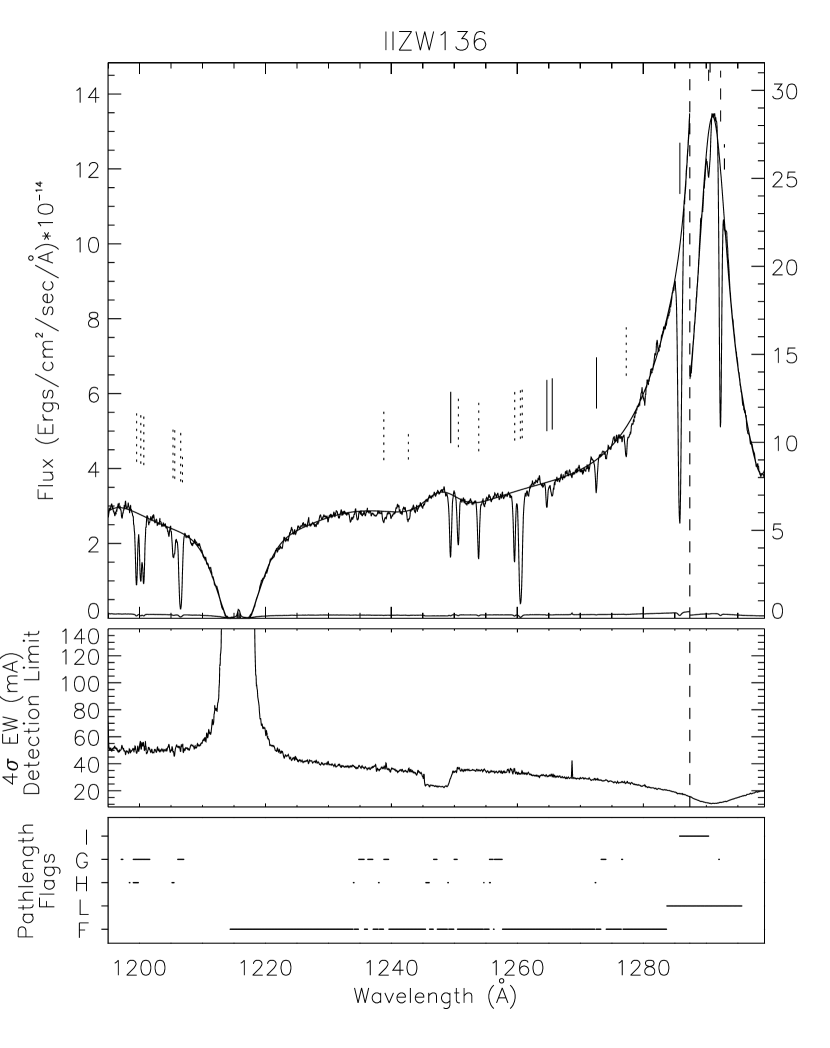
Figure 13: Spectrum, sensitivity limits, and pathlength flags for the II ZW 136 sightline.

The STIS+G140M spectra, error vectors, and pathlength accountings are presented in Figures 12–26 for all targets. The upper panel of each figure presents the composite spectrum and the 1$\sigma$ error values, which are plotted below the flux vector. As discussed in Paper I, our list of intergalactic Ly$\alpha$ absorbers is restricted to those more than 1200 km s^-1 blueward of the target Ly$\alpha$ emission. This limit is indicated by the dashed vertical line in the upper and middle panels of the figures. All non-Galactic features redward of this line are classified as intrinsic absorbers. While we realize that the 1200 km s^-1 limit is somewhat arbitrary, our choice is based upon HST work on intrinsic absorbers by Crenshaw et al. (1999) and is justified in detail in Paper I. All otherwise unidentified absorption features blueward are taken to be intergalactic Ly$\alpha$ absorption features, and are indicated by a solid vertical line above the feature. Ly$\alpha$ absorbers with significance level ($SL$) $>4\sigma\$ are plotted with a solid vertical line. Galactic and high-velocity cloud (HVC) absorption lines are similarly represented with a dotted line ($SL\geq 4\sigma$ longer line, $3\sigma\leq SL<4\sigma$ shorter line), intrinsic absorption lines with a dashed line, and intervening higher-$z$ absorption (Ly$\beta$ and/or O VI) lines with a dot-dashed line. HVCs are identified by their metal absorption lines and have $|cz|\leq 500~{}{\rm km~{}s}^{-1}$. As described in Paper I and § 2, the global continuum fits are a combination of a polynomial of order given in Table 1 for each object plus Gaussian components for Ly$\alpha$ and weaker emission lines from the target and Galactic damped Ly$\alpha$ absorption. The weak emission lines modeled by the continuum fits are described for each target individually in this Appendix. Once the continuum fits are made and the absorption features removed, the remaining continuum fluctuations are Gaussian distributed with a standard deviation equal to the noise vector plotted at the bottom of each spectrum. Given the number of independent REs in our full dataset, we expect that $\sim 10\%$ of the $3\sigma\leq SL<4\sigma$ Ly$\alpha$ absorption features are spurious, but that $\lesssim 0.1\%$ of the $SL\geq 4\sigma$ absorption lines are spurious. However, the specified wavelengths of the Galactic features means that most of the $3\sigma\leq SL<4\sigma$ Galactic absorptions are real. Therefore, we identify all of them and list them in Table 6.

In several cases, where Ly$\alpha$ emission occurs in the observed band, the portion of the spectrum redward of the (c$z_{\rm em}$– 1200 km s^-1) proximity limit (vertical dashed line) is excluded from the region best fitted by the continuum. Thus, any intrinsic or Galactic absorptions redward of the “proximity limit” may not have their rest-frame equivalent widths ($\mathcal{W}$) most accurately represented. The middle panel shows the 4$\sigma$ $\mathcal{W}$ sensitivity detection limit per RE as a function of wavelength for each target. As with the upper panel, we include in our statistics only the portion of the spectrum that lies $>1200$ km s^-1 blueward of the target Ly$\alpha$ emission. Finally, the bottom panel of each figure summarizes the available pathlength for inclusion in our sample and line statistics. The row marked ‘I’ indicates the portion of the spectrum removed due to specific features intrinsic to the target or non-Ly$\alpha$ lines associated with known intervening systems at higher redshift not associated with the target AGN. The pathlength removed due to higher redshift intervening absorbers (PG1116+215 only) is indicated by a double line to differentiate it from that removed due to intrinsic absorption features. The other rows are marked as follows: ‘G’ indicates pathlength attributed to non-HVC Galactic features such as S II $\lambda\lambda$1250.6, 1253.8, 1259.5, ‘H’ indicates pathlength attributed to HVCs, ‘L’ indicates the portion of the spectrum that is redward of c$z_{\rm em}$– 1200 km s^-1 for Ly$\alpha$, and ‘F’ indicates those regions of the spectrum that are available for the detection of intergalactic Ly$\alpha$ absorbers. The ‘F’ row also corrects for our inability to detect and model features near the edge of our wavelength coverage; we remove 10 pixels on the edges of our wavelength coverage. Only for PG 1116+215 (catalog ) does the intrinsic/intervening ‘I’ accounting remove any significant pathlength not already removed by the ‘L’ row. Although not explicitly marked, spectral regions with $\lambda<1218~{}\mbox{\AA}$ are unavailable for the detection of intergalactic Ly$\alpha$ absorbers, owing to Galactic Ly$\alpha$ absorption.

For a few objects, the c$z_{\rm em}$– 1200 km s^-1 “proximity limit” lies within the observed spectral band and is indicated by a dashed vertical line. For targets with strong intrinsic Ly$\alpha$ emission (II ZW 136 (catalog ), MR 2251-178 (catalog ), MRK 926 (catalog ), NGC 985 (catalog ), TON 1542 (catalog ), and TON S180 (catalog )), fluxes are scaled differently above and below this convenient breakpoint. For these spectra, the left axis corresponds to flux blueward of the proximity limit, while the right axis corresponds to flux redward of this limit. In all spectra, the 1$\sigma$ error vector is plotted at the bottom.

The $SL\geq 4\sigma$ line lists for each individual spectrum are presented sequentially in Table 6; Galactic absorptions at $3\sigma\leq SL<4\sigma$ are also listed. The first column of Table 6 indicates the LSR-adjusted wavelength and wavelength uncertainty for each feature. The wavelength scale of each spectrum was corrected to the LSR using the Galactic H I 21 cm emission, N I $\lambda\lambda$1199.5, 1200.2, 1200.7, and S II $\lambda\lambda$1250.6, 1253.8, 1259.5, where available. The second column lists the non-relativistic velocity ($cz$ in km s^-1) relative to the LSR. For Ly$\alpha$ absorbers judged to be intrinsic to the AGN, velocities are listed relative to the AGN narrow-line region (see § 2 and Paper I). For intervening non-Ly$\alpha$ absorbers, we report the velocity ($cz$) of the absorber. We also provide velocity or redshift uncertainties, based upon the total wavelength uncertainties (see § 2 and Paper I). The third column provides the single-component Doppler widths ($b$ in km s^-1) and uncertainties for each feature as estimated from the Gaussian line widths. While the Doppler widths have been corrected for the spectral resolution of STIS, the single-component Gaussian fits were restricted to the range $12<b<100$ km s^-1. However, we neither use nor recommend the use of these derived $b$-values, due both to the complex LSF of the STIS instrument and to an unknown amount of “jitter” during these long exposures (see § 2). The fourth column lists the rest-frame equivalent width ($\mathcal{W}$ in mÅ) and its uncertainty for each absorption feature. This uncertainty includes both the statistical error of the $\chi^{2}$ fit and our conservative estimate of the systematic error in the continuum placement (4.2%). The fifth column indicates the significance level ($SL$  in $\sigma$) of each feature. The $SL$ is calculated by integrating the signal-to-noise ratio (per RE) of the best-fit Gaussian for each feature. The final two columns present the identification (Id) and alternative identification (Alt Id), if applicable for each feature. Absorption lines that are determined not to be intergalactic Ly$\alpha$ have their identifications prefaced by g: (Galactic), h: (HVC), i: (intrinsic), or z: (intervening). Alternate line identifications that lie between 0.2–0.4 Å from the expected location are indicated as speculative by the inclusion of a ? following the identification.

HE 1029-140

The field of this radio-quiet QSO ($z=0.086$) has been studied in detail by Wisotzki (1994) and Bahcall et al. (1997). Surveying a $10\arcmin.2\times 16\arcmin.2$ field, Wisotzki (1994) report a field galaxy, which they designate G10, 4′.2 off the HE 1029-140 (catalog ) line-of-sight at $z=0.0511\pm 0.0002$ ($cz=15,319\pm 60$ km s^-1). This places the galaxy 268$h^{-1}_{70}$ kpc from the sightline with a projected Ly$\alpha$ expected at 1277.8 Å. We report two Ly$\alpha$ features in this region: a weak absorber ($\mathcal{W}=30~{}{\rm m}\mbox{\AA}$) at $cz$=15,369 km s^-1 and a strong absorber ($\mathcal{W}=278~{}{\rm m}\mbox{\AA}$) at $cz=15,464$ km s^-1. Thus, further investigations of the galaxy field at this redshift are warranted. Two HVCs are detected in Si III $\lambda$1206.5 and Si II $\lambda$1260.4 + Fe II $\lambda$1260.5, at velocities of approximately 100 km s^-1 and 200 km s^-1.

Figure 12: STIS spectra, sensitivity limits, and pathlength flags for the HE1029-140 sightline.

II ZW 136

The spectrum of this Seyfert 1 galaxy (also known as UGC 11763 (catalog ), MRK 1513 (catalog ), and PG 2130+099 (catalog )) shows the usual Galactic absorption features plus two HVCs at $-225$ and $-295$ km s^-1. The absorption feature at 1249.4 Å is certainly Ly$\alpha$ and not HVC S II $\lambda$1250, owing to the lack of any absorption associated with S II $\lambda$1253.8 or 1259.5. The Galactic N V $\lambda$1242.8 line is peculiarly strong and asymmetric, indicating possible, but unclaimed blending with extragalactic Ly$\alpha$. The small bump in the continuum near 1248 Å is intrinsic C III $\lambda$1175 emission. Both the shape of the 1285.8 Å Ly$\alpha$ line and its intergalactic/intrinsic nature are uncertain, owing to its proximity to the peak of the AGN Ly$\alpha$ emission.

MR 2251-178

The spectrum of this $z=0.0644$ QSO shows strong intrinsic absorption from $-50$ to $-800$ km s^-1, and HVC gas at $-270$ km s^-1 in Si III $\lambda$1206.5 and Si II $\lambda$1260.4 + Fe II $\lambda$1260.5. The intrinsic absorber also contains Si III $\lambda$1206.5 at two wavelengths: 1282.4 and 1282.7 Å. Far Ultraviolet Spectroscopic Explorer (FUSE) data indicate O VI HVC gas at $-340$ to $-180$ km s^-1 and $-145$ to $-65$ km s^-1 (Sembach et al., 2003). The 9021 km s^-1 absorber is possibly associated with gas in the vicinity of ESO 603-G025 ($cz=9030$ km s^-1, 322$h^{-1}_{70}$ kpc off the line of sight). The strong 3205 km s^-1 absorber is possibly associated with gas in the vicinity of ESO 603-G027 ($cz=3267$ km s^-1, 354$h^{-1}_{70}$ kpc off the line of sight). In fitting the strong intrinsic Ly$\alpha$, our restriction of $b$-value $\leq 100$ km s^-1 (appropriate for the intervening absorbers; see Paper I) results in numerous non-unique components. There is no physical reason to divide the intrinsic absorption like this, but a case can be made for two components: one at 832 km s^-1 and a broad blend of the remaining components.

Figure 14: Spectrum, sensitivity limits, and pathlength flags for the MR 2251-178 sightline.

MRK 478

The spectrum of this Seyfert 1 galaxy shows IVC absorption at $-90$ km s^-1 in Si III $\lambda$1206.5. Asymmetries in the line profiles indicate additional possible IVC absorption in S II $\lambda\lambda$1250.6, 1253.8, 1259.5 and Si II $\lambda$1260.4 + Fe II $\lambda$1260.5. FUSE data indicate O VI HVC gas at 340–435 km s^-1 (Sembach et al., 2003). The continuum bumps at $\sim$1227 Å and 1267 Å are due to intrinsic N I $\lambda$1134.9 and C III $\lambda$1175.7, respectively.

Figure 15: Spectrum, sensitivity limits, and pathlength flags for the MRK 478 sightline.

MRK 926

The spectrum of this QSO shows possible IVC absorption in Si II $\lambda$1260.4 + Fe II $\lambda$1260.5 at $\sim$$-80$ km s^-1. FUSE data indicate O VI HVC gas at $-395$ to $-65$ km s^-1 (Sembach et al., 2003). The spectrum shows extensive intrinsic absorption up to $\sim-1400$ km s^-1 from the recession velocity. In this one case, we have identified the highest relative velocity component in this absorption trough as intrinsic Ly$\alpha$ despite it exceeding the -1200 km s^-1 limit we use to identify probable intrinsic absorbers. We feel that this exception is justified in this case because the component which exceeds -1200 km s^-1 is part of a contiguous absorption trough extending down to $\sim-600$ km s^-1 (see Figure 16 and Table 6). Although the absorption at 1263.19 Å is at approximately the correct wavelength to be intrinsic Si III $\lambda$1206.5, it is much too strong. Therefore, we identify this absorber as intergalactic Ly$\alpha$.

Figure 16: Spectrum, sensitivity limits, and pathlength flags for the MRK 926 sightline.

MRK 1383

The spectrum of this Seyfert 1 galaxy shows an IVC absorption at $\sim$$-45$ km s^-1 in N V $\lambda\lambda$1238.8, 1242.8 and S II $\lambda$1253.8, barely resolved from the Galactic absorption. Asymmetries in the line profiles also suggest possible IVC absorption in Si III $\lambda$1206.5 and Si II $\lambda$1260.4 + Fe II $\lambda$1260.5. FUSE data indicate O VI HVC gas at 100–160 km s^-1 (Sembach et al., 2003). There is a very broad trough (FWHM $\sim$130 km s^-1) of absorption near the location of Galactic C I $\lambda$1280.1 that we identify as extragalactic Ly$\alpha$ due to the absence of Galactic C I $\lambda$1277.2 absorption (see § 2.1 and Table 3). Similarly, we identify the 1250.1 Å feature as Ly$\alpha$ and not HVC S II $\lambda$1250.6 due to the absence of S II $\lambda$1253.8 and S II $\lambda$1259.5 HVC absorption. The continuum bumps near $\sim$1230 Å and 1277 Å, respectively, are intrinsic N I $\lambda$1134.9 and C III $\lambda$1175.7 emission.

Figure 17: Spectrum, sensitivity limits, and pathlength flags for the MRK 1383 sightline.

NGC 985

NGC 985 (MRK 1048) is a composite system of two interacting galaxies with nuclei separated by $\sim$3″, only one of which is an AGN (Appleton & Marcum, 1993). Strong intrinsic absorption systems with velocities relative to NGC 985 between $-200$ and $-800$ km s^-1 are detected in our spectrum in Ly$\alpha$ and N V $\lambda\lambda$1238.8, 1242.8 (Appleton et al., 2002). Bowen et al. (2002) report an association between a Ly$\alpha$ absorber and the galaxy NGC 988 (catalog ) ($cz$=1504 km s^-1, 36.2′ and thus 266$h^{-1}_{70}$ kpc off the line of sight). We do not confirm this Ly$\alpha$ absorber, since our nearest $SL\geq 4\sigma$ Ly$\alpha$ absorber is at 2155 km s^-1. HVC gas at $-230$ to $-110$ km s^-1 is seen in Si III $\lambda$1206.5, S II $\lambda$1253.8, S II $\lambda$1259.5, and Si II $\lambda$1260.4 + Fe II $\lambda$1260.5. The 1238.8 Å ($\mathcal{W}=36\pm 27~{}{\rm m}\mbox{\AA}$) absorption line is identified as Galactic N V $\lambda$1238.8, despite undetected N V $\lambda$1242.8.

Figure 18: Spectrum, sensitivity limits, and pathlength flags for the NGC 985 sightline.

PG 0804+761

The spectrum of this $z$=0.100 QSO contains a strong IVC, seen in most of the Galactic features at $-60$ to $-20$ km s^-1, consistent with Lockman (1999). The accuracy of the central wavelengths and equivalent widths of the blended Galactic N V $\lambda$1238.8 absorption and the corresponding HVC absorption are compromised by the presence of a nearby strong Ly$\alpha$ feature at 1238.2 Å. The continuum bumps at $\sim$1232 Å, 1250 Å, and 1293 Å are intrinsic emission of the C I blend, N I $\lambda$1134.9, and C III $\lambda$1175.7, respectively. Galactic C I $\lambda$1277.2 is particularly strong in this sightline, and the identification is supported by C I $\lambda$1280.1. The broad absorption features near 1222 Å are possibly associated with gas in the neighborhood of UGC 04238 ($cz=1544$ km s^-1, 146$h^{-1}_{70}$ kpc off the line of sight). This is one of the closest Ly$\alpha$ absorber-galaxy associations in our entire survey.

Figure 19: Spectrum, sensitivity limits, and pathlength flags for the PG 0804+8761 sightline.

PG 1116+215

The spectrum of this $z=0.176$ Seyfert 1 shows a strong HVC at 100–215 km s^-1 in Si III $\lambda$1206.5 and Si II $\lambda$1260.4 + Fe II $\lambda$1260.5. The continuum bumps at 1208 Å and 1225 Å are intrinsic Ly$\beta$ and O VI $\lambda\lambda$1031.9, 1037.6 emission, respectively. The 1238–1241 Å spectral region is complicated, with numerous weak absorption features that appear to be a combination of Galactic and HVC N V $\lambda$1238.8 and Mg II $\lambda\lambda$1239.9, 1240.4. Our data support the suspicion of Tripp, Lu, & Savage (1998) that their absorption feature at 5846 km s^-1 is not Ly$\alpha$, but is instead a combination of weak Galactic and HVC absorption. FUSE data indicate O VI HVC gas at 115–310 km s^-1 (Sembach et al., 2003). Intervening Ly$\beta$ absorption is detected at 1196.2 Å ($z$=0.1661), 1197.0 Å ($z$=0.1670), and 1203.9 Å ($z$=0.1736), and intervening O VI $\lambda$1031.9 absorption is seen at $z$=0.1656 and $z$=0.1661, and O VI $\lambda$1037.6 at $z$=0.165 (identifications consistent with Tripp et al. 1998).

Figure 20: Spectrum, sensitivity limits, and pathlength flags for the PG 1116+215 sightline.

PG 1211+143

Lockman (1999) reports $-62$ to +36 km s^-1 IVC gas along the sightline to this $z$=0.0809 Seyfert. We confirm the blueshifted IVC and note two possible HVC absorptions at +180 and +280 km s^-1 in Si III $\lambda$1206.5. The IVCs cause additional uncertainty in the LSR velocity scale. We estimate this additional uncertainty to be $\pm 10$ km s^-1 and have added it in quadrature for all absorptions. The strong absorption systems have been studied by Bowen et al. (2002) and Impey et al. (1999), who discuss potential galaxy associations. The continuum bumps near 1236 Å and 1270 Å are intrinsic N I $\lambda$1134.9 and C III $\lambda$1175.7 emission, respectively. A STIS+E140M spectrum of Ly$\alpha$ and a FUSE spectrum of higher Lyman lines (Tumlinson et al., 2004) confirm the pair of lines near 1268.5 Å as Ly$\alpha$, and not Si III $\lambda$1206.5, related to the Ly$\alpha$ pair at 1278 Å. We identify the absorber at 1284.2 Å as Si III $\lambda$1206.5 associated with the Ly$\alpha$ absorber at 1294 Å.

Figure 21: Spectrum, sensitivity limits, and pathlength flags for the PG 1211+143 sightline.

PG 1351+640

The spectrum of this $z$=0.0882 Seyfert 1 contains evidence for IVC and HVC gas at $\sim$$-50$ and $-150$ km s^-1. The $\sim$$-150$ km s^-1 HVC has previously been reported by Lockman (1999). The $\sim$$-50$ km s^-1 IVC causes additional uncertainty of the LSR velocity scale. We estimate this uncertainty to be $\pm 10$ km s^-1 and have added it in quadrature to the statistical uncertainty for all absorptions. FUSE data indicate O VI HVC gas at $-160$ to $-100$ km s^-1 and 100 to 160 km s^-1 (Sembach et al., 2003). The continuum bumps near 1228 Å and 1280 Å are due to intrinsic N I $\lambda$1134.9 and C III $\lambda$1175.7, respectively. This sightline includes the northwest portion of the Bootes void at $cz$=14,500–17,000 km s^-1 (Kirshner et al., 1987); we detect no Ly$\alpha$ absorbers within this void.

Figure 22: Spectrum, sensitivity limits, and pathlength flags for the PG 1351+640 sightline.

PKS 2005-489

The spectrum of this $z$=0.071 BL Lac object contains strong IVC absorption at 60–90 km s^-1 in N I, N V, Si II, and S II. These IVCs introduce error in the LSR wavelength scale, resulting in higher than average velocity errors. FUSE data indicate O VI HVC gas at 120–225 km s^-1 (Sembach et al., 2003). There is an indication of Galactic and IVC C I $\lambda$1277.2 absorption, but these are not supported by C I $\lambda$1280.2. The continuum bumps near 1228 Å and 1260 Å are intrinsic N I $\lambda$1134.9 and C III $\lambda$1175.7 emission. These weak emissions are the first broad lines detected in this BL Lac object (Falomo et al. (1987) detected narrow H$\alpha$ and [N II] optically). The Galactic N V absorption in this sightline, which is $\sim 30^{\circ}$ above the Galactic center, is the second strongest (after 3C 273) N V observed along any of our sightlines. Higher resolution studies of this sightline are on-going in HST Cycle 12 to probe the outflow associated with the nuclear activity in our own Galaxy.

Figure 23: Spectrum, sensitivity limits, and pathlength flags for the PKS 2005-489 sightline.

TON S180

The spectrum of this $z$=0.06198 Seyfert 1.2 shows HVC gas in Si III $\lambda$1206.5 and Si II $\lambda$1260.4 + Fe II $\lambda$1260.5 at $\sim$$-150$ km s^-1. FUSE data indicate O VI HVC gas at $-265$ to $-100$ km s^-1 and 220 to 280 km s^-1 (Sembach et al., 2003). The continuum bump near 1248 Å is due to intrinsic C III $\lambda$1175.7.

Figure 24: Spectrum, sensitivity limits, and pathlength flags for the TON S180 sightline.

TON 1542

The spectrum of this $z$=0.06301 Seyfert 1 galaxy, also known as MRK 771 and PG 1229+204, does not show any significant HVC absorbers. The 1895 km s^-1 Ly$\alpha$ absorber appears to be associated with the galaxy CGCG 129-006, which lies 20.0′ (160$h^{-1}_{70}$ kpc) off the sightline at 1921 km s^-1. The 1226.0 Å (2536 km s^-1) Ly$\alpha$ absorber appears to be associated with the galaxy NGC4529, which lies 11.4′ (120$h^{-1}_{70}$ kpc) off the line of sight at 2536 km s^-1. It is unclear whether the absorption feature at 1240 Å is Galactic Mg II $\lambda\lambda$1239.9, 1240.4 or Ly$\alpha$. To be conservative, we have identified this absorber as Galactic Mg II. The small spectral continuum bump near 1248 Å is due to intrinsic C III $\lambda$1175.7.

Figure 25: Spectrum, sensitivity limits, and pathlength flags for the TON 1542 sightline.

VII ZW 118

The spectrum of this $z$=0.07966 Seyfert 1 galaxy shows some evidence of IVC gas in Si III $\lambda$1206.5 at $\sim$$-70$ km s^-1, which is consistent with Lockman (1999). This target was observed near the beginning of our program, when the STIS calibration was not as well defined as for later observations. The continuum fit longward of 1230 Å has larger uncertainty than for other objects, owing to the absence of the longer wavelength setting. The continuum bump near 1230 Å is intrinsic N I $\lambda$1134.9. The 2426 and 2469 km s^-1 absorptions are within a galaxy void. No galaxies closer to these absorbers than 3$h^{-1}_{70}$ Mpc have been found, despite considerable efforts to do so (McLin et al., 2002).

Figure 26: Spectrum, sensitivity limits, and pathlength flags for the VII ZW 118 sightline.

Table 6: HST/STIS Absorption Features

Wavelength	Velocity	$b$	$\mathcal{W}$	SL	Id	Alt Id
(Å)	(km s-1)	(km s-1)	(mÅ)	($\sigma$)
HE 1029-140
1199.556 $\pm$ 0.036	2 $\pm$ 9	64 $\pm$ 4	437 $\pm$ 51	36.1	g:NI1199.5	$\cdots$
1200.190 $\pm$ 0.037	-7 $\pm$ 9	47 $\pm$ 6	332 $\pm$ 67	27.6	g:NI1200.2	$\cdots$
1200.686 $\pm$ 0.038	-6 $\pm$ 9	56 $\pm$ 6	374 $\pm$ 67	31.2	g:NI1200.7	$\cdots$
1206.442 $\pm$ 0.041	-14 $\pm$ 10	71 $\pm$ 5	470 $\pm$ 67	39.4	g:SiIII1206.5	$\cdots$
1206.927 $\pm$ 0.039	106 $\pm$ 10	78 $\pm$ 9	478 $\pm$ 103	39.6	h:SiIII1206.5	$\cdots$
1207.332 $\pm$ 0.041	207 $\pm$ 10	$<20$	62 $\pm$ 46	5.1	h:SiIII1206.5	$\cdots$
1223.664 $\pm$ 0.044	1971 $\pm$ 11	53 $\pm$ 10	110 $\pm$ 39	10.1	Ly$\alpha$	$\cdots$
1224.601 $\pm$ 0.041	2202 $\pm$ 10	35 $\pm$ 17	45 $\pm$ 31	4.5	Ly$\alpha$	$\cdots$
1225.496 $\pm$ 0.037	2423 $\pm$ 9	42 $\pm$ 5	183 $\pm$ 32	17.9	Ly$\alpha$	$\cdots$
1234.013 $\pm$ 0.060	4523 $\pm$ 15	52 $\pm$ 19	59 $\pm$ 37	6.4	Ly$\alpha$	$\cdots$
1239.073 $\pm$ 0.050	66 $\pm$ 12	75 $\pm$ 15	109 $\pm$ 41	12.6	g:NV1238.8	$\cdots$
1239.828 $\pm$ 0.048	-23 $\pm$ 12	44 $\pm$ 13	61 $\pm$ 29	7.0	g:MgII1239.9	$\cdots$
1243.099 $\pm$ 0.047	72 $\pm$ 11	64 $\pm$ 12	88 $\pm$ 30	10.6	g:NV1242.8	$\cdots$
1250.562 $\pm$ 0.038	-5 $\pm$ 9	27 $\pm$ 4	148 $\pm$ 26	15.1	g:SII1250.6	$\cdots$
1253.795 $\pm$ 0.038	-4 $\pm$ 9	38 $\pm$ 3	202 $\pm$ 27	22.7	g:SII1253.8	$\cdots$
1259.554 $\pm$ 0.042	13 $\pm$ 10	43 $\pm$ 6	236 $\pm$ 57	24.4	g:SII1259.5	$\cdots$
1260.250 $\pm$ 0.043	179 $\pm$ 10	33 $\pm$ 27	139 $\pm$ 167	14.6	h:SII1259.5	$\cdots$
1260.507 $\pm$ 0.134	2 $\pm$ 9	72 $\pm$ 38	438 $\pm$ 526	46.2	g:SiII+FeII1260.5	$\cdots$
1260.892 $\pm$ 0.042	93 $\pm$ 10	70 $\pm$ 10	352 $\pm$ 108	37.5	h:SiII+FeII1260.5	$\cdots$
1277.173 $\pm$ 0.050	-17 $\pm$ 12	27 $\pm$ 15	59 $\pm$ 39	7.4	g:CI1277.2	Ly$\alpha$
1277.991 $\pm$ 0.042	15369 $\pm$ 10	44 $\pm$ 26	30 $\pm$ 32	4.2	Ly$\alpha$	h:CI1277.2
1278.379 $\pm$ 0.038	15464 $\pm$ 9	42 $\pm$ 3	278 $\pm$ 26	38.0	Ly$\alpha$	$\cdots$
1292.475 $\pm$ 0.049	18941 $\pm$ 12	36 $\pm$ 13	38 $\pm$ 20	5.5	Ly$\alpha$	$\cdots$
1293.352 $\pm$ 0.041	19157 $\pm$ 10	30 $\pm$ 7	62 $\pm$ 18	9.4	Ly$\alpha$	$\cdots$
II ZW 136
1199.545 $\pm$ 0.030	-1 $\pm$ 7	44 $\pm$ 3	302 $\pm$ 37	25.4	g:NI1199.5	$\cdots$
1200.202 $\pm$ 0.030	-5 $\pm$ 8	41 $\pm$ 4	268 $\pm$ 43	22.4	g:NI1200.2	$\cdots$
1200.687 $\pm$ 0.030	-6 $\pm$ 8	41 $\pm$ 5	274 $\pm$ 49	22.7	g:NI1200.7	$\cdots$
1205.313 $\pm$ 0.035	-295 $\pm$ 9	$<20$	66 $\pm$ 37	5.2	h:SiIII1206.5	$\cdots$
1205.593 $\pm$ 0.035	-225 $\pm$ 9	$<20$	63 $\pm$ 39	5.2	h:SiIII1206.5	$\cdots$
1206.533 $\pm$ 0.037	8 $\pm$ 9	65 $\pm$ 10	502 $\pm$ 157	39.9	g:SiIII1206.5
1206.823 $\pm$ 0.035	80 $\pm$ 9	24 $\pm$ 27	46 $\pm$ 55	3.5	h:SiIII1206.5	$\cdots$
1238.783 $\pm$ 0.050	-9 $\pm$ 12	44 $\pm$ 17	47 $\pm$ 29	5.3	g:NV1238.8	h:MgII1239.9
1242.683 $\pm$ 0.036	-29 $\pm$ 9	12 $\pm$ 26	31 $\pm$ 26	3.6	g:NV1242.8	$\cdots$
1249.406 $\pm$ 0.030	8320 $\pm$ 7	33 $\pm$ 4	192 $\pm$ 22	27.2	Ly$\alpha$	$\cdots$
1250.622 $\pm$ 0.031	9 $\pm$ 7	31 $\pm$ 4	150 $\pm$ 23	17.1	g:SII1250.6	$\cdots$
1253.856 $\pm$ 0.031	11 $\pm$ 7	29 $\pm$ 4	180 $\pm$ 24	20.0	g:SII1253.8	$\cdots$
1259.558 $\pm$ 0.031	9 $\pm$ 7	29 $\pm$ 4	206 $\pm$ 24	25.1	g:SII1259.5	$\cdots$
1260.467 $\pm$ 0.034	2 $\pm$ 8	62 $\pm$ 5	471 $\pm$ 74	59.4	g:SiII+FeII1260.5	$\cdots$
1260.759 $\pm$ 0.036	14 $\pm$ 9	25 $\pm$ 8	102 $\pm$ 52	13.0	g:CI1260.7	h:SiII+FeII1260.5
1264.672 $\pm$ 0.036	12084 $\pm$ 9	29 $\pm$ 7	71 $\pm$ 21	9.6	Ly$\alpha$	$\cdots$
1265.522 $\pm$ 0.036	12294 $\pm$ 9	44 $\pm$ 14	52 $\pm$ 27	7.0	Ly$\alpha$	$\cdots$
1272.547 $\pm$ 0.033	14026 $\pm$ 8	27 $\pm$ 6	72 $\pm$ 19	10.4	Ly$\alpha$	$\cdots$
1277.269 $\pm$ 0.036	6 $\pm$ 9	31 $\pm$ 10	57 $\pm$ 24	8.2	g:CI1277.2	Ly$\alpha$
1285.796 $\pm$ 0.031	17293 $\pm$ 7	79 $\pm$ 3	486 $\pm$ 23	105.3	Ly$\alpha$	$\cdots$
1290.345 $\pm$ 0.036	-437 $\pm$ 8	25 $\pm$ 9	22 $\pm$ 9	8.3	i:Ly$\alpha$	$\cdots$
1290.589 $\pm$ 0.037	-381 $\pm$ 9	30 $\pm$ 11	22 $\pm$ 12	8.2	i:Ly$\alpha$	$\cdots$
1292.261 $\pm$ 0.031	7 $\pm$ 7	49 $\pm$ 3	268 $\pm$ 11	95.3	i:Ly$\alpha$	$\cdots$
MR 2251-178
1199.501 $\pm$ 0.039	-12 $\pm$ 10	33 $\pm$ 5	222 $\pm$ 44	14.1	g:NI1199.5	$\cdots$
1200.189 $\pm$ 0.040	-8 $\pm$ 10	32 $\pm$ 7	218 $\pm$ 63	9.6	g:NI1200.2	$\cdots$
1200.672 $\pm$ 0.041	-9 $\pm$ 10	25 $\pm$ 9	189 $\pm$ 70	6.8	g:NI1200.7	$\cdots$
1205.420 $\pm$ 0.039	-268 $\pm$ 10	26 $\pm$ 6	134 $\pm$ 33	11.5	h:SiIII1206.5	$\cdots$
1206.334 $\pm$ 0.042	-41 $\pm$ 11	38 $\pm$ 5	256 $\pm$ 50	21.6	h:SiIII1206.5	$\cdots$
1206.574 $\pm$ 0.042	18 $\pm$ 11	34 $\pm$ 9	215 $\pm$ 74	18.5	g:SiIII1206.5	$\cdots$
1206.809 $\pm$ 0.042	77 $\pm$ 11	35 $\pm$ 7	170 $\pm$ 46	14.9	h:SiIII1206.5	$\cdots$
1224.743 $\pm$ 0.044	2237 $\pm$ 11	$<20$	39 $\pm$ 34	4.1	Ly$\alpha$	$\cdots$
1224.960 $\pm$ 0.058	2291 $\pm$ 14	26 $\pm$ 20	52 $\pm$ 46	5.6	Ly$\alpha$	$\cdots$
1227.978 $\pm$ 0.052	3035 $\pm$ 13	46 $\pm$ 15	60 $\pm$ 32	6.5	Ly$\alpha$	$\cdots$
1228.667 $\pm$ 0.039	3205 $\pm$ 10	69 $\pm$ 4	349 $\pm$ 37	38.7	Ly$\alpha$	$\cdots$
1233.381 $\pm$ 0.043	4368 $\pm$ 11	49 $\pm$ 19	40 $\pm$ 28	4.8	Ly$\alpha$	$\cdots$
1250.605 $\pm$ 0.039	5 $\pm$ 9	$<20$	119 $\pm$ 24	15.2	g:SII1250.6	$\cdots$
1252.249 $\pm$ 0.044	9021 $\pm$ 11	32 $\pm$ 13	51 $\pm$ 28	6.6	Ly$\alpha$	$\cdots$
1253.823 $\pm$ 0.039	3 $\pm$ 9	$<20$	136 $\pm$ 21	17.3	g:SII1253.8	$\cdots$
1255.145 $\pm$ 0.040	9735 $\pm$ 10	43 $\pm$ 3	181 $\pm$ 23	24.0	Ly$\alpha$	$\cdots$
1257.741 $\pm$ 0.044	10375 $\pm$ 11	65 $\pm$ 25	38 $\pm$ 30	5.5	Ly$\alpha$	$\cdots$
1259.391 $\pm$ 0.044	-26 $\pm$ 10	25 $\pm$ 7	76 $\pm$ 24	11.3	h:SII1259.5	$\cdots$
1259.561 $\pm$ 0.044	10 $\pm$ 10	$<20$	124 $\pm$ 22	18.7	g:SII1259.5	$\cdots$
1260.453 $\pm$ 0.040	-11 $\pm$ 9	76 $\pm$ 3	580 $\pm$ 33	89.4	g:SiII+FeII1260.5	$\cdots$
1272.860 $\pm$ 0.044	14103 $\pm$ 11	$<20$	20 $\pm$ 10	4.4	Ly$\alpha$	$\cdots$
1277.276 $\pm$ 0.044	18 $\pm$ 10	$<20$	17 $\pm$ 12	4.1	g:CI1277.2	$\cdots$
1278.801 $\pm$ 0.042	15569 $\pm$ 10	$<20$	17 $\pm$ 8	4.2	Ly$\alpha$	$\cdots$
1280.476 $\pm$ 0.043	15982 $\pm$ 10	26 $\pm$ 7	30 $\pm$ 9	8.2	Ly$\alpha$	i:SiIII1206.5
1282.417 $\pm$ 0.044	16460 $\pm$ 11	30 $\pm$ 17	15 $\pm$ 12	4.5	i:SiIII1206.5	Ly$\alpha$
1282.732 $\pm$ 0.044	16538 $\pm$ 11	$<20$	20 $\pm$ 11	6.1	i:SiIII1206.5	Ly$\alpha$
1290.401 $\pm$ 0.058	-824 $\pm$ 14	97 $\pm$ 3	139 $\pm$ 18	23.3	i:Ly$\alpha$	$\cdots$
1290.934 $\pm$ 0.045	-701 $\pm$ 10	59 $\pm$ 6	287 $\pm$ 61	42.1	i:Ly$\alpha$	$\cdots$
1291.442 $\pm$ 0.045	-583 $\pm$ 10	48 $\pm$ 9	136 $\pm$ 76	20.2	i:Ly$\alpha$	$\cdots$
1291.842 $\pm$ 0.045	-490 $\pm$ 10	71 $\pm$ 22	394 $\pm$ 215	58.6	i:Ly$\alpha$	$\cdots$
1292.085 $\pm$ 0.292	-434 $\pm$ 68	30 $\pm$ 44	41 $\pm$ 50	6.2	i:Ly$\alpha$	$\cdots$
1292.283 $\pm$ 0.817	-388 $\pm$ 189	53 $\pm$ 57	187 $\pm$ 224	27.9	i:Ly$\alpha$	$\cdots$
1292.622 $\pm$ 0.045	-310 $\pm$ 10	78 $\pm$ 77	386 $\pm$ 463	57.8	i:Ly$\alpha$	$\cdots$
1292.942 $\pm$ 0.045	-236 $\pm$ 10	45 $\pm$ 52	30 $\pm$ 37	4.6	i:Ly$\alpha$	$\cdots$
1293.240 $\pm$ 0.430	-167 $\pm$ 100	86 $\pm$ 72	298 $\pm$ 358	45.3	i:Ly$\alpha$	$\cdots$
1293.822 $\pm$ 0.045	-32 $\pm$ 10	75 $\pm$ 41	52 $\pm$ 62	8.0	i:Ly$\alpha$	$\cdots$
1295.407 $\pm$ 0.041	335 $\pm$ 10	48 $\pm$ 5	57 $\pm$ 11	26.0	i:Ly$\alpha$	$\cdots$
MRK 478
1199.121 $\pm$ 0.042	-95 $\pm$ 11	97 $\pm$ 3	49 $\pm$ 19	5.2	h:NI1199.5	$\cdots$
1199.457 $\pm$ 0.038	-23 $\pm$ 10	36 $\pm$ 3	223 $\pm$ 31	24.0	g:NI1199.5	$\cdots$
1200.133 $\pm$ 0.038	-22 $\pm$ 10	39 $\pm$ 3	229 $\pm$ 30	24.9	g:NI1200.2	$\cdots$
1200.637 $\pm$ 0.038	-18 $\pm$ 10	39 $\pm$ 4	202 $\pm$ 29	22.3	g:NI1200.7	$\cdots$
1206.149 $\pm$ 0.042	-87 $\pm$ 11	31 $\pm$ 6	170 $\pm$ 47	20.0	h:SiIII1206.5	$\cdots$
1206.400 $\pm$ 0.039	-25 $\pm$ 10	42 $\pm$ 4	290 $\pm$ 49	33.6	g:SiIII1206.5	$\cdots$
1222.085 $\pm$ 0.040	1582 $\pm$ 10	45 $\pm$ 4	194 $\pm$ 31	22.5	Ly$\alpha$	$\cdots$
1238.547 $\pm$ 0.045	-61 $\pm$ 11	36 $\pm$ 10	55 $\pm$ 23	7.5	h:NV1238.8	$\cdots$
1242.528 $\pm$ 0.076	-66 $\pm$ 18	52 $\pm$ 25	30 $\pm$ 26	3.9	h:NV1242.8	$\cdots$
1250.592 $\pm$ 0.041	2 $\pm$ 10	$<20$	66 $\pm$ 21	8.6	g:SII1250.6	$\cdots$
1251.305 $\pm$ 0.040	8788 $\pm$ 10	58 $\pm$ 3	290 $\pm$ 30	39.3	Ly$\alpha$	$\cdots$
1253.624 $\pm$ 0.044	-66 $\pm$ 10	$<20$	24 $\pm$ 21	3.1	h:SII1253.8	$\cdots$
1253.809 $\pm$ 0.040	-1 $\pm$ 10	$<20$	103 $\pm$ 22	12.8	g:SII1253.8	$\cdots$
1259.229 $\pm$ 0.044	-69 $\pm$ 10	$<20$	25 $\pm$ 22	3.3	h:SII1259.5	$\cdots$
1259.509 $\pm$ 0.040	-2 $\pm$ 10	27 $\pm$ 4	158 $\pm$ 23	20.7	g:SII1259.5	$\cdots$
1260.169 $\pm$ 0.044	-79 $\pm$ 10	38 $\pm$ 3	216 $\pm$ 33	28.3	h:SiII+FeII1260.5	$\cdots$
1260.435 $\pm$ 0.040	-15 $\pm$ 10	41 $\pm$ 3	293 $\pm$ 35	38.2	g:SiII+FeII1260.5	$\cdots$
1295.119 $\pm$ 0.042	19593 $\pm$ 10	43 $\pm$ 6	84 $\pm$ 18	16.2	Ly$\alpha$	$\cdots$
MRK 926
1199.457 $\pm$ 0.051	-11 $\pm$ 12	66 $\pm$ 15	382 $\pm$ 161	8.8	g:NI1199.5	$\cdots$
1200.154 $\pm$ 0.046	-11 $\pm$ 11	36 $\pm$ 13	261 $\pm$ 137	5.6	g:NI1200.2	$\cdots$
1200.655 $\pm$ 0.040	-11 $\pm$ 10	97 $\pm$ 3	342 $\pm$ 77	7.0	g:NI1200.7	$\cdots$
1206.456 $\pm$ 0.046	-11 $\pm$ 11	80 $\pm$ 12	642 $\pm$ 190	13.9	g:SiIII1206.5	$\cdots$
1245.050 $\pm$ 0.051	7245 $\pm$ 12	66 $\pm$ 14	179 $\pm$ 75	9.7	Ly$\alpha$	$\cdots$
1246.068 $\pm$ 0.060	7496 $\pm$ 15	45 $\pm$ 20	72 $\pm$ 53	4.4	Ly$\alpha$	$\cdots$
1250.586 $\pm$ 0.044	1 $\pm$ 10	31 $\pm$ 11	109 $\pm$ 51	5.8	g:SII1250.6	$\cdots$
1253.797 $\pm$ 0.043	-3 $\pm$ 10	50 $\pm$ 9	175 $\pm$ 55	10.3	g:SII1253.8	$\cdots$
1255.108 $\pm$ 0.048	9726 $\pm$ 12	33 $\pm$ 14	77 $\pm$ 44	4.8	Ly$\alpha$	$\cdots$
1256.279 $\pm$ 0.095	10015 $\pm$ 23	73 $\pm$ 34	66 $\pm$ 61	4.4	Ly$\alpha$	$\cdots$
1259.498 $\pm$ 0.038	-5 $\pm$ 9	59 $\pm$ 5	295 $\pm$ 46	24.1	g:SII1259.5	$\cdots$
1260.156 $\pm$ 0.041	-82 $\pm$ 10	32 $\pm$ 13	83 $\pm$ 66	6.9	h:SiII+FeII1260.5	Ly$\alpha$
1260.481 $\pm$ 0.041	-5 $\pm$ 9	66 $\pm$ 6	529 $\pm$ 96	44.3	g:SiII+FeII1260.5	$\cdots$
1263.193 $\pm$ 0.038	11720 $\pm$ 9	22 $\pm$ 5	117 $\pm$ 25	11.4	Ly$\alpha$	i:SiIII1206.5
1267.312 $\pm$ 0.064	-1384 $\pm$ 15	97 $\pm$ 3	122 $\pm$ 16	13.8	i:Ly$\alpha$	$\cdots$
1268.163 $\pm$ 0.078	-1184 $\pm$ 18	97 $\pm$ 3	128 $\pm$ 16	14.6	i:Ly$\alpha$	$\cdots$
1268.993 $\pm$ 0.058	-988 $\pm$ 14	87 $\pm$ 21	131 $\pm$ 62	15.2	i:Ly$\alpha$	$\cdots$
1269.950 $\pm$ 0.051	-763 $\pm$ 12	82 $\pm$ 11	449 $\pm$ 136	54.4	i:Ly$\alpha$	$\cdots$
1270.483 $\pm$ 0.116	-638 $\pm$ 27	62 $\pm$ 26	90 $\pm$ 99	11.4	i:Ly$\alpha$	$\cdots$
1272.722 $\pm$ 0.037	-110 $\pm$ 9	83 $\pm$ 3	596 $\pm$ 32	103.7	i:Ly$\alpha$	$\cdots$
1273.507 $\pm$ 0.037	75 $\pm$ 9	60 $\pm$ 3	453 $\pm$ 29	82.0	i:Ly$\alpha$	$\cdots$
MRK 1383
1196.770 $\pm$ 0.035	-108 $\pm$ 9	52 $\pm$ 34	37 $\pm$ 40	3.5	h:MnII1197.2	$\cdots$
1199.541 $\pm$ 0.030	-2 $\pm$ 8	40 $\pm$ 4	253 $\pm$ 35	26.0	g:NI1199.5	$\cdots$
1200.211 $\pm$ 0.030	-2 $\pm$ 8	35 $\pm$ 3	231 $\pm$ 31	24.3	g:NI1200.2	$\cdots$
1200.684 $\pm$ 0.030	-6 $\pm$ 8	40 $\pm$ 4	233 $\pm$ 34	24.9	g:NI1200.7	$\cdots$
1206.446 $\pm$ 0.031	-14 $\pm$ 8	69 $\pm$ 4	509 $\pm$ 61	50.1	g:SiIII1206.5	$\cdots$
1206.827 $\pm$ 0.036	81 $\pm$ 9	70 $\pm$ 46	42 $\pm$ 50	4.2	h:SiIII1206.5	$\cdots$
1238.615 $\pm$ 0.036	-45 $\pm$ 9	47 $\pm$ 12	74 $\pm$ 32	9.3	h:NV1238.8	$\cdots$
1238.935 $\pm$ 0.036	33 $\pm$ 9	46 $\pm$ 13	66 $\pm$ 30	8.4	g:NV1238.8	$\cdots$
1240.210 $\pm$ 0.128	75 $\pm$ 31	53 $\pm$ 51	24 $\pm$ 29	3.1	g:MgII1239.9	$\cdots$
1242.645 $\pm$ 0.036	-37 $\pm$ 9	30 $\pm$ 15	40 $\pm$ 25	5.1	h:NV1242.8	$\cdots$
1242.885 $\pm$ 0.036	21 $\pm$ 9	$<20$	25 $\pm$ 17	3.1	g:NV1242.8	$\cdots$
1244.438 $\pm$ 0.035	7094 $\pm$ 8	26 $\pm$ 8	54 $\pm$ 19	7.3	Ly$\alpha$	$\cdots$
1245.510 $\pm$ 0.037	7359 $\pm$ 9	31 $\pm$ 10	35 $\pm$ 15	6.8	Ly$\alpha$	$\cdots$
1250.096 $\pm$ 0.033	8490 $\pm$ 8	65 $\pm$ 5	218 $\pm$ 30	30.7	Ly$\alpha$	$\cdots$
1250.614 $\pm$ 0.031	7 $\pm$ 8	$<20$	102 $\pm$ 19	14.1	g:SII1250.6	$\cdots$
1251.968 $\pm$ 0.039	8951 $\pm$ 10	49 $\pm$ 10	66 $\pm$ 22	9.5	Ly$\alpha$	$\cdots$
1253.585 $\pm$ 0.036	-51 $\pm$ 9	30 $\pm$ 20	28 $\pm$ 25	3.8	h:SII1253.8	$\cdots$
1253.845 $\pm$ 0.032	8 $\pm$ 8	28 $\pm$ 4	141 $\pm$ 23	19.5	g:SII1253.8	$\cdots$
1257.200 $\pm$ 0.050	10242 $\pm$ 12	53 $\pm$ 15	54 $\pm$ 27	7.7	Ly$\alpha$	$\cdots$
1259.528 $\pm$ 0.037	2 $\pm$ 9	29 $\pm$ 4	181 $\pm$ 22	24.3	g:SII1259.5	$\cdots$
1260.208 $\pm$ 0.037	-93 $\pm$ 9	34 $\pm$ 5	121 $\pm$ 42	16.2	h:SiII+FeII1260.6	$\cdots$
1260.478 $\pm$ 0.034	4 $\pm$ 8	57 $\pm$ 4	421 $\pm$ 63	56.5	g:SiII+FeII1260.5	$\cdots$
1261.278 $\pm$ 0.037	11247 $\pm$ 9	42 $\pm$ 10	61 $\pm$ 24	8.5	Ly$\alpha$	$\cdots$
1278.793 $\pm$ 0.031	15566 $\pm$ 8	46 $\pm$ 3	282 $\pm$ 20	45.9	Ly$\alpha$	$\cdots$
1280.077 $\pm$ 0.072	15883 $\pm$ 18	27 $\pm$ 34	26 $\pm$ 31	4.2	Ly$\alpha$	g:CI1280.1
1283.147 $\pm$ 0.061	16640 $\pm$ 15	44 $\pm$ 20	25 $\pm$ 20	4.1	Ly$\alpha$	$\cdots$
NGC 985
1199.482 $\pm$ 0.040	-17 $\pm$ 10	46 $\pm$ 4	277 $\pm$ 44	19.1	g:NI1199.5	$\cdots$
1200.189 $\pm$ 0.040	-8 $\pm$ 10	33 $\pm$ 5	218 $\pm$ 41	15.0	g:NI1200.2	$\cdots$
1200.668 $\pm$ 0.040	-10 $\pm$ 10	30 $\pm$ 5	198 $\pm$ 40	13.6	g:NI1200.7	$\cdots$
1205.551 $\pm$ 0.043	-236 $\pm$ 11	24 $\pm$ 21	56 $\pm$ 52	4.0	h:SiIII1206.5	$\cdots$
1206.344 $\pm$ 0.040	-39 $\pm$ 10	61 $\pm$ 4	452 $\pm$ 52	33.2	g:SiIII1206.5	$\cdots$
1206.982 $\pm$ 0.043	120 $\pm$ 11	97 $\pm$ 3	45 $\pm$ 23	3.3	h:SiIII1206.5	$\cdots$
1224.411 $\pm$ 0.078	2156 $\pm$ 19	61 $\pm$ 27	51 $\pm$ 42	4.5	Ly$\alpha$	$\cdots$
1238.805 $\pm$ 0.053	1 $\pm$ 10	28 $\pm$ 17	36 $\pm$ 27	4.0	g:NV1238.8	$\cdots$
1250.596 $\pm$ 0.041	3 $\pm$ 10	$<20$	100 $\pm$ 17	14.6	g:SII1250.6	$\cdots$
1253.324 $\pm$ 0.054	-114 $\pm$ 13	45 $\pm$ 16	38 $\pm$ 22	6.0	h:SII1253.8	Ly$\alpha$
1253.817 $\pm$ 0.041	1 $\pm$ 10	24 $\pm$ 4	120 $\pm$ 17	19.0	g:SII1253.8	$\cdots$
1259.522 $\pm$ 0.041	1 $\pm$ 10	28 $\pm$ 4	154 $\pm$ 16	28.4	g:SII1259.5	$\cdots$
1259.888 $\pm$ 0.045	-145 $\pm$ 11	$<20$	23 $\pm$ 13	4.2	h:SiII+FeII1260.5	h:SII1259.5
1260.398 $\pm$ 0.040	-15 $\pm$ 10	55 $\pm$ 3	426 $\pm$ 22	78.9	g:SiII+FeII1260.5	$\cdots$
1261.020 $\pm$ 0.045	76 $\pm$ 11	38 $\pm$ 21	26 $\pm$ 21	4.8	g:CI1260.7	h:SiII+FeII1260.5
1264.785 $\pm$ 0.045	-788 $\pm$ 11	80 $\pm$ 13	79 $\pm$ 28	16.8	i:Ly$\alpha$	$\cdots$
1265.315 $\pm$ 0.045	-663 $\pm$ 11	63 $\pm$ 4	248 $\pm$ 28	54.9	i:Ly$\alpha$	$\cdots$
1265.813 $\pm$ 0.045	-545 $\pm$ 11	54 $\pm$ 6	183 $\pm$ 62	42.3	i:Ly$\alpha$	$\cdots$
1266.271 $\pm$ 0.048	-437 $\pm$ 11	90 $\pm$ 6	492 $\pm$ 82	118.3	i:Ly$\alpha$	$\cdots$
1267.045 $\pm$ 0.045	-254 $\pm$ 11	94 $\pm$ 3	431 $\pm$ 30	108.9	i:Ly$\alpha$	$\cdots$
1268.576 $\pm$ 0.041	108 $\pm$ 10	38 $\pm$ 3	232 $\pm$ 13	59.1	i:Ly$\alpha$	$\cdots$
1277.242 $\pm$ 0.046	10 $\pm$ 11	$<20$	17 $\pm$ 10	3.7	g:CI1277.2	$\cdots$
1289.358 $\pm$ 0.043	-670 $\pm$ 10	23 $\pm$ 6	63 $\pm$ 17	9.8	i:NV1238.8	$\cdots$
1290.059 $\pm$ 0.046	-507 $\pm$ 11	84 $\pm$ 14	122 $\pm$ 41	19.2	i:NV1238.8	$\cdots$
1290.518 $\pm$ 0.042	-401 $\pm$ 10	35 $\pm$ 3	162 $\pm$ 22	25.6	i:NV1238.8	$\cdots$
1291.067 $\pm$ 0.042	-273 $\pm$ 10	38 $\pm$ 3	150 $\pm$ 19	23.9	i:NV1238.8	$\cdots$
1292.739 $\pm$ 0.042	114 $\pm$ 10	$<20$	100 $\pm$ 15	15.5	i:NV1238.8	$\cdots$
1293.502 $\pm$ 0.047	-674 $\pm$ 11	43 $\pm$ 9	69 $\pm$ 24	10.9	i:NV1242.8	$\cdots$
1294.109 $\pm$ 0.046	-534 $\pm$ 11	56 $\pm$ 15	82 $\pm$ 39	12.8	i:NV1242.8	$\cdots$
1294.638 $\pm$ 0.044	-412 $\pm$ 10	50 $\pm$ 5	156 $\pm$ 30	24.3	i:NV1242.8	$\cdots$
1295.192 $\pm$ 0.043	-283 $\pm$ 10	35 $\pm$ 5	96 $\pm$ 21	14.7	i:NV1242.8	$\cdots$
1296.894 $\pm$ 0.042	110 $\pm$ 10	$<20$	73 $\pm$ 16	11.0	i:NV1242.8	$\cdots$
PG 0804+761
1199.286 $\pm$ 0.045	-53 $\pm$ 11	$<20$	42 $\pm$ 49	5.6	h:NI1199.5	$\cdots$
1199.488 $\pm$ 0.044	-15 $\pm$ 11	45 $\pm$ 6	327 $\pm$ 79	43.4	g:NI1199.5	$\cdots$
1200.137 $\pm$ 0.041	-21 $\pm$ 10	54 $\pm$ 4	375 $\pm$ 43	50.2	g:NI1200.2	$\cdots$
1200.638 $\pm$ 0.041	-18 $\pm$ 10	48 $\pm$ 3	311 $\pm$ 38	41.7	g:NI1200.7	$\cdots$
1205.870 $\pm$ 0.044	-156 $\pm$ 11	$<20$	29 $\pm$ 22	3.8	h:SiIII1206.5	$\cdots$
1206.141 $\pm$ 0.046	-89 $\pm$ 11	39 $\pm$ 7	217 $\pm$ 61	28.1	h:SiIII1206.5	$\cdots$
1206.463 $\pm$ 0.042	-9 $\pm$ 10	52 $\pm$ 3	385 $\pm$ 43	50.2	g:SiIII1206.5	$\cdots$
1220.322 $\pm$ 0.046	1147 $\pm$ 11	38 $\pm$ 4	165 $\pm$ 29	18.9	Ly$\alpha$	$\cdots$
1221.872 $\pm$ 0.048	1530 $\pm$ 12	45 $\pm$ 10	78 $\pm$ 28	10.5	Ly$\alpha$	$\cdots$
1222.242 $\pm$ 0.046	1621 $\pm$ 11	32 $\pm$ 15	41 $\pm$ 27	5.6	Ly$\alpha$	$\cdots$
1238.182 $\pm$ 0.043	5552 $\pm$ 11	50 $\pm$ 4	324 $\pm$ 44	58.5	Ly$\alpha$	$\cdots$
1238.613 $\pm$ 0.047	5658 $\pm$ 11	41 $\pm$ 51	28 $\pm$ 33	5.0	Ly$\alpha$	h:NV1238.8
1239.984 $\pm$ 0.046	20 $\pm$ 11	26 $\pm$ 10	34 $\pm$ 14	6.2	g:MgII1239.9	$\cdots$
1247.624 $\pm$ 0.045	7880 $\pm$ 11	$<20$	18 $\pm$ 9	4.2	Ly$\alpha$	$\cdots$
1250.377 $\pm$ 0.047	-53 $\pm$ 11	$<20$	36 $\pm$ 22	5.0	h:SII1250.6	$\cdots$
1250.625 $\pm$ 0.043	10 $\pm$ 10	29 $\pm$ 4	134 $\pm$ 24	18.8	g:SII1250.6	$\cdots$
1253.644 $\pm$ 0.047	-37 $\pm$ 11	$<20$	68 $\pm$ 20	9.9	h:SII1253.8	$\cdots$
1253.858 $\pm$ 0.043	11 $\pm$ 10	20 $\pm$ 5	154 $\pm$ 20	22.4	g:SII1253.8	$\cdots$
1259.353 $\pm$ 0.047	-35 $\pm$ 11	21 $\pm$ 5	105 $\pm$ 24	15.2	h:SII1259.5	$\cdots$
1259.566 $\pm$ 0.043	16 $\pm$ 10	22 $\pm$ 4	162 $\pm$ 22	23.3	g:SII1259.5	$\cdots$
1260.188 $\pm$ 0.047	-74 $\pm$ 11	41 $\pm$ 4	185 $\pm$ 27	26.5	h:SiII+FeII1260.5	$\cdots$
1260.468 $\pm$ 0.047	2 $\pm$ 11	53 $\pm$ 3	380 $\pm$ 33	54.5	g:SiII+FeII1260.5	$\cdots$
1277.244 $\pm$ 0.047	0 $\pm$ 11	46 $\pm$ 8	77 $\pm$ 22	11.7	g:CI1277.2	$\cdots$
1280.139 $\pm$ 0.048	1 $\pm$ 11	42 $\pm$ 21	26 $\pm$ 21	3.9	g:CI1280.1	$\cdots$
1287.025 $\pm$ 0.048	17597 $\pm$ 12	47 $\pm$ 8	72 $\pm$ 21	12.0	Ly$\alpha$	$\cdots$
1287.681 $\pm$ 0.052	17758 $\pm$ 13	36 $\pm$ 11	38 $\pm$ 18	6.3	Ly$\alpha$	$\cdots$
1289.983 $\pm$ 0.046	18326 $\pm$ 11	$<20$	37 $\pm$ 14	6.1	Ly$\alpha$	$\cdots$
1292.381 $\pm$ 0.048	18918 $\pm$ 12	32 $\pm$ 11	34 $\pm$ 17	5.8	Ly$\alpha$	$\cdots$
PG 1116+215
1196.194 $\pm$ 0.028	49824 $\pm$ 6	34 $\pm$ 6	149 $\pm$ 35	15.1	z:Ly$\beta$	$\cdots$
1197.026 $\pm$ 0.059	50068 $\pm$ 16	41 $\pm$ 21	46 $\pm$ 39	4.4	z:Ly$\beta$	$\cdots$
1199.531 $\pm$ 0.027	-5 $\pm$ 7	45 $\pm$ 4	293 $\pm$ 39	25.1	g:NI1199.5	$\cdots$
1200.201 $\pm$ 0.027	-5 $\pm$ 7	38 $\pm$ 5	277 $\pm$ 57	24.4	g:NI1200.2	$\cdots$
1200.676 $\pm$ 0.028	-8 $\pm$ 7	47 $\pm$ 4	296 $\pm$ 46	26.6	g:NI1200.7	$\cdots$
1202.781 $\pm$ 0.030	49636 $\pm$ 6	40 $\pm$ 7	109 $\pm$ 28	12.1	z:OVI1031.9	$\cdots$
1203.373 $\pm$ 0.033	49817 $\pm$ 7	45 $\pm$ 28	39 $\pm$ 39	3.7	z:OV1031.9	$\cdots$
1203.882 $\pm$ 0.030	52072 $\pm$ 6	38 $\pm$ 7	106 $\pm$ 29	11.8	z:Ly$\beta$	$\cdots$
1206.394 $\pm$ 0.033	-26 $\pm$ 8	22 $\pm$ 28	53 $\pm$ 63	5.4	h:SiIII1206.5	z:OVI1031.9
1206.601 $\pm$ 0.149	25 $\pm$ 26	87 $\pm$ 25	578 $\pm$ 327	58.5	g:SiIII1206.5	$\cdots$
1206.894 $\pm$ 0.033	98 $\pm$ 8	25 $\pm$ 41	63 $\pm$ 76	6.4	h:SiIII1206.5	$\cdots$
1207.308 $\pm$ 0.035	201 $\pm$ 9	41 $\pm$ 6	227 $\pm$ 75	22.8	h:SiIII1206.5	$\cdots$
1209.403 $\pm$ 0.034	49633 $\pm$ 8	46 $\pm$ 10	76 $\pm$ 27	9.1	z:OVI1037.6	$\cdots$
1221.749 $\pm$ 0.038	1499 $\pm$ 9	52 $\pm$ 12	82 $\pm$ 33	8.6	Ly$\alpha$	$\cdots$
1235.594 $\pm$ 0.032	4913 $\pm$ 8	30 $\pm$ 9	90 $\pm$ 32	9.4	Ly$\alpha$	$\cdots$
1250.212 $\pm$ 0.033	8518 $\pm$ 8	45 $\pm$ 4	227 $\pm$ 32	27.2	Ly$\alpha$	$\cdots$
1250.575 $\pm$ 0.033	-6 $\pm$ 8	$<20$	80 $\pm$ 30	9.1	g:SII1250.6	$\cdots$
1250.724 $\pm$ 0.033	30 $\pm$ 8	$<20$	27 $\pm$ 21	3.0	h:SII1250.6	$\cdots$
1253.799 $\pm$ 0.033	0 $\pm$ 7	22 $\pm$ 5	115 $\pm$ 27	14.1	g:SII1253.8	$\cdots$
1253.949 $\pm$ 0.033	36 $\pm$ 8	42 $\pm$ 11	68 $\pm$ 33	8.2	h:SII1253.8	$\cdots$
1254.799 $\pm$ 0.033	239 $\pm$ 8	58 $\pm$ 24	48 $\pm$ 40	6.0	h:SII1253.8	$\cdots$
1254.989 $\pm$ 0.033	9696 $\pm$ 8	25 $\pm$ 11	68 $\pm$ 34	8.8	Ly$\alpha$	$\cdots$
1259.525 $\pm$ 0.028	6 $\pm$ 7	25 $\pm$ 4	180 $\pm$ 30	21.3	g:SII1259.5	$\cdots$
1260.415 $\pm$ 0.034	-20 $\pm$ 8	47 $\pm$ 3	378 $\pm$ 36	44.4	g:SiII+FeII1260.5	$\cdots$
1260.730 $\pm$ 0.049	55 $\pm$ 12	36 $\pm$ 11	224 $\pm$ 257	26.2	h:SiII+FeII1260.5	g:CII1260.7
1261.085 $\pm$ 0.034	139 $\pm$ 8	64 $\pm$ 66	65 $\pm$ 78	7.6	h:SiII+FeII1260.5	Ly$\alpha$
1261.355 $\pm$ 0.034	203 $\pm$ 8	$<20$	144 $\pm$ 173	16.9	h:SiII+FeII1260.5	$\cdots$
1261.585 $\pm$ 0.034	258 $\pm$ 8	$<20$	43 $\pm$ 51	5.0	h:SiII+FeII1260.5	Ly$\alpha$
1265.780 $\pm$ 0.122	12357 $\pm$ 30	89 $\pm$ 39	88 $\pm$ 82	10.6	Ly$\alpha$	$\cdots$
1266.474 $\pm$ 0.206	12529 $\pm$ 51	80 $\pm$ 55	44 $\pm$ 53	5.4	Ly$\alpha$	$\cdots$
1269.606 $\pm$ 0.065	13301 $\pm$ 16	83 $\pm$ 22	65 $\pm$ 34	8.3	Ly$\alpha$	$\cdots$
1287.438 $\pm$ 0.031	17698 $\pm$ 7	51 $\pm$ 6	167 $\pm$ 31	20.0	Ly$\alpha$	$\cdots$
1289.583 $\pm$ 0.036	18227 $\pm$ 9	38 $\pm$ 9	77 $\pm$ 28	8.9	Ly$\alpha$	$\cdots$
1291.754 $\pm$ 0.067	18763 $\pm$ 16	57 $\pm$ 23	42 $\pm$ 31	4.8	Ly$\alpha$	$\cdots$
PG 1211+143
1199.499 $\pm$ 0.052	-13 $\pm$ 16	43 $\pm$ 4	263 $\pm$ 37	22.3	g:NI1199.5	$\cdots$
1200.160 $\pm$ 0.053	-15 $\pm$ 17	46 $\pm$ 5	252 $\pm$ 46	21.7	g:NI1200.2	$\cdots$
1200.646 $\pm$ 0.053	-16 $\pm$ 17	41 $\pm$ 5	240 $\pm$ 43	20.9	g:NI1200.7	$\cdots$
1206.422 $\pm$ 0.055	-19 $\pm$ 17	50 $\pm$ 6	241 $\pm$ 58	21.5	h:SiIII1206.5	$\cdots$
1206.612 $\pm$ 0.055	28 $\pm$ 17	65 $\pm$ 9	239 $\pm$ 75	21.4	g:SiIII1206.5	$\cdots$
1207.212 $\pm$ 0.055	177 $\pm$ 17	$<20$	45 $\pm$ 28	4.1	h:SiIII1206.5	$\cdots$
1207.627 $\pm$ 0.055	280 $\pm$ 17	25 $\pm$ 18	40 $\pm$ 31	3.6	h:SiIII1206.5	$\cdots$
1224.305 $\pm$ 0.060	2130 $\pm$ 18	97 $\pm$ 3	186 $\pm$ 19	19.1	Ly$\alpha$	$\cdots$
1235.718 $\pm$ 0.057	4944 $\pm$ 17	58 $\pm$ 7	189 $\pm$ 46	21.1	Ly$\alpha$	$\cdots$
1236.093 $\pm$ 0.057	5036 $\pm$ 17	34 $\pm$ 6	154 $\pm$ 40	17.6	Ly$\alpha$	$\cdots$
1239.146 $\pm$ 0.057	84 $\pm$ 17	30 $\pm$ 14	42 $\pm$ 25	4.8	h:NV1238.8	Ly$\alpha$
1239.886 $\pm$ 0.057	-3 $\pm$ 16	37 $\pm$ 16	52 $\pm$ 33	5.9	g:MgII1239.9	$\cdots$
1242.492 $\pm$ 0.062	6615 $\pm$ 18	32 $\pm$ 13	89 $\pm$ 54	10.9	Ly$\alpha$	$\cdots$
1242.826 $\pm$ 0.057	5 $\pm$ 17	49 $\pm$ 56	28 $\pm$ 33	3.3	g:NV1242.8	$\cdots$
1244.064 $\pm$ 0.055	7002 $\pm$ 17	54 $\pm$ 6	150 $\pm$ 30	17.7	Ly$\alpha$	$\cdots$
1247.106 $\pm$ 0.056	7752 $\pm$ 17	75 $\pm$ 6	159 $\pm$ 26	25.7	Ly$\alpha$	$\cdots$
1250.578 $\pm$ 0.062	-5 $\pm$ 16	28 $\pm$ 12	119 $\pm$ 73	13.3	g:SII1250.6	$\cdots$
1253.714 $\pm$ 0.057	-21 $\pm$ 17	$<20$	59 $\pm$ 39	6.5	h:SII1253.8	$\cdots$
1253.867 $\pm$ 0.058	13 $\pm$ 17	23 $\pm$ 9	124 $\pm$ 54	14.1	g:SII1253.8	$\cdots$
1259.444 $\pm$ 0.058	-13 $\pm$ 17	$<20$	101 $\pm$ 55	11.7	h:SII1259.5	$\cdots$
1259.593 $\pm$ 0.058	22 $\pm$ 17	$<20$	99 $\pm$ 94	11.2	g:SII1259.5	$\cdots$
1260.349 $\pm$ 0.058	-36 $\pm$ 17	34 $\pm$ 15	204 $\pm$ 209	23.2	h:SiII+FeII1260.5	$\cdots$
1260.589 $\pm$ 0.058	21 $\pm$ 17	35 $\pm$ 4	238 $\pm$ 65	27.5	g:SiII+FeII1260.5	$\cdots$
1261.249 $\pm$ 0.058	178 $\pm$ 17	$<20$	31 $\pm$ 19	3.7	h:SiII+FeII1260.5	Ly$\alpha$
1268.428 $\pm$ 0.058	13010 $\pm$ 17	54 $\pm$ 8	216 $\pm$ 56	29.3	Ly$\alpha$	z:SiIII1206.5
1268.662 $\pm$ 0.057	13068 $\pm$ 17	31 $\pm$ 7	95 $\pm$ 30	13.0	Ly$\alpha$	z:SiIII1206.5
1270.625 $\pm$ 0.056	13552 $\pm$ 17	$<20$	44 $\pm$ 17	5.9	Ly$\alpha$	$\cdots$
1277.318 $\pm$ 0.058	28 $\pm$ 17	28 $\pm$ 12	51 $\pm$ 30	6.4	g:CI1277.2	$\cdots$
1277.718 $\pm$ 0.056	15301 $\pm$ 17	55 $\pm$ 5	308 $\pm$ 54	40.5	Ly$\alpha$	$\cdots$
1278.221 $\pm$ 0.057	15426 $\pm$ 17	97 $\pm$ 3	691 $\pm$ 25	90.6	Ly$\alpha$	$\cdots$
1278.948 $\pm$ 0.058	15605 $\pm$ 17	42 $\pm$ 5	132 $\pm$ 28	17.2	Ly$\alpha$	$\cdots$
1281.838 $\pm$ 0.058	16318 $\pm$ 17	54 $\pm$ 28	51 $\pm$ 49	7.2	Ly$\alpha$	$\cdots$
1284.209 $\pm$ 0.059	16902 $\pm$ 17	61 $\pm$ 19	57 $\pm$ 34	8.3	z:SiIII1206.5	Ly$\alpha$
1294.047 $\pm$ 0.059	19328 $\pm$ 18	74 $\pm$ 3	564 $\pm$ 31	92.4	Ly$\alpha$	$\cdots$
1294.612 $\pm$ 0.059	19468 $\pm$ 18	56 $\pm$ 3	249 $\pm$ 26	41.7	Ly$\alpha$	$\cdots$
1295.167 $\pm$ 0.059	19604 $\pm$ 18	60 $\pm$ 12	67 $\pm$ 25	11.4	Ly$\alpha$	$\cdots$
PG 1351+640
1198.910 $\pm$ 0.039	-147 $\pm$ 14	91 $\pm$ 14	283 $\pm$ 86	18.3	h:NI1199.5	$\cdots$
1199.405 $\pm$ 0.040	-24 $\pm$ 14	66 $\pm$ 9	450 $\pm$ 119	28.7	g:NI1199.5	$\cdots$
1200.046 $\pm$ 0.049	-38 $\pm$ 16	70 $\pm$ 18	493 $\pm$ 261	30.9	g:NI1200.2	$\cdots$
1200.547 $\pm$ 0.055	-38 $\pm$ 17	61 $\pm$ 11	405 $\pm$ 171	25.0	g:NI1200.7	$\cdots$
1205.903 $\pm$ 0.039	-148 $\pm$ 14	45 $\pm$ 6	292 $\pm$ 62	19.0	h:SiIII1206.5	$\cdots$
1206.153 $\pm$ 0.039	-86 $\pm$ 14	20 $\pm$ 11	101 $\pm$ 50	6.4	h:SiIII1206.5	$\cdots$
1206.454 $\pm$ 0.039	-12 $\pm$ 14	73 $\pm$ 6	545 $\pm$ 88	33.2	g:SiIII1206.5	$\cdots$
1246.677 $\pm$ 0.036	7647 $\pm$ 13	$<20$	34 $\pm$ 15	4.3	Ly$\alpha$	$\cdots$
1250.372 $\pm$ 0.039	-55 $\pm$ 14	$<20$	80 $\pm$ 37	6.4	h:SII1250.6	$\cdots$
1250.570 $\pm$ 0.040	-7 $\pm$ 13	43 $\pm$ 13	109 $\pm$ 54	8.5	g:SII1250.6	$\cdots$
1253.582 $\pm$ 0.037	-52 $\pm$ 13	23 $\pm$ 6	156 $\pm$ 40	12.2	h:SII1253.8	$\cdots$
1253.810 $\pm$ 0.040	2 $\pm$ 13	$<20$	113 $\pm$ 38	8.8	g:SII1253.8	$\cdots$
1259.279 $\pm$ 0.040	-53 $\pm$ 14	$<20$	48 $\pm$ 47	3.6	h:SII1259.5	$\cdots$
1259.559 $\pm$ 0.040	14 $\pm$ 14	88 $\pm$ 16	533 $\pm$ 222	41.1	g:SII1259.5	$\cdots$
1260.019 $\pm$ 0.040	-114 $\pm$ 14	69 $\pm$ 15	389 $\pm$ 185	30.3	h:SiII+FeII1260.5	$\cdots$
1260.269 $\pm$ 0.040	-55 $\pm$ 14	44 $\pm$ 32	95 $\pm$ 114	7.4	h:SiII+FeII1260.5	$\cdots$
1260.509 $\pm$ 0.040	2 $\pm$ 13	59 $\pm$ 7	353 $\pm$ 84	27.7	g:SiII+FeII1260.5	$\cdots$
1276.878 $\pm$ 0.041	-755 $\pm$ 14	54 $\pm$ 24	50 $\pm$ 39	4.6	h:CI1280.1	Ly$\alpha$
1277.298 $\pm$ 0.041	23 $\pm$ 14	$<20$	35 $\pm$ 22	3.4	g:CI1277.2	$\cdots$
1280.278 $\pm$ 0.041	42 $\pm$ 14	43 $\pm$ 24	33 $\pm$ 31	3.5	g:CI1280.1	$\cdots$
1297.287 $\pm$ 0.039	20127 $\pm$ 14	$<20$	42 $\pm$ 18	5.1	Ly$\alpha$	$\cdots$
PKS 2005-489
1197.140 $\pm$ 0.053	-15 $\pm$ 13	55 $\pm$ 14	47 $\pm$ 22	7.8	g:MnII1197.2	$\cdots$
1198.868 $\pm$ 0.053	-158 $\pm$ 13	41 $\pm$ 33	19 $\pm$ 23	3.3	h:NI1199.5	$\cdots$
1199.451 $\pm$ 0.054	-12 $\pm$ 13	58 $\pm$ 6	375 $\pm$ 85	62.8	g:NI1199.5	$\cdots$
1199.802 $\pm$ 0.056	-99 $\pm$ 14	36 $\pm$ 16	137 $\pm$ 118	22.9	h:NI1200.2	h:NI1199.5
1200.116 $\pm$ 0.053	-26 $\pm$ 13	37 $\pm$ 9	226 $\pm$ 98	37.7	g:NI1200.2	$\cdots$
1200.572 $\pm$ 0.051	-34 $\pm$ 13	75 $\pm$ 6	458 $\pm$ 77	75.8	g:NI1200.7	$\cdots$
1201.060 $\pm$ 0.053	87 $\pm$ 13	38 $\pm$ 13	40 $\pm$ 25	6.6	h:NI1200.7	$\cdots$
1206.254 $\pm$ 0.053	-61 $\pm$ 13	43 $\pm$ 3	221 $\pm$ 43	37.1	h:SiIII1206.5	$\cdots$
1206.554 $\pm$ 0.053	13 $\pm$ 13	57 $\pm$ 12	356 $\pm$ 126	60.0	g:SiIII1206.5	$\cdots$
1206.818 $\pm$ 0.051	79 $\pm$ 13	45 $\pm$ 9	177 $\pm$ 59	30.0	h:SiIII1206.5	$\cdots$
1207.124 $\pm$ 0.053	155 $\pm$ 13	22 $\pm$ 14	35 $\pm$ 26	6.0	h:SiIII1206.5	$\cdots$
1226.831 $\pm$ 0.061	2752 $\pm$ 15	31 $\pm$ 15	24 $\pm$ 15	5.1	Ly$\alpha$	$\cdots$
1235.730 $\pm$ 0.051	4947 $\pm$ 13	59 $\pm$ 3	299 $\pm$ 26	68.1	Ly$\alpha$	$\cdots$
1236.192 $\pm$ 0.051	5061 $\pm$ 12	40 $\pm$ 3	281 $\pm$ 21	64.1	Ly$\alpha$	$\cdots$
1238.763 $\pm$ 0.054	-9 $\pm$ 12	70 $\pm$ 10	105 $\pm$ 30	23.5	g:NV1238.8	$\cdots$
1239.073 $\pm$ 0.054	66 $\pm$ 13	46 $\pm$ 8	87 $\pm$ 26	19.5	h:NV1238.8	$\cdots$
1239.673 $\pm$ 0.054	-61 $\pm$ 13	58 $\pm$ 60	19 $\pm$ 23	4.4	h:MgII1239.9	$\cdots$
1239.863 $\pm$ 0.054	-15 $\pm$ 13	$<20$	16 $\pm$ 19	3.6	g:MgII1239.9	$\cdots$
1240.254 $\pm$ 0.055	86 $\pm$ 13	40 $\pm$ 50	16 $\pm$ 19	3.6	h:MgII1239.9	$\cdots$
1242.717 $\pm$ 0.055	-20 $\pm$ 13	45 $\pm$ 50	33 $\pm$ 40	7.4	g:NV1242.8	$\cdots$
1243.002 $\pm$ 0.056	49 $\pm$ 14	35 $\pm$ 7	56 $\pm$ 25	12.7	h:NV1242.8	$\cdots$
1246.445 $\pm$ 0.055	7589 $\pm$ 13	47 $\pm$ 23	14 $\pm$ 11	4.5	Ly$\alpha$	$\cdots$
1250.316 $\pm$ 0.055	-68 $\pm$ 13	$<20$	20 $\pm$ 15	4.3	h:SII1250.6	$\cdots$
1250.564 $\pm$ 0.052	-5 $\pm$ 13	$<20$	105 $\pm$ 30	22.9	g:SII1250.6	$\cdots$
1250.821 $\pm$ 0.063	53 $\pm$ 15	36 $\pm$ 11	71 $\pm$ 37	15.8	h:SII1250.6	$\cdots$
1253.603 $\pm$ 0.055	-1404 $\pm$ 13	41 $\pm$ 13	40 $\pm$ 21	8.7	h:SII1259.5	$\cdots$
1253.798 $\pm$ 0.052	-24 $\pm$ 12	20 $\pm$ 4	131 $\pm$ 29	28.6	g:SII1253.8	$\cdots$
1254.088 $\pm$ 0.055	-66 $\pm$ 13	36 $\pm$ 7	100 $\pm$ 31	21.6	h:SII1259.5	$\cdots$
1259.311 $\pm$ 0.055	-45 $\pm$ 13	28 $\pm$ 44	33 $\pm$ 40	7.4	h:SII1259.5	$\cdots$
1259.512 $\pm$ 0.092	3 $\pm$ 12	28 $\pm$ 11	178 $\pm$ 200	40.2	g:SII1259.5	$\cdots$
1259.788 $\pm$ 0.053	64 $\pm$ 13	21 $\pm$ 6	104 $\pm$ 34	23.6	h:SII1259.5	$\cdots$
1260.310 $\pm$ 0.055	-45 $\pm$ 13	56 $\pm$ 5	417 $\pm$ 79	95.9	g:SiII+FeII1260.5	$\cdots$
1260.704 $\pm$ 0.054	49 $\pm$ 13	50 $\pm$ 4	365 $\pm$ 72	84.7	h:SiII+FeII1260.5	g:CI1260.7
1261.131 $\pm$ 0.055	150 $\pm$ 13	$<20$	29 $\pm$ 17	6.7	h:SiII+FeII1260.5	h:CI1260.7
1266.740 $\pm$ 0.065	12594 $\pm$ 16	44 $\pm$ 16	22 $\pm$ 13	5.3	Ly$\alpha$	$\cdots$
1273.763 $\pm$ 0.054	14326 $\pm$ 13	39 $\pm$ 7	49 $\pm$ 13	11.8	Ly$\alpha$	$\cdots$
1277.114 $\pm$ 0.064	-20 $\pm$ 15	48 $\pm$ 15	32 $\pm$ 17	7.5	g:CI1277.2	$\cdots$
1277.572 $\pm$ 0.057	15265 $\pm$ 14	25 $\pm$ 10	27 $\pm$ 12	6.6	Ly$\alpha$	h:CII1277.2
1285.845 $\pm$ 0.053	17306 $\pm$ 13	47 $\pm$ 3	294 $\pm$ 15	72.7	Ly$\alpha$	$\cdots$
1294.654 $\pm$ 0.053	19478 $\pm$ 13	37 $\pm$ 3	249 $\pm$ 15	63.3	Ly$\alpha$	$\cdots$
1295.191 $\pm$ 0.057	-107 $\pm$ 13	97 $\pm$ 3	30 $\pm$ 19	7.0	g:SI1295.7?	$\cdots$
TON S180
1199.481 $\pm$ 0.043	-17 $\pm$ 11	52 $\pm$ 5	229 $\pm$ 34	21.5	g:NI1199.5	$\cdots$
1200.140 $\pm$ 0.043	-20 $\pm$ 11	18 $\pm$ 5	152 $\pm$ 26	14.1	g:NI1200.2	$\cdots$
1200.614 $\pm$ 0.044	-24 $\pm$ 11	45 $\pm$ 5	185 $\pm$ 35	17.0	g:NI1200.7	$\cdots$
1205.843 $\pm$ 0.044	-163 $\pm$ 11	53 $\pm$ 5	287 $\pm$ 43	26.1	h:SiIII1206.5	$\cdots$
1206.457 $\pm$ 0.043	-11 $\pm$ 11	57 $\pm$ 3	415 $\pm$ 45	38.2	g:SiIII1206.5	$\cdots$
1223.452 $\pm$ 0.049	1919 $\pm$ 12	35 $\pm$ 11	66 $\pm$ 28	6.5	Ly$\alpha$	$\cdots$
1226.921 $\pm$ 0.051	2774 $\pm$ 12	28 $\pm$ 13	49 $\pm$ 26	4.9	Ly$\alpha$	$\cdots$
1227.774 $\pm$ 0.049	2985 $\pm$ 12	21 $\pm$ 13	41 $\pm$ 23	4.3	Ly$\alpha$	$\cdots$
1237.982 $\pm$ 0.046	5502 $\pm$ 11	51 $\pm$ 5	268 $\pm$ 54	31.2	Ly$\alpha$	$\cdots$
1241.177 $\pm$ 0.048	6290 $\pm$ 12	28 $\pm$ 10	54 $\pm$ 23	6.2	Ly$\alpha$	$\cdots$
1244.125 $\pm$ 0.045	7017 $\pm$ 11	56 $\pm$ 4	222 $\pm$ 29	30.0	Ly$\alpha$	$\cdots$
1250.592 $\pm$ 0.046	2 $\pm$ 11	33 $\pm$ 7	87 $\pm$ 25	9.8	g:SII1250.6	$\cdots$
1253.591 $\pm$ 0.048	-50 $\pm$ 12	39 $\pm$ 22	41 $\pm$ 36	4.5	h:SII1253.8	$\cdots$
1253.798 $\pm$ 0.045	-3 $\pm$ 11	$<20$	83 $\pm$ 28	9.1	g:SII1253.8	$\cdots$
1257.901 $\pm$ 0.052	10415 $\pm$ 13	30 $\pm$ 13	41 $\pm$ 23	5.0	Ly$\alpha$	$\cdots$
1259.506 $\pm$ 0.045	-3 $\pm$ 11	$<20$	124 $\pm$ 21	14.9	g:SII1259.5	$\cdots$
1259.816 $\pm$ 0.047	-153 $\pm$ 11	$<20$	30 $\pm$ 17	3.5	h:SiII+FeII1260.5	$\cdots$
1260.409 $\pm$ 0.044	-12 $\pm$ 11	51 $\pm$ 3	384 $\pm$ 33	45.1	g:SiII+FeII1260.5	$\cdots$
1268.027 $\pm$ 0.049	12912 $\pm$ 12	81 $\pm$ 15	107 $\pm$ 39	14.3	Ly$\alpha$	$\cdots$
1268.661 $\pm$ 0.047	13068 $\pm$ 12	52 $\pm$ 5	140 $\pm$ 27	18.7	Ly$\alpha$	$\cdots$
1270.473 $\pm$ 0.048	13515 $\pm$ 12	58 $\pm$ 7	140 $\pm$ 29	19.0	Ly$\alpha$	$\cdots$
1271.147 $\pm$ 0.046	13681 $\pm$ 11	54 $\pm$ 4	212 $\pm$ 29	28.1	Ly$\alpha$	$\cdots$
1290.376 $\pm$ 0.048	-149 $\pm$ 11	42 $\pm$ 6	74 $\pm$ 20	19.9	i:Ly$\alpha$	$\cdots$
1290.960 $\pm$ 0.046	-13 $\pm$ 11	$<20$	39 $\pm$ 14	10.6	i:Ly$\alpha$	$\cdots$
1291.414 $\pm$ 0.045	92 $\pm$ 11	24 $\pm$ 4	107 $\pm$ 14	27.9	i:Ly$\alpha$	$\cdots$
TON 1542
1199.520 $\pm$ 0.032	5 $\pm$ 8	40 $\pm$ 4	244 $\pm$ 41	17.6	g:NI1199.5	$\cdots$
1200.172 $\pm$ 0.032	-7 $\pm$ 8	30 $\pm$ 4	237 $\pm$ 40	16.8	g:NI1200.2	$\cdots$
1200.671 $\pm$ 0.033	-7 $\pm$ 8	43 $\pm$ 5	270 $\pm$ 48	18.8	g:NI1200.7	$\cdots$
1206.287 $\pm$ 0.037	-53 $\pm$ 9	$<20$	69 $\pm$ 82	4.8	h:SiIII1206.5	$\cdots$
1206.479 $\pm$ 0.086	-5 $\pm$ 8	44 $\pm$ 53	290 $\pm$ 347	20.5	g:SiIII1206.5	$\cdots$
1206.707 $\pm$ 0.037	52 $\pm$ 9	27 $\pm$ 9	124 $\pm$ 148	8.9	h:SiIII1206.5	$\cdots$
1220.480 $\pm$ 0.033	1186 $\pm$ 8	47 $\pm$ 5	294 $\pm$ 56	19.7	Ly$\alpha$	$\cdots$
1223.355 $\pm$ 0.033	1895 $\pm$ 8	35 $\pm$ 5	216 $\pm$ 42	16.9	Ly$\alpha$	$\cdots$
1226.063 $\pm$ 0.033	2563 $\pm$ 8	49 $\pm$ 5	248 $\pm$ 41	19.6	Ly$\alpha$	$\cdots$
1238.882 $\pm$ 0.057	15 $\pm$ 14	46 $\pm$ 19	50 $\pm$ 35	4.6	g:NV1238.8	$\cdots$
1240.014 $\pm$ 0.061	22 $\pm$ 15	69 $\pm$ 20	76 $\pm$ 42	6.7	g:MgII1239.9	$\cdots$
1242.902 $\pm$ 0.061	24 $\pm$ 15	50 $\pm$ 21	50 $\pm$ 36	4.7	g:NV1242.8	$\cdots$
1250.607 $\pm$ 0.035	5 $\pm$ 8	$<20$	80 $\pm$ 29	6.9	g:SII1250.6	$\cdots$
1253.832 $\pm$ 0.034	5 $\pm$ 8	$<20$	124 $\pm$ 31	10.7	g:SII1253.8	$\cdots$
1259.540 $\pm$ 0.041	5 $\pm$ 10	32 $\pm$ 9	158 $\pm$ 65	13.7	g:SII1259.5	$\cdots$
1260.478 $\pm$ 0.033	-5 $\pm$ 8	57 $\pm$ 3	444 $\pm$ 39	40.3	g:SiII+FeII1260.5	$\cdots$
1282.406 $\pm$ 0.034	16458 $\pm$ 8	31 $\pm$ 4	105 $\pm$ 20	15.0	Ly$\alpha$	$\cdots$
1289.496 $\pm$ 0.034	-644 $\pm$ 8	$<20$	54 $\pm$ 11	11.1	i:Ly$\alpha$	$\cdots$
VII ZW 118
1197.440 $\pm$ 0.029	60 $\pm$ 7	97 $\pm$ 3	34 $\pm$ 17	3.5	h:MnII1197.2?	$\cdots$
1199.544 $\pm$ 0.022	-1 $\pm$ 6	42 $\pm$ 3	289 $\pm$ 28	30.8	g:NI1199.5	$\cdots$
1200.227 $\pm$ 0.022	2 $\pm$ 6	42 $\pm$ 3	271 $\pm$ 32	28.5	g:NI1200.2	$\cdots$
1200.712 $\pm$ 0.022	0 $\pm$ 6	33 $\pm$ 4	236 $\pm$ 31	24.6	g:NI1200.7	$\cdots$
1201.127 $\pm$ 0.029	107 $\pm$ 7	$<20$	31 $\pm$ 27	3.2	h:NI1200.7	$\cdots$
1206.204 $\pm$ 0.029	-73 $\pm$ 7	66 $\pm$ 8	254 $\pm$ 58	27.0	h:SiIII1206.5	$\cdots$
1206.509 $\pm$ 0.026	2 $\pm$ 6	58 $\pm$ 5	344 $\pm$ 58	36.7	g:SiIII1206.5	$\cdots$
1222.648 $\pm$ 0.039	1721 $\pm$ 10	43 $\pm$ 14	54 $\pm$ 29	5.9	Ly$\alpha$	$\cdots$
1225.329 $\pm$ 0.029	2382 $\pm$ 7	50 $\pm$ 16	68 $\pm$ 38	7.8	Ly$\alpha$	$\cdots$
1225.646 $\pm$ 0.023	2460 $\pm$ 6	44 $\pm$ 4	267 $\pm$ 35	31.1	Ly$\alpha$	$\cdots$
1234.301 $\pm$ 0.029	4595 $\pm$ 7	20 $\pm$ 13	35 $\pm$ 20	4.6	Ly$\alpha$	$\cdots$
1234.701 $\pm$ 0.029	4693 $\pm$ 7	55 $\pm$ 21	45 $\pm$ 31	6.0	Ly$\alpha$	$\cdots$
1240.014 $\pm$ 0.029	21 $\pm$ 7	55 $\pm$ 21	43 $\pm$ 29	5.8	g:MgII1239.9	$\cdots$
1242.655 $\pm$ 0.049	-35 $\pm$ 12	44 $\pm$ 19	34 $\pm$ 24	4.7	g:NV1242.8	$\cdots$

References

- Appleton & Marcum (1993) Appleton, P. N., & Marcum, P. M. 1993, ApJ, 417, 90
- Appleton et al. (2002) Appleton, P. N., Charmandaris, V., Gao, Y., Combes, F., Ghigo, F., Horellou, C., & Mirabel, I. F. 2002, ApJ, 566, 682
- Bahcall et al. (1991) Bahcall, J. N., Jannuzi, B. T., Schneider, B. P., Hartig, G. F., Bohlin, R., & Junkkarinen, V. 1991, ApJ, 377, L5
- Bahcall et al. (1993) Bahcall, J. N., et al. 1993, ApJS, 87, 1
- Bahcall et al. (1996) Bahcall, J. N., et al. 1996, ApJ, 459
- Bahcall et al. (1997) Bahcall, J. N., Kirhakos, S., Saxe, D. H., & Schneider, D. P. 1997, ApJ, 479, 642
- Bajtlik & Ostriker (1988) Bajtlik, S., Duncan, R. C., & Ostriker, J. P. 1988, ApJ, 327, 570
- Bechtold (1994) Bechtold, J. 1994, ApJS, 91, 1
- Bowen et al. (2002) Bowen, D. V., Pettini, M., Blades, J. C. 2002, ApJ, 580, 169
- Bryan et al. (1999) Bryan, G.L., Machacek, M.E., Anninos, P., & Norman, M.L. 1999, ApJ, 517, 13.
- Cen et al. (1994) Cen, R., Miralda-Escudé, J., Ostriker, J. P., & Rauch, M. 1994, ApJ, 437, L9
- Cen & Ostriker (1999) Cen, R., & Ostriker, J. P. 1999, ApJ, 517, 31
- Chen et al. (1998) Chen, H.-W., Lanzetta, K. M., Webb, J. K., Barcons, X. 1998, ApJ, 498, 77
- Crenshaw et al. (1999) Crenshaw, D. M., Kraemer, S. B., Boggess, A., Maran, S. P., Mushotzky, R. F., & Wu, C.-C. 1999, ApJ, 516, 750
- Davé et al. (1999) Davé, R., Hernquist, L., Katz, N., & Weinberg, D. 1999, ApJ, 511, 521
- Davé & Tripp (2001) Davé, R., & Tripp, T. M. 2001, ApJ, 553, 528.
- Davé et al. (2001) Davé, R. et al. 2001, ApJ, 552, 473
- Dinshaw et al. (1997) Dinshaw, N., Weymann, R. J., Impey, C. D., Foltz, C. B., Morris, S. L. & Ake, T. 1997, ApJ, 491, 45
- Falomo et al. (1987) Falomo, R., Maraschi, L., Treves, A., & Tanzi, E. G. 1987, ApJ, 318, L39
- Fardal et al. (1998) Fardal, M. A., Giroux, M. L., & Shull, J. M. 1998, AJ, 115, 2206
- Haardt & Madau (1996) Haardt, F., & Madau, P. 1996, ApJ, 461, 20
- Hartmann & Burton (1997) Hartmann, D., & Burton, W. B. 1997, Atlas of Galactic Neutral Hydrogen (Cambridge: Cambridge Univ. Press)
- Hernquist et al. (1996) Hernquist, L., Katz, N., Weinberg, D. H., & Miralda-Escudé, J. 1996, ApJ, 457, L51
- Hu et al. (1995) Hu, E. M., Kim, T.-S., Cowie, L. L., Songaila, A., & Rauch, M. 1995, AJ, 110, 1526
- Hurwitz et al. (1998) Hurwitz, M., et al. 1998, ApJ, 500, L61
- Impey et al. (1999) Impey, C. D., Petry, C. E., & Flint, K. P. 1999, ApJ, 524, 536
- Jannuzi et al. (1998) Jannuzi, B. T., et al. 1998, ApJS, 118, 1
- Janknecht et al. (2002) Janknecht, E., Baade, R., & Reimers, D. 2002, A&A, 391, L11
- Kim et al. (1997) Kim, T.-S., Hu, E. M., Cowie, L. L., & Songaila, A. 1997, AJ, 114, 1
- Kim et al. (2001) Kim, T.-S., Cristiani, S., & D’Odorico, S. 2001, A&A, 373, 757
- Kirkman & Tytler (1997) Kirkman, D., & Tytler, D. 1997, ApJ, 484, 672
- Kirshner et al. (1987) Kirshner, R. P., Oemler, A. J., Schechter, P. L., & Shectman, S. A. 1987, ApJ, 314, 493
- Koribalski (2002) Koribalski, B. S. 2002, in ASP Conf. Ser. 276, Seeing Through the Dust: The Detection of H I and the Exploration of the ISM in Galaxies, ed. A. R. Taylor, T. L. Landecker, & A. G. Willis, (San Francisco: ASP), 72
- Lanzetta et al. (1995) Lanzetta, K. M., Bowen, D. V., Tytler, D., & Webb, J. K. 1995, ApJ, 442, 538
- Lockman (1999) Lockman, F. J. 1999, Ap&SS, 267, 139
- Lu, Wolfe, & Turnshek (1991) Lu, M., Wolfe, A., & Turnshek, D. 1991, ApJ, 367, 19
- Lu et al. (1996) Lu, L., Sargent, W. L., Womble, D. S., & Takada-Hidai, M. 1996, AJ, 472, 509
- McLin et al. (2002) McLin, K. M., Stocke, J. T., Weymann, R. J., Penton, S. V., & Shull, J. M. 2002, ApJ, 574, 115
- Morris et al. (1991) Morris, S. L., Weymann, R. J., Savage, B. D., & Gilliland, R. L. 1991, ApJ, 377, L21
- Morris et al. (1993) Morris, S. L., Weymann, R. J., Dressler, A., McCarthy, P. J., Smith, B. A., Terrile, R. J., Giovanelli, R., & Irwin, M. 1993, ApJ, 419, 524
- Mulchaey & Stocke (2002) Mulchaey, J. S., & Stocke, J. 2002, in ASP Conf. Ser. 254, Extragalactic Gas at Low Redshift, ed. J. S. Mulchaey & J. T. Stocke, (San Francisco: ASP), 1
- Penton, Stocke, & Shull (2000a) Penton, S. V., Stocke, J. T., & Shull, J. M. 2000a, ApJS, 130, 121 (Paper I)
- Penton, Shull, & Stocke (2000b) Penton, S. V., Shull, J. M., & Stocke, J. T. 2000b, ApJ, 544, 150 (Paper II)
- Penton, Stocke, & Shull (2002) Penton, S. V., Stocke, J. T., & Shull, J. M. 2002, ApJ, 565, 720 (Paper III)
- Rauch et al. (1992) Rauch, M., Carswell, R. F., Chaffee, J. K., Foltz, C. B., Webb, J.K., Weymann, R., Bechtold, J., & Green, R. F. 1992, ApJ, 390, 387
- Rosenberg et al. (2003) Rosenberg, J. L., Ganguly, R., Giroux, M. L., & Stocke, J. T. 2003, ApJ, 591, 677
- Sargent et al. (1980) Sargent, W. L. W., Young, P. J., Boksenberg, A., & Tytler, D. 1980, ApJS, 42, 41
- Sargent (1988) Sargent, W. L. W. 1988, Proceedings of the QSO Absorption Line Meeting, ed. J.C. Blades, D. Turnshek, & C.A. Norman (Cambridge Univ. Press), 1
- Savaglio et al. (1999) Savaglio, S., et al. 1999, ApJ, 515, L5
- Schaye et al. (1999) Schaye, J., Theuns, T., Leonard, A, & Efstathiou, G. 1999, MNRAS, 310, 57
- Schaye (2001) Schaye, J. 2001, ApJ, 559, 507
- Sembach et al. (2001) Sembach, K., Howk, J. C., Savage, B. D., Shull, J. M. 2001, ApJ, 561,573
- Sembach et al. (2003) Sembach, K. R. et al. 2003, ApJS, 146, 165
- Shull, Stocke, & Penton (1996) Shull, J. M., Stocke, J. T., & Penton, S. V. 1996, AJ, 111, 72
- Shull (1997) Shull, J. M. 1997, in Structure and Evolution of the IGM from QSO Absorption Lines, ed. P. Petitjean & S. Charlot, (Paris: Editions Frontières), 101
- Shull et al. (1998) Shull, J. M., Penton, S. V., Stocke, J. T., Giroux, M. L., van Gorkom, J. H., Lee, Y. H., & Carilli, C. 1998, AJ, 116, 2094
- Shull, Penton, & Stocke (1999a) Shull, J. M., Penton, S. V., & Stocke, J. T. 1999a, PASA, Vol. 16, No. 1, 95
- Shull et al. (1999b) Shull, J. M., Roberts, D., Giroux, M. L., Penton, S. V., & Fardal, M. A. 1999b, AJ, 118, 1450
- Shull et al. (2000) Shull, J. M., Giroux, M. L., Penton, S. V., Tumlinson, J., Jenkins, E. B., Savage, B. D., Sembach, K. R., York, D. G. 2000, ApJ, 538, L13
- Shull (2002) Shull, J. M. 2002, in ASP Conf. Ser. 254, Extragalactic Gas at Low Redshift, ed. J. S. Mulchaey & J. T. Stocke, (San Francisco: ASP), 51
- Shull (2003) Shull, J. M. 2003, in ASSL Vol. 281: The IGM/Galaxy Connection. The Distribution of Baryons at , ed. J. L. Rosenberg & M. E. Putman, (Dordrecht: Kluwer Publ.), 1
- Spergel et al. (2003) Spergel, D. N., et al. 2003, ApJS, 148, 175
- Stocke et al. (1995) Stocke, J. T., Shull, J. M., Penton, S. V., Donahue, M., & Carilli, C. 1995, ApJ, 451, 24
- Stocke (2002) Stocke, J. T. 2002, in ASP Conf. Ser. 254, Extragalactic Gas at Low Redshift, ed. J. S. Mulchaey & J. T. Stocke, (San Francisco: ASP), 98
- Stocke, Penton, & Shull (2003) Stocke, J. T., Penton, S. V., & Shull, J. M. 2003, in ASSL Vol. 281: The IGM/Galaxy Connection. The Distribution of Baryons at , ed. J. L. Rosenberg & M. E. Putman, (Dordrecht: Kluwer Publ.), 57
- Theuns, Leonard, & Efstathiou (1998) Theuns, T., Leonard, A., & Efstathiou, G. 1998, MNRAS, 297, L49
- Tumlinson et al. (2004) Tumlinson, J., Shull, J. M., Giroux, M. L., & Stocke, J. T., 2004, in preparation
- Tripp, Lu, & Savage (1998) Tripp, T. M., Lu, L., & Savage, B. D. 1998, ApJ, 508, 200
- Tripp et al. (2002) Tripp, T. M., et al. 2002, ApJ, 575, 697
- Tripp (2003) Tripp, T. M. 2003, in ASSL Vol. 281: The IGM/Galaxy Connection. The Distribution of Baryons at , ed. J. L. Rosenberg & M. E. Putman, (Dordrecht: Kluwer Publ.), 47
- Ulmer (1996) Ulmer, A. 1996, ApJ, 473, 110
- Weymann et al. (1995) Weymann, R., Rauch, M., Williams, R., Morris, S., & Heap, S. 1995, ApJ, 438, 650
- Weymann et al. (1998) Weymann, R., et al. 1998, ApJ, 506, 1
- Wisotzki (1994) Wisotzki, L. 1994, A&A, 292, 45
- Womble, Sargent, & Lyons (1996) Womble, D. S., Womble, D. S., Sargent, W. L. W., & Lyons, R. S. 1996, in ASSL Vol. 206: Cold Gas at High Redshift, ed. M. Bremer, H. Rttgering, P. van der Werf, & C. Carilli (Dordrecht: Kluwer Publ.), 249
- Zhang et al. (1997) Zhang, Y., Meiksin, A., Anninos, P., & Norman, M. 1997, ApJ, 495, 63