Microlensing of Elliptical Sources by Fold Caustics

Abstract

We consider the problem of an elliptical background source crossing a linear gravitational lensing fold caustic. We derive a simple expression for the light curve of a source with a uniform surface brightness that is accurate to third order in the ellipticity $e$ (yielding brightness errors of $\lesssim 1\%$ for $e\lesssim 0.3$). We then consider caustic crossings of a rotating star, an oblate giant extrasolar planet, and an inclined standard thin accretion disk around a quasar black hole, and find the following results. (1) If most stars have rotation periods similar to chromospherically-active (i.e. spotted) giant stars in the bulge, than $\sim 15\%$ should be sufficiently oblate ($e\gtrsim 0.25$) to produce detectable ($\gtrsim 1\%$) deviations with current observations. The form of the deviation due to ellipticity is qualitatively similar to that due to limb-darkening. Thus stellar oblateness, in general, may have to be taken into account in interpretations of precise limb-darkening measurements with microlensing. (2) Giant planets will generally not produce a detectable oblateness signal, either because they rotate too slowly (if they are close-in and tidally locked to their parent star), or because they are too faint for detection (if they are farther away from the parent star). However, a close-in planet with a large ellipticity could cause a detectable distortion, especially if the caustic crossing occurs in the direction parallel to the major or minor axis of the planet’s surface. (3) There is a near-degeneracy between ellipticity and position angle for equal-area sources with scale-free intensity profiles and elliptical isophotes. This degeneracy results in a factor of $\sim 2$ uncertainty in the measurement of the scale-length of a standard thin accretion disk using observations of a single, linear fold caustic-crossing quasar microlensing event in passbands probing the outer parts of the disk. More precise or higher-frequency observations can reduce this uncertainty.

1. Introduction

Gravitational lens caustics have proven enormously useful in studies of a broad range of astrophysical phenomena. Caustics are closed curves that describe the set of source positions where the Jacobian of the mapping from source plane to image plane induced by the lens vanishes. The magnification of a point source on a caustic in formally infinite. Caustics are composed of two different types of singularities: folds and cusps. Folds are smooth, curved lines that meet at cusp points. Cusps are higher-order singularities where the tangent to the caustic curve is undefined. The majority of the length of a typical caustic curve is well-described by a simple fold singularity, and therefore fold caustics are generally more common. A source sufficiently close to a fold caustic is lensed into a pair of equal-magnification, opposite-parity images whose magnification diverges as $(\Delta u_{\perp})^{-1/2}$, where $\Delta u_{\perp}$ is the perpendicular separation of the source from the caustic. These are the two images that are created locally by the fold caustic. There will generally be other images created by the global potential of the lens that are not associated with the caustic. However, these images will typically behave in a smooth and continuous manner near the the caustic. Here we consider the case of microlensing of sources near fold caustics. In this case, the individual images are unresolved, and only the total magnification of all the images is observable. Generally, microlensed sources move on relatively short time scales, and therefore the change in magnification as a function of time, i.e. a light curve, is observable. Due to the divergence in magnification as a source crosses a fold caustic, the light curve can be used to study sources at higher spatial and angular resolution, than would be possible with conventional techniques.

Caustics have been proposed or implemented to study objects ranging in scale from planets to quasars. Applications relevant to the discussion here include the direct detection and characterization of close-in extrasolar giant planets and associated structures via their reflected light (Graff & Gaudi, 2000; Lewis & Ibata, 2000; Ashton & Lewis, 2001; Gaudi, Chang, & Han, 2003), the precise measurement of stellar limb-darkening (Albrow et al., 1999, 2001; Fields et al., 2003; Abe et al., 2003), and the resolution of the central engines of quasars (e.g. Grieger, Kayser, & Refsdal 1988; Grieger, Kayser, & Schramm 1991; Gould & Miralda-Escude 1997; Agol & Krolik 1999; Goicoechea et al. 2003). We note that, for systems composed of point masses, extended caustics occur only for composite lensing bodies, the simplest example being a binary star. A single star also produces formally divergent magnification, at the point at which the observer, lens, and source are perfectly aligned. Such fortuitously aligned systems can then be used to resolve stellar surfaces. Indeed, microlensing by a point mass has been proposed as a tool to study limb darkening (Valls-Gabaud, 1998; Hendry et al., 1998; Gaudi & Gould, 1999; Heyrovsky, 2003), stellar spots (Heyrovsky & Sasselov, 2000; Hendry, Bryce, & Valls-Gabaud, 2002), and ellipticity (Heyrovsky & Loeb, 1997). The lens and source must be aligned to better than the angular size of the star for the source to be resolved in single-lens events. However, the source size for typical Galactic microlensing events is less than a few percent of the angular Einstein ring radius of the lens. Therefore, caustic-crossing binary-microlensing events are more common than source transit events by single stars.

Analytic results for the magnification near fold caustics have been derived only for circularly-symmetric sources, and only for a few special functional forms for the surface brightness profile of such sources (see, e.g. Schneider, Ehlers & Falco 1992; Albrow et al. 1999; Dominik 2003). However, for a number of applications, one is interested in more complex source geometries. Here we consider one such geometry that should occur frequently in nature: elliptical sources. In §2 we derive a simple, analytic expression for the change in magnification relative to a circular source that is accurate to third order in the ellipticity. We apply our results in §3, considering the measurement of stellar oblateness and limb-darkening using fold caustic crossings (§3.1), the possibility of measuring the oblateness of giant extrasolar planets (§3.2), and the resolution of a quasar accretion disk (§3.3). We summarize and conclude in §4.

2. Elliptical Sources Near Fold Caustics

The total magnification of a point source with an angular separation of $\Delta u_{\perp}$ normal to a simple linear fold caustic is (Schneider, Ehlers & Falco, 1992),

$$A(\Delta u_{\perp})=\left(\frac{\Delta u_{\perp}}{u_{r}}\right)^{-1/2}H(\Delta u_{\perp}),$$ (1)

where $u_{r}$ is related to the derivatives of the lens mapping at the fold (see Schneider, Ehlers & Falco 1992; Petters, Levine, & Wambsganss 2001; Gaudi & Petters 2002), and $H(x)$ is the Heaviside step function. Here and throughout, all angular separations on the sky will be in units of the angular Einstein ring radius of the lens, $\theta_{\rm E}=(2R_{\rm S}/D)^{1/2}$, where $R_{\rm S}=2GM/c^{2}$ is the Schwarzschild radius of mass $M$, $D=D_{\rm ol}D_{\rm os}/D_{\rm ls}$, and $D_{\rm os}$, $D_{\rm os}$, and $D_{\rm ls}$ are the distances between the observer-lens, observer-source, and lens-source. For cosmological objects, angular diameter distances should be used.

The magnification of a finite source near a fold is just the convolution of equation (1) over the source,

$$A_{\rm fs}={{\int_{D}{\rm d}{\bf u}I({\bf u})A({\bf u})}\over{\int_{D}{\rm d}{\bf u}I({\bf u})}},$$ (2)

where $I({\bf u})$ is the surface brightness distribution of the source, and $D$ is the solid angle extended by the source.

Figure 1.— The geometry of the integration of the magnification of an elliptical source near a fold caustic in a polar ($r,\theta$) coordinate system. The origin is chosen to be the center of the ellipse. The major axis of the ellipse is indicated by the dashed line, which is at an angle $\phi$ with respect to the perpendicular to the caustic.

For the simple case of a uniform–surface–brightness source, adopting a polar coordinate system with origin at the center of the source (see Figure 1), equation (2) can be rewritten as

$$A(\eta;e,\phi)=\left(\frac{u_{r}}{\rho}\right)^{1/2}\frac{1}{\pi}\int_{0}^{2\pi}{\rm d}\theta\int_{0}^{r(\theta;e,\phi)/\rho}{\rm d}x$$

$$\times\frac{x}{[\eta+x\cos\theta]^{1/2}}H(\eta+x\cos\theta).$$ (3)

Here, $\rho$ is the characteristic angular size of the source, defined such that the total area extended by the source is $\pi\rho^{2}$ (i.e. $\rho=r$ for a circle, and $\rho=\sqrt{ab}$ for an ellipse); $r(\theta;e,\phi)$ is the outer boundary of the source. We have also defined the dimensionless angle $x\equiv u/\rho$, and distance from the caustic, $\eta\equiv\Delta u_{\perp}/\rho$. The inner integral in equation (3) can be evaluated analytically, although care must be taken to establish the limits of integration so that the condition $\eta+x\cos{\theta}>0$ is met.

For a circular source, $r=\rho$, and the magnification has the well-known form (see, e.g. Schneider, Ehlers & Falco 1992),

$$A(\eta,0)=\left(\frac{u_{r}}{\rho}\right)^{1/2}G_{0}(\eta),$$ (4)

where

$$G_{n}(\eta)\equiv\pi^{-1/2}{(n+1)!\over(n+1/2)!}\int_{{\rm max}(-\eta,-1)}^{1}{\rm d}x$$

$$\times{(1-x^{2})^{n+1/2}\over(x+\eta)^{1/2}}H(1+\eta).$$ (5)

The function $G_{0}(\eta)$ is shown in Figure 1.

We now consider a uniform source with arbitrary ellipticity $e$. We first address the case of $\eta>1$, i.e. prior to the source’s entry onto the caustic, for which the limits of integration of the inner integral in equation (3) are $(0,r/\rho)$ and the limits of the outer integral are $(0,2\pi)$. The magnification is then,

$$A(\eta;e,\phi)=\left(\frac{u_{r}}{\rho}\right)^{1/2}\frac{1}{\pi}\int_{0}^{2\pi}{\rm d}\theta\frac{2}{3\cos^{2}{\theta}}$$

$$\times\{[(r/\rho)\cos\theta-2\eta][(r/\rho)\cos{\theta}+\eta]^{1/2}+2\eta^{3/2}\}.$$ (6)

For an ellipse with semi-major axis $a$, $r=a[\cos^{2}{\alpha}+(1-e^{2})^{-1}\sin^{2}{\alpha}]^{-1/2}$, where $\alpha\equiv\theta-\phi$, and $\phi$ is the angle of the major axis with respect to the normal to the caustic (see Figure 1 for an illustration). Note that we have centered the coordinate system at the center (rather than at the focus) of the ellipse. An ellipse with area $\pi\rho^{2}$ has $a=\rho(1-e^{2})^{-1/4}$, and thus we have,

$$\frac{r}{\rho} = [\cos^{2}{\alpha}+(1-e^{2})^{-1}\sin^{2}{\alpha}]^{-1/2}(1-e^{2})^{-1/4},$$ (7)

$$= 1+\frac{1}{4}e^{2}\cos 2\alpha+O(e^{4}),$$ (8)

Inserting equation (8) into equation (2), keeping terms only up to order $e^{2}$, and discarding terms that are odd under $\theta\rightarrow-\theta$, we find after some algebra,

$$A(\eta;e,\phi)=A(\eta,0)+\left(\frac{u_{r}}{\rho}\right)^{1/2}e^{2}\cos(2\phi)E(\eta),$$ (9)

where we have defined the function

$$E(\eta)\equiv\frac{1}{4\pi}\int_{0}^{2\pi}{\rm d}\theta\frac{\cos{2\theta}}{(\cos{\theta}+\eta)^{1/2}},\hskip 14.22636pt({\rm for}\,\,\eta>1)$$ (10)

which can be expressed in terms of elliptic integrals.

Figure 2.— (a) The dotted line shows the function $E(\eta)$, the analytical approximation describing the normalized difference in magnification between an equal-area elliptical and circular uniform source as a function of the angular separation $\eta$ between the center of the source and the caustic in units of the angular size of the source $\rho$. For sources of ellipticity $e$ and position angle $\phi$, this curves should be multiplied by $e^{2}\cos(2\phi)$. See equation 9. The dashed line shows $G_{1/2}(\eta)-G_{0}(\eta)$, which is the function describing the difference in magnification between a uniform and limb-darkened circular source. (b) The solid line shows the normalized light curve $G_{0}(\eta)$ for a uniform, circular source crossing a fold caustic. The dotted line shows the exact light curve for a uniform elliptical source with ellipticity $e=0.5$ and $\phi=90^{\circ}$. The dashed line shows $G_{0}+\Gamma[G_{1/2}(\eta)-G_{0}(\eta)]$, the light curve for a circular, limb-darkened source with limb-darkening parameter $\Gamma=0.5$. For all curves in both panels, the magnification for a source of size $\rho$ can be found by multiplying by $\rho^{-1/2}$.

Figure 3.— In all panels, the dotted line shows the function $e^{2}\cos(2\phi)E(\eta)$, the analytical approximation describing the difference in magnification between an elliptical source with ellipticity $e$ and position angle $\phi$, and an equal-area, circular, uniform source, as a function of the angular separation $\eta$ between the center of the source and the caustic in units of the angular size of the source $\rho$. The solid line shows the exact solution for the same quantity, obtained numerically from equation 3. The dashed line shows $\Gamma[G_{1/2}(\eta)-G_{0}(\eta)]$, the difference in magnification between a circular, limb-darkened source with limb-darkening parameter $\Gamma$, and a circular, uniform source. Here $\Gamma=-2e^{2}\cos(2\phi)$, which approximately reproduces the deviation due to ellipticity. For all curves, the magnification for a source of size $\rho$ can be found by multiplying by $\rho^{-1/2}$. (a) $e=0.5$, $\phi=90^{\circ}$, and $\Gamma=0.5$. (b) $e=0.3$, $\phi=90^{\circ}$, and $\Gamma=0.18$. (c) $e=0.05$, $\phi=90^{\circ}$, and $\Gamma=0.005$. For ellipticities as small as shown in panel (c), the analytical approximation becomes near-exact, and the dotted and solid curves are indistinguishable.

These results assume that the source is off the caustic. During caustic crossing, when $|\eta|\leq 1$, the limits of integration become complicated. However, in the limit of $e\rightarrow 0$, it is easy to see that the last equation would be modified as

$$E(\eta)\equiv\frac{1}{4\pi}\int_{0}^{2\pi}{\rm d}\theta\frac{\cos{2\theta}}{(\cos{\theta}+\eta)^{1/2}}H(\cos\theta+\eta).\hskip 28.45274pt$$

$$({\rm for}\,\,\left|(|\eta|-1)\right|\gtrsim e^{2}/4)$$ (11)

This function is shown in Figure 2. In fact, equation (9), together with (11), is valid to third order in $e$ for nearly all values of $\eta$. This is because, for small $e$, the appropriate limits of integration of equation (3) are approximately equal for an elliptical and circular source. The small changes to the integration limits introduce $O(e^{2})$ corrections to a quantity that already includes $O(e^{2})$ terms; the accuracy of this statement can also be verified directly in the numerical results displayed in Figure 3 below. Since changes to the integration limits are small, the difference in magnification between an elliptical and circular source can be calculated simply by taking the difference between the radius of an ellipse and circle, $\Delta r=(r-\rho)$, times the area element $r{\rm d}r{\rm d}\theta$, weighted by the local magnification, and integrated over all angles such that $\cos{\theta}+\eta>0$. However, this approximation breaks down for $|\eta|\sim 1$, where the limb of the source is near the caustic. First consider sources just exiting the caustic with $\eta\sim-1$. For $0\leq\phi\leq 45^{\circ}$, the limb of a circular source will exit the caustic first, whereas part of the limb of an elliptical source will still be inside the caustic. The situation is reversed for $45^{\circ}\leq\phi\leq 90^{\circ}$, when the elliptical source will exit the caustic first. This effect is not accounted for in equation (11). This formalism also breaks down near $\eta=1$ for similar reasons. As a result, equation (11) cannot be used when $\left|(|\eta|-1)\right|\lesssim e^{2}/4$.

Since there are no terms containing odd powers of $e$, corrections to equation (9) are of order $e^{4}$. Therefore, the approximation is very accurate for rather high values of the ellipticity. We find that it predicts the magnification to better than $1\%$ for $e\leq 0.3$ and $\left|(|\eta|-1)\right|\geq e^{2}/4$. Figure 3 compares the difference in magnification given by equations (9) and (11), with the exact calculation using equation (3) for three different values of the ellipticity, $e=0.5,0.3$, and $0.05$.

Figure 4.— Contours of constant RMS fractional deviation of the light curve of a uniform, elliptical source from an equal-area uniform circular source, as a function of the ellipticity $e$ and position angle $\phi$ of the source. We have assumed that 20% of the light is contributed by sources unrelated to the fold caustic images. The solid contours are exact, the dotted contours are the approximation $0.3e^{2}\cos{2\phi}$. The heavy solid curve shows the locus of $(e,\phi)$ where the deviation due to ellipticity vanishes. Contours are at equally-spaced logarithmic intervals of 0.5 dex.

So far, we have parameterized the magnification in terms of $\eta$, the perpendicular angular separation of the center of the source from the caustic. To convert to magnification as a function of time $t$, we can replace $\eta\rightarrow(t-t_{0})/\Delta t$, where $t_{0}$ is the time when the center of the source crosses the caustic, and we have defined $\Delta t\equiv\rho t_{E}\csc\gamma$. Here $t_{E}$ is the time is takes the source to cross an angle $\theta_{E}$, and $\gamma$ is the angle the trajectory of the center of the source makes with respect to the caustic. One cannot constrain $t_{E}$ and $\gamma$ separately from a measurement of $\Delta t$ using observations of a single linear fold caustic crossing, since $t_{E}$ is degenerate with $\gamma$. However, with two crossings, which will generally have two different values of $\gamma$, both parameters can be measured.

In terms of detectability, the quantity of interest is root-mean-square (RMS) fractional deviation $\sigma$ between an elliptical and circular source. Under the approximation equation (9), this is simply

$$\sigma(e,\phi)=Ae^{2}\cos{2\phi},$$ (12)

where $A\equiv(\eta_{2}-\eta_{1})^{-1}\int_{\eta_{1}}^{\eta_{2}}{\rm d}\eta E(\eta)/(G_{0}(\eta)+0.2)$ is the RMS of the normalized fractional deviation due to ellipticity over the range $(\eta_{1},\eta_{2})$. The total magnification of images not associated with the caustic is generally of order unity. For typical source sizes of $\rho\sim 0.05$, the mean total magnification of the fold images during the crossing ($|\eta|\leq 1$) is $\sim\rho^{-1/2}\sim 5$. We have therefore assumed a $20\%$ contribution from images unrelated to the fold caustic. For $-1\leq\eta\leq 1.5$, $A\simeq 0.3$. We note that this value of $A$ depends not only on the adopted value of the contribution from images unrelated to the source, but also on the time-interval $(\eta_{1},\eta_{2})$ over which the RMS is evaluated. Changing this interval will increase or decrease the value of $A$, and therefore change the evaluated RMS fractional deviation. We have chosen the interval $-1\leq\eta\leq 1.5$, because this essentially the largest interval where the deviation from ellipticity is significant (see Figure 2), and therefore this is the interval of interest in terms of signal-to-noise.

Figure 4 shows the RMS deviation in this range as a function of $e$ and $\phi$, for both the approximation in equation (12), and the exact calculation. It is clear the the approximation is excellent for $e\lesssim 0.3$. It is interesting to note that the deviation due to ellipticity vanishes for some value of $\phi$, for all values of $e$. For $e\ll 1$, this occurs at $\phi=45^{\circ}$, whereas this null shifts to larger values of $\phi$ as $e\rightarrow 1$. Interestingly, for large ellipticities, the light curve from a circular source is degenerate with that from an ellipse with its major axis aligned nearly parallel to the caustic.

It is clear from the form of equation (9) that one cannot measure the ellipticity of a source from one caustic crossing alone; rather one measures only the quantity $e^{2}\cos{2\phi}$. If the source crosses multiple caustics, each of which will generally have a different value of $\phi$, then it will be possible to measure $e$ and $\phi$ separately.

3. Applications

3.1. Stellar Oblateness and Limb Darkening

Microlensing has been proposed and employed as a method of studying various topics in stellar astrophysics (see, e.g. Gould 2001 for a review). The fold caustic-crossings created by binary-lens events toward the Galactic bulge and Magellanic clouds are exceptionally useful in this regard, as they are relatively frequent, and they can be anticipated (Jaroszyński & Mao, 2001).

Here we consider whether the oblateness of stars can be measured in caustic-crossing binary-lens events. The oblateness $f$ of a star is defined as the fractional difference between its equatorial and polar radii. This can be related to its rotation rate (e.g. Seager & Hui 2002),

$$f=\frac{R^{3}}{2GM}\left(\frac{P}{2\pi}\right)^{2},$$ (13)

where $M$, $R$, and $P$ are the mass, radius, and rotation period of the star, respectively. The ellipticity of the star is then $e=[1-(f+1)^{-2}]^{1/2}$.

We first estimate the distribution of ellipticities of giant stars in the Galactic bulge. Olech (1996) has compiled a catalog of miscellaneous periodic variable stars in the Galactic bulge found by the OGLE II microlensing survey, which includes the period, de-reddened color and magnitude of each star. Most of these stars are red ($V-I>1$), and are in the giant branch or red clump. Olech (1996) argues that most of these red variables, which comprise $\sim 1\%$ of all stars in this part of the color-magnitude diagram, are likely to be chromospherically-active (i.e. spotted) stars. Under the assumption that all are single stars, and that the measured period corresponds to the rotation period of the star, we use this catalog to estimate the distribution of oblateness for such chromospherically-active stars in the bulge. Since these stars are likely bulge giants, they will have masses of $M\sim M_{\odot}$. We estimate their angular radii from their $(V-I)_{0}$ color and $I_{0}$ magnitude, employing the color-surface brightness relation of van Belle (1999), as presented in Albrow et al. (2000). We then determine their physical radii by assuming that they are at a distance of $8~{}{\rm kpc}$. We determine the oblateness and ellipticity of each star using equation (13).

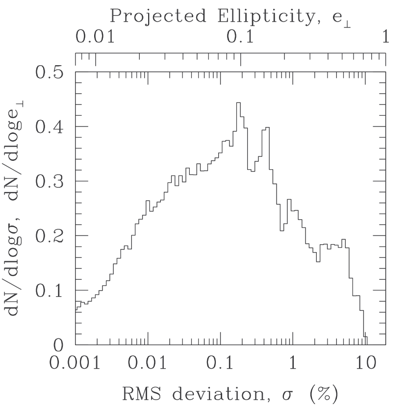
Figure 5.— The distribution of projected ellipticities of 551 chromospherically active giant stars in the Galactic bulge, as inferred from their colors, magnitudes, and rotation periods measured by OGLE II (Olech, 1996). The top axis labels show the inferred ellipticity, and the bottom axis labels shows the RMS light curve deviations that would occur (relative to a circular source) if the stars were to cross randomly oriented lensing caustics.

The three-dimensional ellipticity of a source is not observable in caustic-crossing events, rather only the ellipticity projected on the plane of the sky, $e_{\perp}=e(1-\cos^{2}{i})$. Here $i$ is the angle between the line-of-sight and the rotation axis of the star. For a ensemble of stars, this angle will be distributed uniformly in $\cos{i}$. The probability distribution of $e_{\perp}/e$ is thus, $P(e_{\perp}/e)=\frac{1}{2}[1-(e_{\perp}/e)]^{-1/2}$.

We note that there is a selection effect that introduces a bias in our determination of the distribution of projected ellipticities, which we make no attempt to correct. Nearly pole-on stars will have smaller variability amplitudes, and therefore will be preferentially missed by the OGLE survey. Therefore, our assumption that the distribution of $\cos{i}$ is uniform is not actually correct for this sample. We expect this bias to be relatively small, because systems have to be very close to pole-on to be missed (due to the excellent quality of the OGLE photometry), and because this bias will largely be washed out by the intrinsic scatter in the amplitudes of the photometric modulation due to, e.g. variable numbers and distributions of spots.

Figure 5 shows the resulting distribution of projected ellipticities for the 551 stars from the Olech (1996) catalog. The median ellipticity is $e=0.07$, with $\sim 20\%$ of stars have $e>0.2$. We relate the projected ellipticity to the RMS light curve deviation $\sigma$ by integrating equation (12) over $\phi$, which yields $\sigma\simeq 0.2e_{\perp}^{2}$. The median value is $\sigma\sim 0.1\%$, with $\gtrsim 15\%$ of stars expected to produce RMS deviations $\gtrsim 1\%$.

Current microlensing follow-up efforts can regularly achieve single-exposure precisions of $1\%$ on bright giant stars. Therefore, if the majority of giant stars in the bulge have rotation periods that are similar to those in the Olech (1996) sample, then $10-20\%$ of all caustic-crossing events should show deviations due to the stellar oblateness. Whether or not chromospherically quiescent stars should have similar rotation periods to active stars is not clear. Our analysis demonstrates that this question could be answered with a sample of $\sim 30$ precise, well-covered caustic-crossing events.

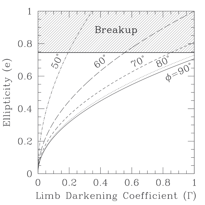
Figure 6.— The lines show the relation $e=[-0.5\Gamma\sec{2\phi}]^{1/2}$, the ellipticity $e$ required for a uniform, elliptical source to approximately reproduce the light curve of a limb-darkened circular source, as a function of the limb-darkening parameter $\Gamma$, for position angles of the elliptical source relative to the caustic normal of $\phi=0,10^{\circ},20^{\circ},30^{\circ}$, and $40^{\circ}$. Sources with $\phi=45^{\circ}$ produce no deviation due to ellipticity, and sources with $\phi<45^{\circ}$ produce deviations that are incompatible with limb-darkening. Values of $e\geq 0.745$ are not allowed for rotating stars, as they would be rotating faster than breakup speed.

One potential complication to the measurement of oblateness is limb-darkening. For a circular, limb-darkened source with radial surface brightness profile of the form

$$I(r)=1-\Gamma\left\{1-\frac{3}{2}\left[1-\left(\frac{r}{\rho}\right)^{2}\right]^{1/2}\right\},$$ (14)

the magnification of a limb-darkened source is (Albrow et al., 1999),

$$A(\eta;\Gamma)=A(\eta,0)+\left(\frac{u_{r}}{\rho}\right)^{1/2}\Gamma[G_{1/2}(\eta)-G_{0}(\eta)].$$ (15)

The form for the surface-brightness profile given in equation (14) was introduced in (Albrow et al., 1999). It is has the same behavior as the usual linear limb-darkening parameterization, but has the advantage that there is no net flux associated with the limb-darkening. The normalized limb-darkening function $G_{1/2}(\eta)-G_{0}(\eta)$ is shown in Figure 2.

It is clear that the form of the deviation due to the limb-darkening is qualitatively similar to the deviation due to oblateness for $\phi>45^{\circ}$, such that a limb-darkening circular source with $\Gamma\sim-2e^{2}\cos(2\phi)$ approximately reproduces the light curve of a uniform elliptical source with parameters $e,\phi$. The factor of two is the ratio of the RMS deviations of $E(\eta)$ and $G_{1/2}(\eta)-G_{0}(\eta)$ for $-1\leq\eta\leq 1$. The value of $e$ required to produce a given limb-darkening $\Gamma$ is plotted in Figure 6, for several values of $\phi$. Figure 2 shows an example, for a limb-darkened circular source with $\Gamma=0.5$, and a uniform, elliptical source with $e=0.5$ and $\phi=90^{\circ}$. Other examples are shown in Figure 3. The degeneracy is only approximate, however the two curves agree well except near the beginning and end of the caustic crossing. Note that, in general, the time when the source exits the caustic (near $\eta\sim-1$) will be different for circular and elliptical sources of equal area.

Of course, stars will, in general, be both oblate and limb-darkened. We find numerically that for small ellipticities, the light curve of an elliptical, limb-darkened source is well-approximated by the superposition of the effects of limb-darkening and ellipticity. In the optical to near-infrared, limb-darkening parameters for typical microlensing stars are in the range $\Gamma=0.3-0.7$ (Fields et al., 2003), and therefore limb-darkening effect will typically dominate over the effect of ellipticity. However, given the extraordinary precision of recent limb-darkening measurements (Fields et al., 2003; Abe et al., 2003), it is not clear that the effect of oblateness can be ignored. In particular, the inconsistency claimed by Fields et al. (2003) between derived limb-darkening parameters of the K3 III source of microlensing event EROS BLG-2000-5 and stellar atmospheric model model predictions may be partly reconciled by allowing for stellar oblateness. Fortunately, in this case a spectrum is available from which the $v\sin{i}$ of the star can be constrained. However, in the future, modelers should be aware of this possible contamination to limb-darkening measurements.

How can oblateness be distinguished from limb-darkening? First, since the effects are not completely degenerate, this may be possible to distinguish between them simply from high-precision, single-color measurements. Second, the oblateness signal is expected to be achromatic, whereas limb-darkening depends strong on wavelength. Finally, one can use multiple caustic crossings to attempt to distinguish between limb-darkening and oblateness: a second caustic crossing can be anticipated, and in general, it would occur at a different angle $\phi$ from the first.

3.2. Oblateness of Extrasolar Planets

Graff & Gaudi (2000) and Lewis & Ibata (2000) demonstrated that close-in, giant planetary companions to the source stars of binary microlensing events can be detected if the planet crosses a fold caustic, which magnifies the reflected starlight to detectable levels. Subsequently, Ashton & Lewis (2001) and Gaudi, Chang, & Han (2003) explored the detectability of structures associated with planets using this method, such as the planetary phase, atmospheric features, satellites, and rings. These authors found that, while the planet itself may be detectable, as well as variations due to the planet phase and associated rings, all other features are likely to be undetectable with foreseeable telescopes.

Can the oblateness of giant planets be detected via this method? Gaudi, Chang, & Han (2003) calculated the expected signal-to-noise ratio $Q_{p}$ of the primary planet signal for a typical event. They found $Q_{p}\sim 150(D/100{\rm m})^{2}(a/0.05~{}{\rm AU})^{-2}$, where $D$ is the telescope aperture and $a$ is the semi-major axis of the planet orbit. From equation (12), the signal-to-noise ratio $Q_{e}$ of the deviation due to ellipticity, averaged over all $\phi$, can be related to $Q_{p}$ by

$$Q_{e}\sim 0.2e^{2}Q_{p}\sim 30e^{2}\left(\frac{D}{100{\rm m}}\right)^{2}\left(\frac{a}{0.05~{}{\rm AU}}\right)^{-2}.$$ (16)

Thus we can expect signal-to-noise ratios of less than unity for the deviation due to ellipticity, unless the ellipticity is quite large, $e\gtrsim 0.2$. On the other hand, close-in giant planets with $a\lesssim 0.2~{}{\rm AU}$ are expected to be tidally locked to their parent star, and therefore their oblateness due to rotation are expected to be quite small, $f\lesssim 0.3\%$ or $e\lesssim 10\%$ (Seager & Hui, 2002). Planets whose rotation periods have not been synchronized with their orbital periods may have large oblateness. For example Jupiter has an oblateness of $f\sim 0.065$, which corresponds to an eccentricity of $e\sim 0.34$. Unfortunately, the amount of reflected light, and therefore the signal-to-noise ratio, falls off as $a^{-2}$, decreasing the signal-to-noise ratio of the planet signal by a factor of $\gtrsim 16$ for tidally-unaffected planets with $a\gtrsim 0.2$, and therefore rendering the distant planets too faint for the oblateness signal to be detectable, even if they are rapidly rotating.

3.3. Accretion Disks

Numerous authors have considered the idea of using microlensing of multiply-imaged quasars to resolve the surface brightness distribution of the central accretion disk. Studies range from theoretical examinations of the feasibility and details of the method itself (e.g., Grieger, Kayser, & Refsdal 1988; Grieger, Kayser, & Schramm 1991; Agol & Krolik 1999), to detailed fitting of light curves of the lens Q2237+0305 (e.g., Yonehara 2001; Shalyapin et al. 2002; Goicoechea et al. 2003; Kochanek 2003). The majority of these studies considered source models of face-on accretion disks. This assumption is generally not appropriate for standard geometrically-thin accretion disks: disks are more likely to be seen edge-on than face-on. Here we briefly consider the signature of inclined accretion disks on fold caustic-crossing light curves, and in the process uncover a degeneracy between the inclination and position angle for disks with self-similar intensity profiles. For simplicity, we consider only linear fold caustics. However, we note that this assumption may be inappropriate for typical quasar microlensing scenarios, which have relatively large sources, and optical depths to microlensing near unity (Wyithe, Webster, & Turner, 2000; Kochanek, 2003). Lensing of an inclined disk by a point mass was considered by (Heyrovsky & Loeb, 1997).

Figure 7.— (a) Normalized surface brightness profiles $rI_{\nu}(r)$ as a function of radius $r/R_{\rm S}$ in units of the Schwarzschild radius, for a standard thin accretion disk with inner radius $3R_{\rm S}$. Profiles are shown for three different values of the radius $R_{\nu}$ where the temperature of the accretion disk is equal to $h\nu/k$: $R_{\nu}=10R_{\rm S}$ (solid), $R_{\nu}\simeq 25R_{\rm S}$ (dashed), and $R_{\nu}\simeq 4R_{\rm S}$ (dotted). (b) Magnification as a function of time in units of $\Delta t=R_{\nu}/v_{e}$, where $v_{e}$ is the effective source transverse velocity. The curves correspond to the surface brightness profiles in panel (a). We have assumed that the disk has inclination $i=30^{\circ}$, position angle relative to the caustic normal of $\phi=15^{\circ}$, an Einstein ring radius of $\theta_{\rm E}D_{\rm os}=100R_{\rm S}$, and that the magnification outside the caustic is $A_{0}=3$.

We consider a standard, optically-thick, geometrically-thin accretion disk (Shakura & Sunyaev, 1973). The disk radiates locally as a blackbody with temperature,

$$T(r)=T_{\nu}\left(\frac{r}{R_{\nu}}\right)^{-3/4}\left[1-\left(\frac{r}{3R_{\rm S}}\right)^{-1/2}\right]^{1/4},$$ (17)

where $r$ refers to the radial distance of a (face-on) disk from the center, and we have assumed an inner disk edge of $3R_{\rm S}$. Here $R_{\nu}$ is the radius at which the local temperature of the disk matches the wavelength of observations, i.e. where $T(r)=T_{\nu}=h\nu/k$. Under the assumption of a standard thin-disk model, $R_{\nu}$ can be related to the mass of the black hole and the mass accretion rate. The surface brightness profile is then,

$$I_{\nu}(r)\propto\left({\rm e}^{T_{\nu}/T(r)}-1\right)^{-1}.$$ (18)

Note that we have ignored all relativistic and Doppler effects. Figure 7 shows the normalized surface brightness profile for the assumption of $R_{\nu}=10R_{\rm S}$, which roughly corresponds to the value found by Kochanek (2003) from an analysis of OGLE light curves of Q2237+0305 in the $V$-band, corresponding to rest-frame $2000$Å. We also show surface brightness profiles for $R_{\nu}=2^{4/3}10R_{\rm S}$ and $R_{\nu}=2^{-4/3}10R_{\rm S}$, i.e. for half and twice the frequency of observations, respectively.

We calculate the light curves by first determining the image areas of a finite number of concentric elliptical annuli using the exact form for the magnification (Eq. 3). The ellipticity of a disk with inclination angle $i$ (where $i=0$ is face on) is $e=(1-\cos^{2}{i})^{1/2}$. We weight each annulus by the local surface brightness, which is simply given by equation (18), with $r$ replaced by the semi-major axis of the elliptical annulus. The magnification is then the sum over all annuli of the surface-brightness weighted image area, divided by the surface-brightness weighted area of the source. We integrate out to $r=10R_{\nu}$, beyond which we find that the contribution to the magnification is negligible. Figure 7 shows light curves for a standard thin accretion disk with inclination $i=30^{\circ}$ and position angle relative to the caustic normal of $\phi=15^{\circ}$. The units of time are $\Delta t=R_{\nu}/v_{e}$, where $v_{e}$ is the effective source transverse velocity. In addition, we have adopted parameters appropriate to Q2237+0305, namely an Einstein ring radius of $\theta_{\rm E}D_{\rm os}=100R_{\rm S}$, and a total magnification of images unrelated to the caustic of $A_{0}=3$ (see, e.g. Kochanek 2003). For this system, and $V$-band observations, $\Delta t\sim 60~{}{\rm days}$.

Figure 8.— Contours show the $1\sigma$ confidence limits on the inclination $i$ and position angle $\phi$, for simulated observations of a thin accretion disk crossing a linear fold caustic, with input parameters $i=20^{\circ}$ and $\phi=15^{\circ}$, shown as the cross. We have assumed 100 measurements from $-10\leq\Delta t\leq 10$, each with $2\%$ error, and a background magnification of $A_{0}=3$. The lines types correspond to light curves in Figure 7, and are for $R_{\nu}=10R_{\rm S}$ (solid), $R_{\nu}\simeq 25R_{\rm S}$ (dashed), and $R\nu\simeq 4R_{\rm S}$ (dotted).

In §2 we demonstrated analytically that the light curves of uniform, equal-area elliptical sources with $e\ll 1$ are degenerate in $e$ and $\phi$ , such that one can only measure the combination $e^{2}\cos{2\phi}$. In fact, as could have been anticipated from Figure 4, we find numerically that the degeneracy between $e$ and $\phi$ exists for arbitrary ellipticities, again provided that the sources are normalized to have equal area. In turn, this implies that the degeneracy between $e$ and $\phi$ exists for any source with surface brightness profile that is elliptical and scale-free. The scale-free requirement arises from the fact that the ellipses must have equal-area, which implies different values for the semi-major axes. Therefore the introduction of a scale in the surface brightness profile will break the degeneracy. For accretion disks, the degeneracy translates into a degeneracy between $i,\phi$, and $R_{\nu}$. However, since the profile $I_{\nu}(r)$ of a standard thin disk (Eq. 18) is not scale-free, this degeneracy is not perfect. The severity of the degeneracy is set by the radius of the inner edge of the disk relative to $R_{\nu}$. If $R_{\rm S}/R_{\nu}\ll 1$, the surface brightness profile will essentially be scale-free, and the light curves will be degenerate. However, if $R_{\rm S}/R_{\nu}\sim 1$, the central hole in the surface brightness profile of the disk creates a feature in the light curve (see Figure 7). Larger inclinations will produce more pronounced features due to this central hole, thus allowing one to distinguish the light curve produced from different inclinations. We note that this degeneracy was likely present in the simulations of Agol & Krolik (1999), although it does not seem to have been explicitly recognized as such.

To crudely quantify the severity of this degeneracy, we have simulated observations of a caustic-crossing event. We adopted the parameters of the light curves shown in Figure 7, namely $i=30^{\circ}$, $\phi=15^{\circ}$, $\theta_{\rm E}D_{\rm os}=100R_{\rm S}$, and $A_{0}=3$. We assume 100 equally-spaced observations from $-10\leq\Delta t\leq 10$, each yielding photometry in a single band with a fractional flux error of $2\%$. For the parameters of Q2237+0305, this corresponds to a sampling interval of $\sim 12~{}{\rm days}$. This sampling interval and photometric error are comparable to that in the OGLE light curve of Q2237+0305 (Woźniak et al., 2000). Figure 8 shows the resulting $1\sigma$ confidence regions in the $i,\phi$ plane for the three different light curves. As expected, the degeneracy is most severe for $R_{\nu}=25R_{\rm S}$, where inclinations as large as $80^{\circ}$ are consistent with the simulated light curve at the $1\sigma$ level. This translates into a factor of $(\cos{30^{\circ}}/\cos{80^{\circ}})^{1/2}\sim 2$ uncertainty in $R_{\nu}$. Note that we have fixed all other free parameters at their input values; allowing these parameters to vary would worsen the degeneracy.

Since a measurement of $R_{\nu}$ can be used to constrain the mass of the black hole, it is important to reduce the uncertainty in $R_{\nu}$ if possible. This can be done by obtaining higher-precision observations, although we find that, for the same sampling rate, the precision of the individual measurements must be $\lesssim 0.2\%$ to reduce the uncertainty to below $20\%$. A more robust way of reducing this uncertainty is to observe at higher frequencies, where the ratio $R_{\rm S}/R_{\nu}$ is larger. For example, for $R_{\nu}=10R_{\rm S}$, the uncertainty in $R_{\nu}$ is only $\sim 10\%$. Higher frequencies are desirable for two additional reasons. First, since $R_{\nu}$ is smaller, the source is more compact, which results in a higher magnification as the source crosses the caustic, improving the signal-to-noise ratio. Second, Doppler and relativistic effects are larger for radii closer to the black hole. These effects impose asymmetries in the surface brightness of the disk, which further reduce degeneracies between the parameters, and may even enable a measurement of the black hole spin (Agol & Krolik, 1999).

It is also important to note that we have assumed observations of a single, linear caustic-crossing event. Observations of multiple caustic-crossings, or observations of crossings of more complicated caustic geometries (i.e. parabolic folds, cusps, etc.), would likely remove this degeneracy. However, the additional complexity of such geometries may give rise to other complications and new degeneracies; addressing these issues is beyond the scope of the present paper.

4. Summary

Fold caustics are germane to many applications of gravitational microlensing. Previous studies have primarily focused on sources with circular symmetry. Here we have considered microlensing of elliptical sources by fold caustics. We considered only linear fold caustics, which are generally applicable when the size of the source is much smaller than the Einstein ring radius of the system, and prove a useful and analytic approximation to the magnification structure near real fold caustics. The total magnification of the two images produced near such a caustic is proportional to the square-root of the perpendicular distance to the caustic, and thus diverges as a point source approaches the caustic. The chief utility of fold caustics is that this divergence can be used to achieve high spatial resolution and large magnification of faint or otherwise unresolved sources.

By convolving the magnification near a fold caustic with sources of arbitrary ellipticity, we computed the magnification of a source near a fold caustic of scale $u_{r}$ as a function of its ellipticity $e$, position angle $\phi$ of the major axis with respect to the caustic normal, area $\pi\rho^{2}$, and separation from the caustic $\eta\rho$. We demonstrated that, for $e\ll 1$, the deviation due to ellipticity is simply $(u_{r}/\rho)^{1/2}e^{2}\cos{2\phi}E(\eta)$, where $E(\eta)$ is simple one-parameter function that can be trivially evaluated numerically or expressed in terms of elliptic integrals. The next higher-order corrections to this expression are of order $e^{4}$, and thus it is accurate to $\lesssim 1\%$ for $e\lesssim 0.3$. From this expression, it is clear that the deviation due to ellipticity vanishes for $\phi=45^{\circ}$, and one can only measure the combination of parameters $e^{2}\cos{2\phi}$ from observations of a single fold caustic crossing. For $e\ll 1$, the root-mean-square light curve deviation due to ellipticity in the range $-1\leq\eta\leq 1.5$ is $0.3e^{2}\cos{2\phi}$. Surprisingly, we found that the deviation due to ellipticity vanishes at some value of $\phi\geq 45^{\circ}$, for all values of $e$, with $\phi>45^{\circ}$ for $e\gtrsim 0.3$ and increasing with increasing ellipticity.

We considered three applications of microlensing of elliptical sources near fold caustics. We first demonstrated that, if most of the microlensing source stars have rotation periods similar to chromospherically active, spotted stars in the bulge, then approximately $\sim 15\%$ should exhibit light curve deviations due to their oblateness (corresponding to ellipticities $e\gtrsim 0.2$) that are detectable with current observations. The deviation due to limb-darkening is qualitatively similar to that due to ellipticity, such that a uniform elliptical source with parameters $e,\phi$ can approximately reproduce the light curve of a circular, limb-darkened source with $\Gamma=-2e^{2}\cos{2\phi}$. This may complicate the interpretation of ultra-precise measurements of limb-darkening with microlensing. We then considered the feasibility of detecting the oblateness of close-in, giant, planetary companions to the source-stars of caustic-crossing microlensing events. We found that planets which are sufficiently close to provide a detectable reflected light signal are also generally tidally locked, and therefore rotating too slowly to produce a substantial deviation due to oblateness. If tidal locking can be prevented to preserve an ellipticity of $e\gtrsim 0.2$ even in the close-in planets, then the oblateness may be observable, especially for fortuitous geometries (with caustic crossing occurring along the direction perpendicular to the major or minor axis). Finally, we considered the resolution of the structure of a quasar accretion disks using microlensing by stars in the foreground lens of a multiply-imaged quasar. We showed that there exists a partial degeneracy between the disk inclination, scale length, and position angle for the orientation of the projected ellipse relative to the caustic. For passbands primarily arising from the outer portion of the disk, this degeneracy can lead to a factor of two uncertainty in the determination the disk scale length, which translates directly into an uncertainty in the black-hole mass, in the standard thin accretion disk model. Higher-frequency or higher-precision observations can reduce this uncertainty.

References

- Abe et al. (2003) Abe, F. et al. 2003, A&A Letters, in press (astro-ph/0310410)
- Agol & Krolik (1999) Agol, E. & Krolik, J. 1999, ApJ, 524, 49
- Albrow et al. (1999) Albrow, M. D. et al. 1999, ApJ, 522, 1011
- Albrow et al. (2000) Albrow, M. D. et al. 2000, ApJ, 534, 894
- Albrow et al. (2001) Albrow, M. D. et al. 2001, ApJ, 549, 759
- Alcock et al. (2000) Alcock, C. et al. 2000, ApJ, 541, 270
- Ashton & Lewis (2001) Ashton, C. E. & Lewis, G. F. 2001, MNRAS, 325, 305
- Dominik (2003) Dominik, M. 2003, MNRAS, submitted (astro-ph/0309581)
- Fields et al. (2003) Fields, D. L. et al. 2003, ApJ, 596, 1305
- Gaudi & Gould (1999) Gaudi, B. S. & Gould, A. 1999, ApJ, 513, 619
- Gaudi & Petters (2002) Gaudi, B. S. & Petters, A. O. 2002, ApJ, 574, 970
- Gaudi, Chang, & Han (2003) Gaudi, B. S., Chang, H., & Han, C. 2003, ApJ, 586, 527
- Goicoechea et al. (2003) Goicoechea, L. J., Alcalde, D., Mediavilla, E., & Muñoz, J. A. 2003, A&A, 397, 517
- Gould (2001) Gould, A. 2001, PASP, 113, 903
- Gould & Miralda-Escude (1997) Gould, A. & Miralda-Escude, J. 1997, ApJ, 483, L13
- Graff & Gaudi (2000) Graff, D. S. & Gaudi, B. S. 2000, ApJ, 538, L133
- Grieger, Kayser, & Refsdal (1988) Grieger, B., Kayser, R., & Refsdal, S. 1988, A&A, 194, 54
- Grieger, Kayser, & Schramm (1991) Grieger, B., Kayser, R., & Schramm, T. 1991, A&A, 252, 508
- Hendry et al. (1998) Hendry, M. A., Coleman, I. J., Gray, N., Newsam, A. M., & Simmons, J. F. L. 1998, New Astronomy Review, 42, 125
- Hendry, Bryce, & Valls-Gabaud (2002) Hendry, M. A., Bryce, H. M., & Valls-Gabaud, D. 2002, MNRAS, 335, 539
- Heyrovsky (2003) Heyrovsky, D. 2003, ApJ, 594, 464
- Heyrovsky & Sasselov (2000) Heyrovsky, D., & Sasselov, D. 2000, ApJ, 529, 69
- Heyrovsky & Loeb (1997) Heyrovsky, D., & Loeb, A. 1997, ApJ, 490, 38
- Kochanek (2003) Kochanek, C.S. 2003, ApJ, submitted (astro-ph/0307422)
- Lewis & Ibata (2000) Lewis, G. F. & Ibata, R. A. 2000, ApJ, 539, L63
- Jaroszyński & Mao (2001) Jaroszyński, M. & Mao, S. 2001, MNRAS, 325, 1546
- Olech (1996) Olech, A. 1996, Acta Astronomica, 46, 389
- Seager & Hui (2002) Seager, S. & Hui, L. 2002, ApJ, 574, 1004
- Petters, Levine, & Wambsganss (2001) Petters, A. O., Levine, H., & Wambsganss, J. 2001, Singularity Theory and Gravitational Lensing (Boston : Birkhäuser)
- Schneider, Ehlers & Falco (1992) Schneider, P., Ehlers, J., & Falco, E. E. 1992, Gravitational Lenses (Berlin: Springer)
- Shakura & Sunyaev (1973) Shakura, N. I. & Sunyaev, R. A. 1973, A&A, 24, 337
- Shalyapin et al. (2002) Shalyapin, V. N., Goicoechea, L. J., Alcalde, D., Mediavilla, E., Muñoz, J. A., & Gil-Merino, R. 2002, ApJ, 579, 127
- Udalski et al. (2000) Udalski, A., Zebrun, K., Szymanski, M., Kubiak, M., Pietrzynski, G., Soszynski, I., & Wozniak, P. 2000, Acta Astronomica, 50, 1
- Valls-Gabaud (1998) Valls-Gabaud, D. 1998, MNRAS, 294, 747
- van Belle (1999) van Belle, G. T. 1999, PASP, 111, 1515
- Woźniak et al. (2000) Woźniak, P. R., Udalski, A., Szymański, M., Kubiak, M., Pietrzyński, G., Soszyński, I., Żebruń, K. 2000, ApJ, 540, L65
- Wyithe, Webster, & Turner (2000) Wyithe, J. S. B., Webster, R. L., & Turner, E. L. 2000, MNRAS, 318, 1120
- Yonehara (2001) Yonehara, A. 2001, ApJ, 548, L127