The very high state accretion disc structure from the galactic black hole transient XTE J1550-564

Abstract

The 1998 outburst of the bright Galactic black hole binary system XTE J1550-564 was used to constrain the accretion disc structure in the strongly Comptonised very high state spectra. These data show that the disc emission is not easily compatible with the constant area $L\propto T^{4}$ behaviour seen during the thermal dominated high/soft state and weakly comptonised very high state. Even after correcting for the effects of the scattering geometry, the disc temperature is always much lower than expected for its derived luminosity in the very high state. The simplest interpretation is that this indicates that the optically thick disc is truncated in the strongly Comptonised very high state, so trivially giving the observed continuity of properties between the low/hard and very high states of Galactic black holes.

1 Introduction

Accreting black holes in our Galaxy show a large variety of X-ray properties, which can be classified into distinct spectral states (Tanaka & Lewin 1995; McClintock & Remillard 2003, hereafter MR03). In the high/soft state, typically seen at luminosities above $\sim 5-10$ per cent of Eddington, the energy spectrum is dominated by a soft thermal component of temperature 0.4– 1.5 keV. This is well described by the standard accretion model of emission from an optically thick and geometrically thin disc (Shakura & Sunyaev 1973, hereafter SS73). Where the source varies, the temperature and luminosity of this disc component change together in such a way as to indicate that the size of the emitting structure remains approximately constant i.e. $L\propto T^{4}$ (Ebisawa et al.  1991; 1994; Kubota, Makishima & Ebisawa 2001; Kubota & Makishima 2004; hereafter KM04; Gierlinski & Done 2004; hereafter GD04). Excitingly, this gives an observable diagnostic of the mass and spin of the black hole, assuming that this constant size scale is set by the innermost stable orbit around the black hole.

These results are actually very surprising in the context of the SS73 disc equations. The predicted disc structure is violently unstable at such luminosities, where radiation pressure dominates, yet these disc dominated spectra show very little short time-scale variability. Also, the disc spectrum should not be a simple sum of blackbody spectra at these high temperatures, as electron scattering dominates over true absorption. In the X-ray band, this difference in spectral shape can be roughly described as a standard disc spectrum, but of a higher temperature than the effective (blackbody) temperature (Shimura & Takahara 1995; Merloni et al. 2000). However, this colour temperature correction factor can change with luminosity, so is not predicted to produce a simple $L\propto T^{4}$ relation (GD04).

Real discs are then observed to be much simpler than the SS73 predictions, pointing to the inadequacies of the ad hoc $\alpha$ viscosity prescription and motivating further studies of the disc structure which results from the physical (magnetic dynamo) viscosity mechanism in radiative discs (e.g. Turner 2004). This observed simplicity is reserved only for the high/soft state data, where the disc spectrum is dominant. Accreting black holes can also show a rather different type of spectrum at high luminosities, the so-called very high state termed the steep power-law state by MR03), characterized by a very strong (roughly) power-law component (Miyamoto et al. 1991). This is normally steep, with photon spectral index $\Gamma>2.2$, rather different to the standard low/hard state spectra seen usually at much lower luminosities (e.g. the reviews by Tanaka & Lewin 1995; MR03). In this very high state, the constant area inferred from the relation between observed temperature and disc luminosity breaks down (Ebisawa et al. 1994; Kubota et al. 2001; KM04; MR03).

To some extent this breakdown is expected. The strong high energy emission shows that a large fraction of the accretion energy is dissipated in some non-disc structure (corona/jet?), so the disc structure should be different to that seen when the emission is dominated by the thermal disc spectrum (e.g. Svensson & Zdziarski 1994). Also, the intense X-rays may illuminate the disc, again changing its structure (e.g. Nayakshin, Kazanas & Kallman 2000). However, Kubota et al (2001) showed that for very high state spectra where the high energy emission was less than $\sim 50$ per cent of the total flux (which they termed the anomalous spectra), then the constancy of disc area could be (approximately) recovered by careful modelling of the spectrum, and by correcting the observed disc luminosity to include the Compton scattered photons (KM04).

Here we investigate the extremely Comptonised very high state spectra from the 1998 outburst of XTE J1550-564, where the steep power law tail dominates the total emission. This source has a superluminal jet (Hannikainen et al. 2001) and is a confirmed black hole with mass of 8.4–11.2 $M_{\odot}$, at a distance of 5 kpc and binary inclination angle of $70^{\circ}$ (Orosz et al.  2002).

We show that these extremely Comptonised very high spectra are qualitatively and quantitatively different to the spectra with a weaker Comptonised tail. They are not easily compatible with a simple Comptonising corona above an untruncated disc, though such a geometry may be possible with a complex corona, with strong radial gradients in the optical depth. However, the simplest solution is that the disc in these Compton dominated spectra is truncated at larger radii than the minimum stable orbit around the black hole.

2 Spectral evolution of XTE J$1550-564$ in the 1998 outburst

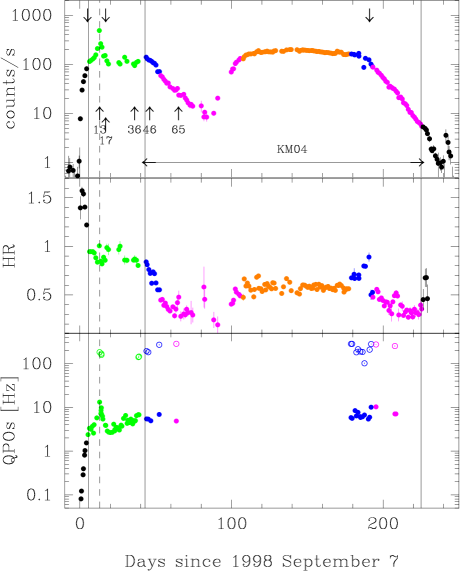
Figure 1: The RXTE ASM light curves of XTE J$1550-564$. The top panel shows the 1.5–12 keV ASM count rate, while the middle panel shows the ASM hardness ratio (5–12 keV/3–5 keV). The bottom panel shows the high (open circles) and low (filled circles) frequency QPOs, taken from Remillard et al.  (2002). Harmonics of the low frequency QPOs, reported by Remillard et al.  (2002), are not shown here. The times of the simultaneous ASCA/RXTE observations are indicated with down-arrows in the top panel, while up-arrows indicate the times of the spectra shown in Fig. 2. Vertical solid lines show days 5, 43, and 225 since the beginning of the outburst, and the vertical dashed line indicates the position of the outburst peak. Data points with blue, magenta, and orange correspond to the anomalous regime (or weak very high state in text), standard regime, and apparently standard regime defined by KM04, respectively. Green data points correspond to the strong very high state which is introduced in this paper.

The transient black hole binary XTE J$1550-564$ was discovered on 1998 September 7 by RXTE ASM (Smith 1998) and CGRO BATSE (Wilson et al. 1998). This source showed four subsequent outbursts since its discovery, but the first outburst was the brightest and best covered by RXTE pointing observations. The data were analyzed by many authors including Sobczak et al.  (1999; 2000ab), Wilson & Done (2001), Homan et al. (2001), and KM04.

Figure 1 shows the 1.5–12 keV light curve and hardness ratios of the first outburst, obtained with RXTE ASM, together with the frequency of the main QPO (where seen) from Remillard et al. (2002). Clearly the source hardness changes dramatically during the outburst, as does the QPO frequency. These are generally correlated, so that spectral states can be defined either from spectral or power spectral characteristics (van der Klis 2000; MR03).

Here we briefly summerise the main features of the source behaviour. The marked softening of the spectrum in the first 5-10 days after the source was detected is associated with a state transition from the low/hard state (first five days) into the very high state (Wilson & Done 2000; Cui et al. 1999; Sobczak et al. 1999). For about a month (between days 5–52: Fig. 1), the source showed strong QPOs and a strong hard spectral component (e.g., Sobczak et al. 2000a), so can be classified as in the very high state during the whole of this time. The QPO frequency changes quite dramatically during the first $\sim$ 40 days of the outburst, but then stabilizes from day 40-52. The type of QPO also changes at day 40 (from C/C’ to B: see Remillard et al.  2002).

After the day 52, the luminosity and hardness both decreased as the source made a transition to the classic high/soft disc dominated (termed thermal dominated: MR03) state. Generally the QPO is not seen, but when it is detected, it is of different type (A, very weak: Remillard et al. 2002) to that seen previously. Most of the time until the end of this first outburst, the source stayed in this disc dominated high/soft state as the luminosity changed, giving progressively higher/lower disc temperatures and so higher/lower hardness ratios. There is just one section (days 180-200) where the hard power law flux again increased relative to the disc emission to a level comparable to that seen towards the end of the first very high state (days 40-52) and where the QPOs (mainly type B) reappear. Hence Homan et al. (2001) identify these data as very high state.

The luminosity and temperature of the disc component from day 40 onwards is always consistent with optically thick material extending down to the last stable orbit around the black hole (KM04, see also Figs 4b-d). In this paper, we concentrate our discussion on the very high state spectra where the coronal luminosity is $>$ 50% of the total i.e. days 5–40 of the outburst. We will show that these data are most easily described if the inner disc does NOT extend down to the last stable orbit, as also indicated by the QPO frequency. Hereafter, we distinguish these data from the other very high states in which the power law component is weaker (days 40–52, 180–200), and call it the ”strong very high state”. In Table 1, we summarize the correspondence of the spectral states we used in this paper to the state defined in other literatures.

Table 1: Correspondence of the definition of the state name to those in other papers.

This paper	KM04	classic classification	MR03	QPO type †	corresponding obs.	Remarks ‡
low/hard	—	low/hard (low)	hard	C or C’	0–5	thermal IC
strong very high	—	very high (high)	SPL	C or C’	5–40	thermal IC
weak very high	anomalous	very high (high)	SPL	B∗	40–52, 180–200	thermal IC
standard high/soft	standard	high/soft (high)	TD	A or none	52–100, 200–220	dominant disc + PL
(apparently standard)§	apparently standard	high/soft (high)	TD	none	100–180	dominant disc + weak PL
† By referring to Remillard et al. 2002
‡ Characteristics of X-ray spectrum
∗ Majority of QPOs are found in type B, while type A and B QPOs are reported on day 192 and day 187, respectively.
§ Not described in the text.

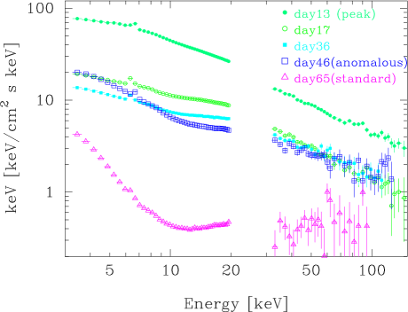
Figure 2: Typical PCA and HEXTE spectra of XTE J$1550-564$ taken from times as indicated in Fig. 1. The data is unfolded with the best fit model fit to the PCA+HEXTE data (see §4.2).

3 Data reduction

We used all the data from the first outburst except for the first 5 days where the source is in the low/hard state. Good PCA and HEXTE data were selected and processed, following the same procedures as in KM04 and WD01, respectively.

For the PCA data reduction we used top and mid layer from all available units, using standard exclusion criteria (target elevation less than $10^{\circ}$ above the Earth’s limb, pointing direction was more than $1^{\prime}\!.2$ from the target, data acquired within 30 minutes after the spacecraft passage through South Atlantic Anomaly). The standard dead time correction procedure was applied to the data. The PCA background was estimated for each observation, using the software package pcabackest (version 2.1e), supplied by the RXTE Guest Observer’s Facility at NASA/GSFC. The PCA response matrix was made for each observation by utilizing the latest version (8.0) of the software package pcarsp. In order to take into account the calibration uncertainties, 0.5% systematic errors are added to each bin of the PCA spectra. A more conservative 1% systematic error does not qualitatively change the results, but gives very small values of $\chi^{2}/{\rm dof}$. The 3–20 keV data are used in this paper, since there is sometimes residual structure in the 20–35 keV range associated with the Xe-K edge at $\sim$30 keV.

The HEXTE consists of two independent clusters (Cluster 0 and 1) of four NaI(Tl)/CsI(Na) phoswich scintillation counters (Rothschild et al. 1998). The HEXTE data were selected in the same way as that of the PCA. Since one detector on Cluster 1 of the HEXTE has lost its spectral capability, we use only Standard mode data from Cluster 0. The HEXTE background was subtracted by sequential rocking of the two clusters on and off of the source position. We used the software package called hxtback for splitting the data and the background. The HEXTE data below $30~{}$ keV were not used in the spectral fit because of response uncertainties associated with the Xe-K edge. Systematic errors of 0.5% are also added to each spectral bin of the HEXTE, though these are much smaller than statistical errors of the HEXTE data in the range of 30–200 keV so make no difference to the spectral fits. Figure 2 shows the range of spectral shapes seen by the PCA and HEXTE data over the course of the outburst, taken from days of 13, 17, 36, 46, and 65 as denoted by the up-arrows in Fig. 1.

ASCA observations of this source were performed three times, on 1998 September 12, 24, and 1999 March 17, as indicated with down arrows in Fig. 1. There are simultaneous RXTE observations corresponding to each ASCA observation. The first simultaneous observation was just on the boundary of the low and very high state, while the third one was in the weak very high state (days 180-200). In this paper we are most interested in the strong very high state, so we choose to use only the second ASCA observation. The ASCA GIS events were extracted from a circular region of $6^{\prime}$ radius centered on the image peak, after selecting good time intervals in a standard procedure. A net exposure of 2.4 ks was obtained for this simultaneous pointing. Dead time fractions are determined from count rate monitor data (Makishima et al. 1996) as 85.6% for GIS2 and 87.3% for GIS3. Systematic errors of 1% are added to each spectral bin. We only use the GIS data since the SIS is strongly affected by pileup.

The well known difference in calibration between the GIS and the PCA has been fixed in the PCA response matrices in HEASOFT 5.2. Thus the data are fitted simultaneously in this paper.

Table 2: Best fit parameters of XTE J$1550-564$

day	$T_{\rm in}$	$\Gamma$	$T_{\rm e}$	$L_{\rm disk}$	$L_{\rm thc}$	$L_{\rm pow}$	smedge	line	$\chi^{2}/{\rm dof}$
	keV	$\Gamma_{\rm thc}$	keV	$(N_{\rm disk})$	$(N_{\rm thc})^{e}$
MCD + power-law (PCA)
17	$0.38^{+0.01}_{-0.02}$	$2.46\pm 0.01$	—	1.98	—	3.24	$E=8.0^{+0.3}_{-0.2}$ keV	$E=6.44\pm 0.08$ keV	24.0/36
							$\tau_{\rm max}=0.17^{+0.05}_{-0.03}$	EW=$67\pm 12$ eV
							width$=1.3^{+0.6}_{-0.5}$ keV
36	$0.90^{+0.08}_{-0.12}$	$2.33\pm 0.03$	—	0.56	—	1.97	$E=8.1\pm 0.4$ keV	$E=6.48^{+0.12}_{-0.05}$ keV	24.0/36
							$\tau_{\rm max}=0.5^{+0.5}_{-0.3}$	EW=$64^{+15}_{-19}$ eV
							width$=4^{+6}_{-2}$ keV
46	$1.05\pm 0.02$	$2.42\pm 0.03$	—	1.70	—	1.76	$E=8.6^{+0.3}_{-0.2}$ keV	$E=6.7^{+0.2}_{-0.1}$ keV	17.0/36
							$\tau_{\rm max}>2.0_{-1.3}$	EW=$45\pm 12$ eV
							width$=18^{+3}_{-12}$ keV
65	$0.72\pm 0.01$	$2.07\pm 0.04$	—	1.05	—	0.12	$E=8.6\pm 0.2$ keV	$E=6.5\pm 0.2$ keV	37.2/36
							$\tau_{\rm max}>2.0_{-0.5}$	EW=$68\pm 16$ eV
							width$=8^{+1}_{-2}$ keV
MCD + power-law + thcomp (PCA & HEXTE)
17	$0.65^{+0.08}_{-0.04}$	$2.32\pm 0.03$	$13\pm 2$	1.21	2.50	0.69	$E=7.9^{+0.4}_{-0.3}$ keV	$E=6.40\pm 0.08$ keV	35.9/72
				(29.9)	(42.9)		$\tau_{\rm max}=0.35\pm 0.13$	EW=$77^{+17}_{-9}$ eV
							width$=3\pm 2$ keV
36	$0.78^{+0.05}_{-0.06}$	$2.25\pm 0.04$	$22^{+30}_{-7}$	1.01	1.51	0.51	$E=7.9^{+0.4}_{-0.3}$ keV	$E=6.4\pm 0.1$ keV	49.4/72
				(22.2)	(20.2)		$\tau_{\rm max}=1.2^{>+0.8}_{-0.7}$	EW=$65^{+18}_{-13}$ eV
							width$=10^{+8}_{-6}$ keV
46	$0.98\pm 0.02$	$2.40\pm 0.08$	$19^{>+181}_{-8}$	2.13	1.08	0.72	$E=8.6^{+0.2}_{-0.1}$ keV	$E=6.7^{+0.2}_{-0.1}$ keV	50.8/72
				(38.2)	(13.8)		$\tau_{\rm max}>2.0_{-1.0}$	EW=$54\pm 12$ eV
							width$=15^{+2}_{-7}$ keV
Errors represent 90% confidence level for one free parameter i.e. $\Delta\chi^{2}=2.7$.
Normalization factors with the PCA data are used to calculate luminosities.

4 Analyses of the multiple RXTE data

4.1 Simple fits to the PCA data

In order to briefly characterize the spectral behavior throughout the outburst, we performed spectral fitting to the 3–20 keV PCA data with the canonical multicolour disc model (hereafter MCD model, diskbb in XSPEC; Mitsuda et al. 1984) plus a power-law model. The power-law component is modified by an absorption edge around 7–9 keV described by a smeared edge model (smedge in XSPEC; Ebisawa et al.  1994), and a narrow Gaussian is also added for the Fe-K line by constraining its central energy in the range 6.2–6.9 keV. The data of days 80–165 cannot constrain the power-law photon index so the index was fixed at 2.0, representing the mean HEXTE slope (Sobczak et al. 2000b; KM04). We fix the hydrogen column at $N_{\rm H}=7\times 10^{21}~{}{\rm cm^{-2}}$ as indicated by the ASCA data (see table 3), but otherwise the analysis is the same as in KM04.

Except for the data at the peak (day 13), this model fits the data adequately, and Table 2 gives the best fit parameters for the spectra shown in Fig. 2. Figure 3 shows the evolution of the spectral parameters as a function of time (as in Fig. 2 of KM04 but including the strong very high state data of the first 5–40 days as well). Panel (a) shows the bolometric luminosity of the disc, $L_{\rm disk}$, 1–100 keV power law luminosity, $L_{\rm pow}$ and total $L_{\rm tot}\equiv L_{\rm disk}+L_{\rm pow}$. Here, $L_{\rm disk}$ is calculated by referring to two parameters of the MCD model, inner disc temperature $T_{\rm in}$ (panel b) and an apparent inner disc radius $r_{\rm in}$ (panel c), as $L_{\rm disk}=4\pi r_{\rm in}^{2}\sigma T_{\rm in}^{4}$.

Figure 4a plots the derived disc luminosity against inner disc temperature for these fits. Clearly, $L_{\rm disk}\propto T_{\rm in}^{4}$ in the standard high/soft state (magenta filled circles), indicating a constant area emitting region. Only the very lowest luminosity points deviate from this line, but the errors on these are fairly large as the low temperature disc is rather poorly covered by the PCA bandpass. When we fit these data points with a power-law, we obtain an index of $3.9^{+0.1}_{-0.2}$ with a normalization at $T_{\rm in}=1$ keV of $L_{\rm disk}=3.55\pm 0.08~{}{\rm erg~{}s^{-1}}$. It is very tempting to identify the source of this markedly constant behaviour with the constant area defined by a disc extending down to the innermost stable orbit. When the apparent inner disc radius of $r_{\rm in}=53$ km derived from the fits is corrected for the stress–free inner boundary condition (Kubota et al. 1998) and colour temperature correction of 1.7 then this gives an estimate for the true inner disc radius of $R_{\rm in}=63$ km with a typical error of 10 %. This value is slightly smaller than 75–100 km, which is the innermost stable orbit for a non-spinning black hole of 8.4–11.2 $M_{\odot}$. Therefore, XTE J$1550-564$ is consistent with a moderately rotating black hole, while uncertainties of the source distance and determination of $\kappa$ can cancel this difference.

The behaviour of the disc component in the rest of the data is rather different. Fig. 4a shows that the strong very high state spectra (green open squares, days 5–30) have a much lower temperature disc than expected for the disc luminosity. Conversely the disc in the weak very high states has the disc at somewhat higher temperature than expected from its luminosity. In other words, the disc inner radius of the strong very high state appears at much larger values than that disc dominated regime, while that of the weak very high state is apparently found at smaller values. Inspection of Fig. 3(b)–(c) shows that this change in behaviour happens around day 30.

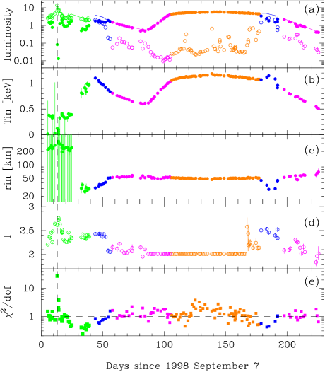
Figure 3: Evolution of the spectral parameters of XTE J$1550-564$ based on the PCA data fitted by a simple MCD plus power-law model (see § 4.1). (a)Time histories of $L_{\rm disk}$ (filled circles), $L_{\rm pow}$ (solid circles), and $L_{\rm tot}$ (solid line), all in units of $10^{38}\cdot{D_{5}}^{2}~{}{\rm erg~{}s^{-1}}$ and assuming $i=70^{\circ}$ for the disc emission. (b)–(e) Those of $T_{\rm in}$, $r_{\rm in}$, $\Gamma$, and $\chi^{2}/{\rm dof}$, respectively.

(a)MCD+power-law

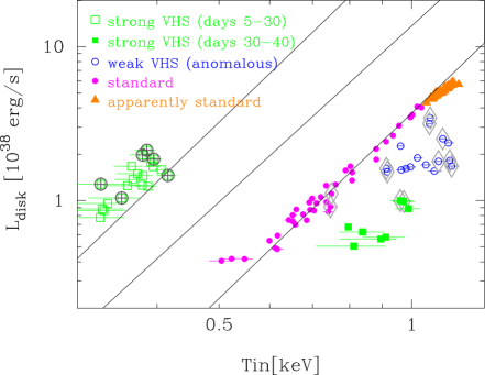
(b)MCD+thcomp+power-law

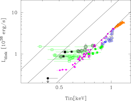
(c)MCD+thcomp+power-law

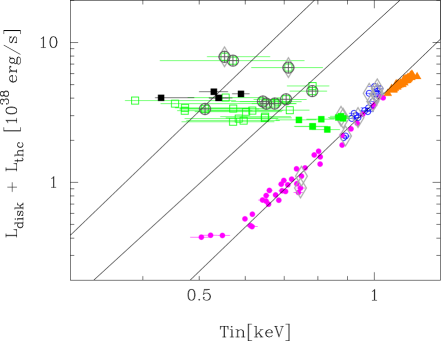
(d)MCD+thcomp+power-law

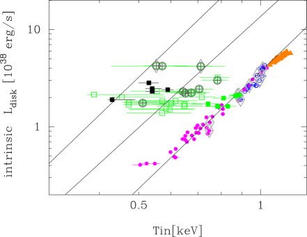
Figure 4: The disc luminosity plotted against the observed inner disc temperature, $T_{\rm in}$. (a) $L_{\rm disk}$ is taken from the MCD plus power-law model fits to the PCA data (§ 4.1). (b) $L_{\rm disk}$ is taken from the three-component model fits to the PCA+HEXTE data, including the thcomp model to describe the thermal Comptonisation (§ 4.2). (c) $L_{\rm disk}+L_{\rm thc}$ from the three-component model (§ 4.2). (d)) $L_{\rm disk}^{\rm int}$ estimated by conservation of photon number (§ 5). In all panels the solid lines show lines of constant apparent inner disc radius of 59, 100 and 200 km, with colours indicating different spectral states (see Fig 1. and table 1). Additionally, points highlighted by a large circle with a cross are those where there is also strong radio emission from the jet, while diamonds show the ones where the high frequency QPO is detected. Panels (b)-(d) also include the data from the five different fits to the ASCA-PCA-HEXTE spectrum (Table 3) as black squares. In panel (a), some data points around the peak are not included, and in panels (b)–(d), the data point at the peak is not included.

4.2 Fitting with the picture of the strong disc Comptonisation

The key characteristic of all the non high/soft state data is that the Comptonised tail is much more important in the spectrum (see Fig. 2), so details of how it is modeled become important. A power law approximation for the Comptonised spectrum is inadequate, as real Compton spectra show a low energy turnover close to the seed photon energy (KM04; Done, Zycki & Smith 2002). We replace the power law with a proper thermal Comptonisation model (thcomp in XSPEC: Zdziarski, Johnson & Magdziarz 1996) which is parameterized by asymptotic power law index, $\Gamma_{\rm thc}$, and electron temperature, $T_{\rm e}$. We assume that the seed photons are from the observed MCD component, so $T_{\rm e}$ is the only additional free parameter compared to the previous power law fits.

We use the PCA and HEXTE data in order to better constrain $T_{\rm e}$, but this broad bandpass shows that the spectra are rather more complex than a single thermal comptonisation component (and its reflected emission). While the data below 20 keV can be dominated by the disc and a cool thermal Compton component, the higher energy data show a quasi-power law tail (Gierlinski et al. 1999; Zdziarski et al. 2001; WD01; Kubota et al. 2001; Gierlinski & Done 2003; KM04). We follow KM04 and model this additional component as a power law with photon index $\Gamma$ fixed at 2.0 which is the average index of the high energy emission in the standard high/soft state (e.g. fits to HEXTE data: Sobczak et al. 2000b), and fit all the PCA+HEXTE data with this three component continuum model; MCD plus thermal comptonisation (thcomp) plus power law, with the gaussian line and smeared edge to mimic reflection. All the model parameters are constrained to be the same between the PCA and the HEXTE data except for a normalization factor.

This three component model successfully reproduced all the spectra, and the electron temperature of the Comptonised component was found at 10–30 keV in all the very high state data, except for that at the peak (day 13) where the temperature is considerably higher at $\sim 60$ keV. This means that the thermal rollover in the spectrum is not so obvious in the PCA-HEXTE bandpass. Nonetheless, the complex continuum model (thermal plus non-thermal) is still strongly preferred by the data compared to a single Comptonised component. Thus it seems likely that the peak spectrum is simply a more extreme version of the surrounding very high state spectra. Alternatively it could contain an additional component such as an X-ray contribution from the jet, whose radio emission suddenly increased at this time (day 13), peaked on day 15, and decayed to quiescent level through day 18 (e.g., Wu et al.  2002).

Figure 5 shows the evolution of the spectral parameters with time, while the resulting luminosity/temperature diagram is shown in Fig. 4b. The change in derived disc parameters for spectra shown in Fig. 2 are given in Table 2. The disc temperature increases dramatically for the strong very high state spectra (days 5–30, green open squares), while for the weak very high state spectra (days 40–52 shown as blue open circles), it is the disc luminosity which increases. The net effect is to pull all the Comptonised spectra much closer to the constant radius behavior seen in the standard high/soft state (magenta filled circles: Fig. 4b). This looks very promising for models in which the disc structure remains rather stable in all the high state spectra, with constant apparent inner disc radius.

However, the Comptonised luminosity is indeed very large compared to that of the disc in the very high state, making it likely that the corona covers a fairly large fraction of the disc. In this case the corona is in the line of sight and intercepts some of the disc photons, so the observed disc luminosity underestimates the intrinsic disc luminosity, $L_{\rm disk}^{\rm int}$. The energy transfer by Compton scattering can be characterised by the Compton $y$ parameter, which is $\sim 4\tau^{2}kT_{e}/mc^{2}$ (e.g., Rybicki & Lightman 1979). If this is small then $L_{\rm disk}^{\rm int}$ is roughly consistent with $L_{\rm disk}+L_{\rm thc}$ (Kubota et al. 2001; KM04). Figure 4c shows this luminosity plotted against $T_{\rm in}$. As shown by KM04 this puts the weak very high state (anomalous regime ; days 40–52) data onto the same constant radius line as the standard regime data, while the strong very high state lies significantly above these points.

For the strong very high state, the Compton energy boost is not negligible. Instead, we estimate $L_{\rm disk}^{\rm int}$ by conservation of photon number, as the photons in the Comptonised spectrum came originally from scattering of seed photons from the disc. Figure 6 shows two simple corona geometries for the very high state, a sphere and a slab, respectively, above an untruncated disc. The intrinsic number of disc photons, $N_{\rm disk}^{\rm int}=N_{\rm disk}+aN_{\rm thc}$, where values of $a$ are $2\cos i$ and 1, for spherical and slab geometries, respectively (KM04), assuming that the seed photons from the disc have the same disc blackbody spectrum as is observed. Thus, the intrinsic disc emission can be estimated by

$$L_{\rm disk}^{\rm int} = L_{\rm disk}\cdot N_{\rm disk}^{\rm int}/N_{\rm disk}$$ (1)

$$= bT_{\rm in}\cdot N_{\rm disk}^{\rm int}$$ (2)

Here, the value of $b$ is defined as $bT_{\rm in}N_{\rm disk}=L_{\rm disk}$, and via equation (A1) in KM04, it is given as

$$b=1.31\times 10^{-9}\cdot\frac{2\pi D^{2}}{\cos i}~{}~{}~{}{\rm erg~{}keV^{-1}photons^{-1}cm^{2}}~{}~{},$$ (3)

for the bolometric (0.01–100 keV) photon fluxes, $N_{\rm disk}$ and $N_{\rm thc}$.

Figure 4d shows this estimate for $L_{\rm disk}^{\rm int}$ (calculated for a spherical geometry) plotted against $T_{\rm in}$, while Fig. 5c shows the conversion of $L_{\rm disk}^{\rm int}$ into apparent inner disc radius. It is clear that the weak very high state (anomalous regime) data are now easily consistent with the same constant $r_{\rm in}$ seen in the standard high/soft data, but the strong very high state, where the Comptonised luminosity is more than $\sim 50$% of the total flux, are well above the line. This is highly unlikely to be due to a changing colour temperature correction, as it requires a smaller colour temperature correction than that in the standard high/soft state (see §6). Thus either the disc inner radius is increasing, or the corona is much more complex than modelled here.

Table 3: Best fit parameters obtained by a simultaneous ASCA/RXTE observation. Models are indicated with (a), (b), (c), (d), and (e). All the models consist of MCD, thcomp and power-law. In addition to these basic components, a narrow gaussian line and smedge model are included in model (a). Models (b–e) include the full reflection cord in the thcomp model instead of adding the narrow gaussian and the smedge model. In the case of model (c–e), the data in 5–12 keV is excluded from the spectral fit, $R_{\rm in}$ is fixed to 30 $R_{\rm g}$, and the value of $\xi$ is fixed to $10^{2}$, $10^{3}$, $10^{4}$, for models (c), (d), and (e), respectively. Normalization factors with the PCA data are used to calculate luminosities.

model	$N_{\rm H}$	$T_{\rm in}$	$\Gamma_{\rm thc}$	$T_{\rm e}$	$L_{\rm disk}$	$L_{\rm thc}$	$L_{\rm pow}$	smedge,line (a)	$\chi^{2}/{\rm dof}$
	$10^{21}{\rm cm^{-1}}$	keV		keV	($N_{\rm disk}$)	($N_{\rm thc}$)		reflection (b–e)
(a)	$6.7\pm 0.2$	$0.54\pm 0.02$	$2.34^{+0.02}_{-0.03}$	$14\pm 2$	1.14	2.87	0.34	$E=7.5^{+0.3}_{-0.2}$ keV	150.4/186
					(35.0)	(57.9)		$\tau_{\rm max}=0.5^{+0.4}_{-0.1}$
								width$=4^{+5}_{-2}$ keV
								$E=6.4\pm 0.1$ keV
								EW=$43\pm 12$ eV
(b)	$7.1\pm 0.2$	$0.43^{+0.06}_{-0.01}$	$2.74\pm 0.03$	$>140$	$0^{<+0.26}$	4.02/3.64	0.15	$\Omega/2\pi=1.7^{+0.2}_{-0.1}$	215.2/188
					($0^{<+10}$)	(112.4/111.0)		$\xi=6\pm 2$
								$R_{\rm in}=12\pm 2~{}R_{\rm g}$
(c)	$7.1^{+0.3}_{-0.2}$	$0.53\pm 0.03$	$2.65^{+0.03}_{-0.02}$	$36^{+26}_{-12}$	$0.88$	3.56/2.72	0.25	$\Omega/2\pi=1.7^{+>0.3}_{-0.4}$	104.5/140
					(27.6)	(95.5/67.4)		($\xi=10^{2}$)
(d)	$6.5\pm 0.2$	$0.59\pm 0.02$	$2.42\pm 0.02$	$17\pm 4$	$1.14$	2.85/2.30	0.31	$\Omega/2\pi=0.7\pm 0.1$	125.2/140
					(32.3)	(56.6/45.4)		($\xi=10^{3}$)
(e)	$6.7\pm 0.2$	$0.54^{+0.03}_{-0.02}$	$2.37^{+0.01}_{-0.02}$	$16\pm 3$	1.10	2.91/2.23	0.31	$\Omega/2\pi=0.6\pm 0.1$	120.6/140
					(33.7)	(57.2/45.3)		($\xi=10^{4}$)

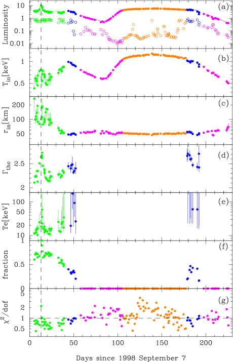
Figure 5: Same as Fig. 3, but based on the three component model fits to the PCA+HEXTE data (§4.2). The data points after day 52 are the same as in Fig. 3. (a)Time history of $L_{\rm disk}+L_{\rm thc}$ is plotted with filled circle instead of $L_{\rm disk}$ for the very high state data, where $L_{\rm thc}$ is estimated under an assumption of isotropic emission. (b)–(f) Those of $T_{\rm in}$, $r_{\rm in}$, $T_{\rm e}$, $\Gamma_{\rm thc}$, $L_{\rm thc}/(L_{\rm disk}+L_{\rm thc})$, and $\chi^{2}/{\rm dof}$, respectively. Panels (a) and (c) are based on the normalization factor obtained with the PCA data.

5 Simultaneous ASCA-PCA-HEXTE data

One obvious caveat of the spectral modelling is that the low temperatures inferred for the strong very high state mean that the disc spectrum is not well covered by the PCA bandpass which starts only at $\sim$3 keV. Hence we use the simultaneous ASCA GIS data to extend the soft energy response. We use the same three continuum component model and fitting conditions as above, except that the value of $N_{\rm H}$ is now a free parameter. Same as in §4.2, except for a normalization factor, all the model parameters are constrained to be the same between the GIS, the PCA and the HEXTE data. Table 3 shows the fitting results. Figure 8 shows the raw data and the residuals between the data and the model, and Fig. 8 shows an unfolded spectrum with the model. The model fits the simultaneous data very well with $\chi^{2}/{\rm dof}=150.4/186$. The best fit value of $T_{\rm in}=0.54\pm 0.02$ keV is much more tightly constrained, and its central value is slightly shifted to lower temperature than $0.65^{+0.08}_{-0.04}$ keV derived from the RXTE data alone.

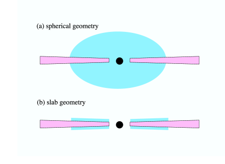
Figure 6: Schematic pictures of assumed geometries of the corona. Spherical(a) and slab(b) geometries are shown.

In order to check the results with a more physical model, we replace the phenomenological line and smeared edge spectral features with the full reflection code included in the thcomp model (Zycki, Done & Smith 1998). We fix the inclination and iron abundance at $70^{\circ}$ and solar abundance, respectively. These fit results are shown as model (b) in Table 3. The derived reflection parameters look somewhat unphysical, with a large amount of mostly neutral reflection. This is probably due to limitations of the reflection modelling for an ionized disc in thcomp, which is based on the pexriv reflected continuum calculations (Magzdiarz & Zdziarski 1995). These codes calculate the ionisation balance in a very simplistic way (Done et al. 1992), assumming it to be constant throughout the disc rather than varying as a function of height (Nayakshin et al. 2000; Ballantyne, Ross & Fabian 2001).

Another issue is that these models assume that Compton upscattering is negligible below 12 keV. However, for ionised material this can be very important in determining the iron line and edge structure observed (Ross, Fabian & Young 1999). While more accurate ionised reflection models are available for spectral fitting (Nayakshin et al. 2000; Ballantyne, Iwasawa & Ross 2001), they assume a very simple continuum form (power law, or power law with exponential cutoff) which means they cannot accurately describe the complex spectral shape observed in these very high state data. Instead, we estimate the impact of this uncertainty in the reflection modelling by removing the iron line and edge region (5–12 keV) and refitting the data with the thcomp reflected continuum with an ionization parameter, $\xi$, fixed at $10^{2}$, $10^{3}$ and $10^{4}$, (models (c), (d) and (e) respectively in Table 2).

The disc luminosities and temperatures derived from the series of models (a–e in Table 2) are plotted as filled black squares on the $T-L$ plots (Fig. 4b–d). These show the range of systematic uncertainties present from the spectral modelling. However, all of the fits detailed in Table 2 have an even lower disc temperature than that derived from fits to the PCA+HEXTE data, but with a similar luminosity. These show even more clearly that the strongly Comptonised spectra are not easily consistent with an untruncated disc. For the simple corona geometries of Fig. 6, then in order to explain the high inferred intrinsic disc luminosity, $L_{\rm disk}^{\rm int}\sim 2$–$3\times 10^{38}~{}{\rm erg~{}s^{-1}}$, with the same disc radius as seen in the standard high/soft state requires $T_{\rm in}>$ 0.85–0.9 keV. By contrast, the 99.9% upper limits ($\chi^{2}/{\rm dof}=1.35$ for dof of 186–188) of the disc temperature from the ASCA-PCA-HEXTE data is $<0.66$ keV for all the models (a–e) in Table 2. Fixing $T_{\rm in}=0.85$ keV results in completely unacceptable fits ($\chi^{2}/\rm dof$ =4.6–5.6).

More conservatively, even when the systematic errors of the PCA data and the HEXTE data increased to 1 %, the 99.9 % upper limit is still lower than 0.69 keV. Since deviations between the modeled and measured Crab spectrum do not exceed 1 % as noticed by many authors including Revnivtsev et al.  (2003), $T_{\rm in}=0.69$ keV can be considered as the securest upper limit of the disc inner temperature. It is clear that the low disc temperature derived in the strong very high state spectra from the PCA+HEXTE fits are not due to lack of PCA coverage of the disc spectrum, or the spectral modelling of the reflection emission.

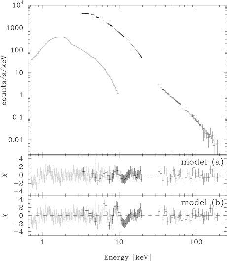
Figure 7: The simultaneous spectral fit on GIS, PCA and HEXTE, with the best fit model predictions.

Figure 8: Unfolded spectrum of Fig. 8 with the predictions of model (a).

6 Discussion

We have shown that the strong very high state spectra really do have a rather low temperature disc for its luminosity. These observations suggest that the disc is truncated at larger radii than the last stable orbit in the strong very high state. However, this is based on the assumptions that (1) the correction factor of color to effective temperature is kept approximately constant, and (2) the corona fully covers the disc as illustrated in Fig. 6

6.1 Change of color temperature correction

Figure 5c represents the time history of the apparent inner radius $r_{\rm in}$, as derived from the temperature and luminosity values given in Fig. 4d. The true inner radius $R_{\rm in}$ is related to $r_{\rm in}$ as $R_{\rm in}\propto\kappa^{2}r_{\rm in}$, where $\kappa$ is the colour temperature correction. For constant $\kappa$, the observed variability of $r_{\rm in}$ is just caused by change of the inner radius. However, a change in the colour temperature correction could be expected as a function of disc luminosity (Merloni et al. 2000; GD04; Kawaguichi 2003), and illumination of the upper layers of the disc (Nayakshin et al. 2000) and/or conductive heating could also lead to an increase in $\kappa$.

Close inspection of Fig. 4d shows that the data points corresponding to the weak very high state (anomalous regime) are slightly lower than the solid line denoting constant $r_{\rm in}$. Although this is not very significant, it could perhaps indicate a constant radius disc with slightly higher colour temperature correction. Conversely, the disc in the strong very high state requires a decrease in colour temperature correction by a factor of $\sim 60$% i.e. $\kappa\sim 1$. This would imply that the observed colour temperature was the same as the effective disc temperature, which is only possible when true absorption opacity dominates over electron scattering. This cannot be the case at the observed $\sim$0.5 keV temperatures. Changing $\kappa$ cannot explain the strong very high state spectra with the disc with a constant radius.

The above discussion assumed that the disc spectrum can be described by a simple colour temperature correction. Plainly this may not be the case, and the disc spectrum could be completly distorted, for example if the inner disc colour temperature correction were much higher than at outer radii. The spectrum would then look like a low temperature disc with some fraction of the emission at much higher temperature. This is exactly what these strong very high state spectra look like, so we examine the effect of Comptonization as a function of radius on the disc spectrum below.

6.2 Geometry and energetics of the corona

So far, we assumed the corona fully covers the disc as illustrated in Fig. 6. However several other geometries can be considered, as illustrated in Fig. 9. If the corona is out of our line of sight to the disc e.g. a small inner region, perhaps physically representing an inner jet or bulk Comptonisation of the infalling material (see Fig. 9a and b), then the Compton scattering does not affect the observed disc flux, so the correction used above overestimates the intrinsic disc emission. The problem of such a geometry is that the Comptonising region would see many fewer disc photons than an observer, in conflict with the data (see Tables 2 and 3). Even without this problem, the best that such a geometry could do is reduce the estimated intrinsic disc luminosity to that observed (i.e. where none of the disc photons in our line of sight are intercepted). This puts us straight back to Fig. 4b, where the ASCA+PCA+HEXTE data show a much lower temperature disc than expected for its luminosity in the very high state.

Alternatively, the corona could be patchy (Fig. 9c), or cover only the inner disc (Fig. 9d). In both these geometries the corona is in the line of sight to the disc, so again this predicts that the Compton scattered photons we see are removed from the observed disc emission. The intrinsic disc emission should still be estimated as in Fig. 4d. While the patchy corona could take photons uniformly from the whole disc, the inner corona (Fig. 9d) would preferentially take only the inner disc (highest temperature) photons, perhaps leading to an underestimate of the disc temperature. This is analogous to having a variable colour temperature correction with radius (see above). We model this by switching the seed photons in thcomp to blackbody (rather than the MCD), and allow the temperatures of the observed inner disc and seed photons to be different. This gives a very strong upper limit on the seed photon temperature for the ASCA-PCA-HEXTE data of $<0.6$ keV, showing that the low disc temperature is not an artifact of the seed photon distribution assumed.

However, the existence of the corona changes the disc temperature structure. In the limit of a corona that covers the whole disc then this has little effect as both the disc luminosity and temperature are reduced (Svensson & Zdziarski 1994), but for an inner disc corona the behaviour is more complex. Only the inner disc temperature and luminosity are reduced, but these form the seed photons for the Compton scattering. For a fraction $f$ of the total accretion power dissipated in the corona, the inner disc temperature is reduced by a factor $(1-f)^{1/4}$ (Svensson & Zdziarski 1994). This is an underestimate of the inner disc temperature as it intercepts and reprocesses a large fraction (up to a half) of the coronal flux. We will do more detailed modelling of this in a subsequent paper, but estimate that the size of this effect is not enough to make the temperature and luminosity consistent with the standard high/soft state radius disc.

7 A scenario for the disc evolution in the 1998 outburst of XTE J1550-564

7.1 A scenario derived by spectral studies

The discussion above shows that there are no easy alternatives to the conclusion that the inner disc is truncated in the strongly Comptonised very high state spectra. If so, then there must be some overlap between the inner hot region and the truncated disc in order for it to intercept enough seed photons, but the larger radius disc can trivially produce the lower observed disc temperature at high luminosity. This geometry is rather similar to the truncated disc/hot inner flow inferred for the low/hard state, so would give a physical basis for the well known similarities between the very high state spectra and the intermediate state spectra (seen towards the very end of the low/hard state; Belloni et al. 1996; Mendez et al. 1997). It could also explain the lower frequency QPO seen in the very high state (e.g. the review by van der Klis 2000; di Matteo & Psaltis 1999).

A schematic picture for the whole disc evolution during the 1998 outburst of XTE J$1550-564$ is shown in Fig. 10. The outburst starts in the low/hard state, with a truncated disc, and hot inner flow (panel a). The increase in mass accretion rate increases the optical depth of the inner flow before the inner disc has time to form, leading to an optically thick, cooler inner flow and truncated disc (the strongly Comptonised very high state, panel b) on $\sim$day 5 (WD01). During days 5–30, the fraction of energy dissipated in the corona to that from the disc is kept almost constant (Fig. 5f), while $T_{\rm e}$ and $\Gamma_{\rm thc}$ of the corona changed with time (Fig. 5d and e). Through this period, the X-ray flux reached at the peak (day 13). The radio flare was observed at this time with a continuance of 5 days, and VLBA image showed evolving structure (Hannikainen et al.  2001).

During days 30–40 the inner disc is able to form at progressively smaller radii, perhaps due to the correlated decrease in fractional power dissipated in the corona (see Fig. 5f) which reduces the coronal heating/irradiation. The disc finally reaches the last stable orbit at around day 40, causing a noticeable change in disc temperature behaviour despite little change in luminosity (Fig. 5b). The power dissipated in the corona continues to drop, leading to more weakly Comptonised spectra above the untruncated disc (the weak very high state, anomalous regime; days 40-52). This eventually becomes a small ($<$ 20%) fraction of the total power, giving the standard high/soft state (after day 52, panel e). This is similar to the geometry for the spectral states proposed by Esin et al. (1997), except that the strongly Comptonised very high state spectra corresponds here to a truncated disc.

While this gives a good overall description of the properties of XTE J$1550-564$ during its outburst, the remaining problem is what makes the truncated disc with the strong Compton corona. Advection dominated accretion flows cannot be maintained at such high luminosities (e.g. Esin et al. 1997), although these are only an approximation to the complex nature of the optically thin, hot flow which is predicted from numerical simulations (Hawley & Balbus 2002). Physically, such truncation could arise from disc overheating (Beloborodov 1998), or by strong conduction/irradiative heating from the corona, or, perhaps most attractively, by disruption of the inner disc by jet formation. However, the total mass accretion rate cannot be the trigger for this behaviour since (apart from the peak) the very high state spectra have total luminosity which is similar to that in the disc dominated regime seen in days 100–180. Therefore some other parameters are required to drive the structural changes in the disc (see e.g. van der Klis 2001; Homan et al.  2001; MR03)

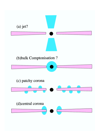
Figure 9: Other candidates of geometries of the material which up-scatters the disc photons.

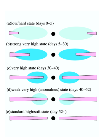
Figure 10: Schematics of obtained picture of the disc evolution on the beginning of the first outburst of XTE J$1550-564$. Panels (a), (d) and (e) refer to pictures of ”Low State”, ”High State” and ”Very High State” in Figure 1 of Esin et al. (1997), respectively.

7.2 Consistency with the QPO behavior

The type of QPO seen is roughly consistent with the changes in geometry shown in Fig. 10, and with the spectral state (Table 1) as suggested by Homan et al.  (2001) based on the spectral hardness ratio. Since the QPO frequencies are thought to reflect the size of the Comptonising region and the disc inner radii, it is meaningful to compare evolution of the QPO frequencies with that of disc inner radii estimated by the spectral analyses. As we can see in Fig. 1, through day 18–30, the frequency of the low-frequency QPO increased from $\sim 2.7$ Hz, and after the day 30, it was almost kept constant at $\sim 6$ Hz. This is very consistent with the decrease in $r_{\rm in}$ derived from the spectra through days 5–40 as shown in Fig. 5c. Indeed, Homan et al.  2001 suggested almost the same scenario of evolution of the accretion disc based on the QPO behavior.

However, there is some inconsistency between the timing and the spectral behavior before day 18. On one hand, the low-frequency QPO increased to $\sim 10$ Hz around the peak (day 13). This frequency is higher than the $\sim 6$ Hz which was observed after days 30–40, suggesting that the disc extends closer to the black hole during the peak. Yet the X-ray spectra imply that the disc extends down to the last stable orbit during days 30–40 and truncates at larger radii during the peak(Fig. 5c). Moreover, the high-frequency QPO which is sometimes seen in the very high state data (Fig. 1) shows rather different behaviour. In Fig. 4, we marked the data points which have high-frequency QPOs with big open diamonds. Some green open squares showed both the characteristics of large inner radius by the spectral fits and the high frequency of the QPOs. Therefore, the QPO and the spectral behavior are not easily consistent, pointing either to a lack of understanding of how QPOs and/or disc spectra relate to the inner radius.

As a brief comment, the strong very high state data with high frequency QPO and the low-frequency QPOs of the higher frequencies may be considered to be relate to the jet ejection. As described in § 4.2, the radio flux was observed to increase suddenly at day 13, the peak of X-ray flux (Wu et al.  2002), and the extending radio jet was reported on day 15 by Hannikainen et al.  (2001). In Fig.4, the data points which show strong radio emission were also marked with big circle plus cross. Thus, the data with high-frequency QPO can be understood to have some relation to the jet ejection.

8 Summary and Conclusions

The disc dominated high/soft state of Galactic black holes can be well modelled by a disc of constant inner radius and colour temperature correction. This most probably indicates that the disc extends down to the innermost stable orbit around the black hole. This is clearly seen in the 1998 outburst of XTE J$1550-564$. However, the strongly comptonised very high state spectra seen at the start of the outburst do not follow this trend. Careful modelling of these spectra show that the disc temperature is somewhat lower than expected for the observed disc luminosity for a constant radius disc. Correcting the disc luminosity for the effects of Compton scattering in a disc-corona geometry make this discrepancy much more marked. We discuss the effects of changing colour temperature corrections, and different geometries, but none of these can convincingly reproduce the observed disc temperatures and luminosities. We will model the effects of a more complex coronal geometry (e.g. one with strong radial gradients in optical depth: Fig. 9d) in a subsequent paper, but the simplest solution is that the inner disc is truncated in the strong very high state.

Acknowledgements

The authors would like to thank an anonymous referee for his/her detailed comments. The present work is supported in part by a Sydney Holgate fellowship in Grey College, University of Durham, JSPS Postdoctoral Fellowship for Young Scientists, and by JSPS grant of No.13304014. A.K. is supported by special postdoctoral researchers program in RIKEN.

References

- [1] Ballantyne D. R., Iwasawa K., Ross R. R., , MNRAS, 2002, MNRAS, 323, 506
- [2] Ballantyne D. R., Ross R. R., Fabian A. C., MNRAS, 2001, MNRAS, 327, 10
- [3] Belloni T. et al. , 1996, ApJ, 472, 107
- [4] Beloborodov A. M., 1998, MNRAS, 297, 739
- [5] Cui W., Zhang S. N., Chen W., Morgan E. H., 1999, ApJ, 512, 43
- [6] di Matteo T., Psaltis D., 1999, ApJ, 526, 101
- [7] Done C., et al. , 1992, ApJ, 395, 275
- [8] Done C., Zycki P., Smith D. A., 2002, MNRAS, 331, 453
- [9] Ebisawa K., Mitsuda K., Hanawa T., 1991, ApJ, 367, 213
- [Ebisawa et al. (1994)] Ebisawa K. et al. , 1994, PASJ, 46, 375
- [10] Esin A., McClintock J., Narayan R. 1997, ApJ, 489, 865
- [11] Gierliski M., Done C. 2003, MNRAS, 342, 1083
- [12] Gierliski M., Done C. 2004, MNRAS, 347, 885 (GD04)
- [13] Gierliski M., Zdziarski, A. Z., et al. , 1999, MNRAS, 309, 496
- [Hannikainen et al. (2001)] Hannikainen D., Campbell-Wilson D., Hunstead R., Mclntyre V., Lovell J., Reynolds J., Tzioumis T., & Wu, K. 2001, AP&SS, 276, 45
- [14] Hawley J. F., Balbus S. A., 2002, ApJ, 573, 736
- [15] Homan J. et al. , 2001, ApJ, 132, 377
- [16] Kawaguchi T., 2003, ApJ, 593, 69
- [17] Kubota A., et al. , 1998, PASJ, 50, 667
- [18] Kubota A., Makishima K., Ebisawa K., 2001, ApJ, 560, L147
- [19] Kubota A., Makishima K., 2004, ApJ, 601, 428 (KM04)
- [20] Magdziarz P., Zdziarski A., 1995, MNRAS, 273, 837
- [] Makishima K., et al. 1996, PASJ, 48, 171
- [21] McClintock J. E., Remillard R. A. 2003, in Compact Stellar X-ray Sources, eds. Lewin W. H. G., & van der Klis, M., (Cambridge University Press, Cambridge), in press (astro-ph/0306213) (MR03)
- [22] Mendez R. H., van der Klis M., 1997, ApJ, 479, 926
- [23] Merloni A., Fabian A. C., Ross R. R., 2000, MNRAS, 313, 193
- [Mitsuda et al. (1984)] Mitsuda K., et al. 1984, PASJ, 36, 741
- [Miyamoto et al. (1991)] Miyamoto S., Kimura K., Kitamoto S., Dotani T., Ebisawa K. 1991, ApJ, 383, 784
- [24] Nayakshin S., Kazanas D., Kallman T. R., 2000, ApJ, 537, 833
- [Orosz et al. (2002)] Orosz J. A. et al. 2002, ApJ, 568, 845
- [Remillard et al. (2002)] Remillard R. A., Sobczak G. J., Muno M. P., McClintock J. E., 2002, ApJ, 564, 962
- [25] Revnivtsev, M., Gilfanov M., Sunyaev R., Jahoda K., Markwardt C. 2003, A&A, 411, 329
- [26] Rothschild R. E. et al. 1998, ApJ, 496, 538
- [27] Ross R. R., Fabian A. C., Young A. J., 1999, 306, 461
- [28] Rybicki G. B., Lightman A. P., 1979, in Radiative process in astrophysics, (John Wiley & Sons, Inc)
- [29] Shakura N., Sunyaev R., 1973, A&A, 24, 337 (SS73)
- [Shimura & Takahara (1995)] Shimura T., Takahara F.,1995, ApJ, 445, 780
- [Smith 1998] Smith, D.A. 1998, IAUC 7008
- [Sobczak et al. (1999)] Sobczak G. J., McClintock J. E., Remillard R. A., Levine A. M., Morgan E. H, Bailyn C. D., Orosz J. A. 1999, ApJ 517, 121
- [Sobczak et al. (2000a)] Sobczak G. J., McClintock J. E., Remillard R. A., Cui W., Levine A. M., Morgan E. H., & Bailyn C. D. 2000a, ApJ, 531, 53
- [Sobczak et al. (2000b)] Sobczak G. J., McClintock J. E., Remillard R. A., Cui W., Levine A. M., Morgan E. H., & Bailyn C. D. 2000b, ApJ, 544, 993
- [30] Svensson R., Zdziarski A. A., 1994, 436, 599
- [31] Tanaka Y., & Lewin W. H. G. 1995, in X-ray Binaries, eds. Lewin W. H. G., van Paradijs J. and van den Heuvel W. P. J., (Cambridge University Press, Cambridge), p126
- [32] Turner N. J., 2004, ApJ, 605, L45
- [33] van der Klis M., 2000, ARA&A, 38, 717
- [Wilson & Done (2001)] Wilson C. D., Done C. 2001, MNRAS, 325, 167
- [Wilson et al. (1998)] Wilson C. A., Harmon B. A., Paciesas W. S., McCollough M. L. 1998, IAUC 7010
- [] Wu K. et al. 2002, ApJ, 565, 1161
- [34] Zdziarski A. A., Johnson W. N., Magdziarz P.,1996, MNRAS, 283, 193
- [35] Zdziarski A. A., Grove J. E., Poutanen J., Rao A. R., Vadawale S. V., 2001, ApJ, 554, 45
- [36] Zycki, P. T., Done, C. & Smith, D. A., 1998, ApJ, 496, 25