Inflation and Precision Cosmology

Abstract

A brief review of inflation is presented. After having demonstrated the generality of the inflationary mechanism, the emphasize is put on its simplest realization, namely the single field slow-roll inflationary scenario. Then, it is shown how, concretely, one can calculate the predictions of a given model of inflation. Finally, a short overview of the most popular models is given and the implications of the recently released WMAP data are briefly (and partially) discussed.

I Introduction

The inflationary scenario inflation has been invented in order to solve and explain some observational facts (isotropy of the Cosmic Microwave Background Radiation–CMBR–, flatness of the space-like sections, etc …) that could not be properly understood in the context of the standard hot Big Bang theory. Therefore, at the beginning of its history, the inflationary scenario was only able to make postdictions but, given the problems of the standard model at that time, this was already a success. However, soon after its advent, it was realized MuChi ; pert that inflation, when combined with quantum mechanics, can also give a very convincing mechanism for structure formation. In particular, for the first time, it was understood how to generate a scale-invariant power spectrum. Therefore, the inflationary mechanism was able to establish a beautiful connection between facts which, before, were considered as independent. However, since the Harisson-Zeldovich was already known to be in agreement with the observations, it could be argued that, somehow, this was again a postdiction. In fact, the inflationary scenario does not predict a scale invariant spectrum but a nearly scale invariant spectrum, the deviations from the scale invariance being linked to the microphysics description of the theory. This constitutes a definite prediction of inflation that can be tested LLMS .

Slightly more than twenty years after the invention of inflation, the situation has recently changed because, thanks to the high accuracy CMBR data obtained, among others, by the WMAP satellite wmap , we can now start to probe the details of the inflationary scenario and check its predictions. The goal of this short review is, after having tried to justify why the inflationary mechanism is generic (section I), to show how, in its most popular and simplest realization, one can calculate concrete predictions (section II) and compare them with the recent observations (section III). These proceedings, due to the lack of space, do not cover many important topics. Among them and since this is particularly relevant for the present article, we just would like to signal the discussion of why the presence of the CMBR Doppler peaks strongly suggests that a phase of inflation took place in the early universe, see Ref. dod .

II The inflationary mechanism

II.1 Basic equations

The cosmological principle implies that the universe is, on large scales, homogeneous and isotropic. This simple assumption drastically constrains the possible shapes of the Universe which can solely be described by the Friedman-Lemaître-Robertson-Walker (FLRW) metric: ${\rm d}s^{2}=-{\rm d}t^{2}+a^{2}(t)\gamma_{ij}^{(3)}{\rm d}x^{i}{\rm d}x^{j}$, where $\gamma_{ij}^{(3)}$ is the metric of the three-dimensional space-like sections of constant curvature. The time-dependent function $a(t)$ is the scale factor. If the spatial curvature vanishes then $\gamma_{ij}^{(3)}=\delta_{ij}$, where $\delta_{ij}$ is the Krönecker symbol. The previous expression is written in terms of the cosmic time $t$ but it is also interesting to work in terms of the conformal time $\eta$ defined by ${\rm d}t=a(\eta){\rm d}\eta$. Then, the metric can be re-expressed as

$${\rm d}s^{2}=a^{2}(\eta)\left[-{\rm d}\eta^{2}+\gamma^{(3)}_{ij}{\rm d}x^{i}{\rm d}x^{j}\right]\,.$$ (1)

In terms of conformal time, the Hubble parameter $H=\dot{a}/a$ can be written as $H={\cal H}/a$ where ${\cal H}\equiv a^{\prime}/a$, a dot denoting a derivative with respect to cosmic time while a prime stands for a derivative with respect to conformal time.

The matter is assumed to be a collection of $N$ perfect fluids and, as a consequence, its stress-energy tensor is given by the following expression

$$T_{\mu\nu}=\sum_{i=1}^{N}T_{\mu\nu}^{(i)}=(\rho+p)u_{\mu}u_{\nu}+pg_{\mu\nu}\,,$$ (2)

where $\rho$ is the (total) energy density and $p$ the (total) pressure. These two quantities are linked by the equation of state, $p=\omega(\rho)$ [in general, there is an equation of state per fluid considered, i.e. $p_{i}=\omega_{i}(\rho_{i})$]. The vector $u_{\mu}$ is the four velocity common to all fluids and satisfies the relation $u_{\mu}u^{\mu}=-1$. In terms of cosmic time this means that $u^{\mu}=(1,0)$ whereas in terms of conformal time one has $u^{\mu}=(1/a,0)$ and $u_{\mu}=(-a,0)$. The fact that the stress-energy tensor is conserved, $\nabla^{\alpha}T_{\alpha\mu}=0$, implies $\rho^{\prime}+3{\cal H}(\rho+p)=0$. This expression is obtained from the time-time component of the conservation equation. The time-space and space-space components do not lead to any interesting equations for the background.

We are now in a position to write down the Einstein equations which are just differential equations determining the scale factor. In terms of cosmic time, they read

$$\frac{\dot{a}^{2}}{a^{2}}+\frac{k}{a^{2}}=\frac{\kappa}{3}\rho\,,\quad-\biggl{(}2\frac{\ddot{a}}{a}+\frac{\dot{a}^{2}}{a^{2}}+\frac{k}{a^{2}}\biggr{)}=\kappa p\,,$$ (3)

where $\kappa\equiv 8\pi G=8\pi/m_{{}_{\mathrm{Pl}}}^{2}$, $m_{{}_{\mathrm{Pl}}}$ being the Planck mass and where $k=0,\pm 1$ is the normalized three-dimensional curvature. Combining the two expressions above, one obtains an equation which permits to express the acceleration of the scale factor $\ddot{a}/a=\kappa(\rho+3p)/6$. From the above equation, one sees that any form of matter such that $\rho+3p<0$ will cause an acceleration of the scale factor (this is only true, of course, if the matter component satisfying $\rho+3p<0$ is the dominant one). The energy density is always positive but, in some situation, the pressure can be negative and the inequality $\rho+3p<0$ may be realized. This simple remark is at the heart of the inflationary scenario. Let us notice that the above property is deeply rooted into the fundamental principles of general relativity. It is because all forms of energy weighs in general relativity that the pressure participates to the equation giving the expression of $\ddot{a}$. This has to be contrasted with Newtonian physics where the same expression reads $\ddot{a}/a=-\kappa\rho/6$, i.e. only the energy density affects the expansion. As a consequence, the expansion can only be decelerated.

A class of solutions of particular interest is that for which the equation of state $\omega\equiv p/\rho$ is a constant. In this case, the conservation equation can be immediately integrated and leads to $\rho\propto a^{-3(1+\omega)}$. Then, the scale factor is given by a power law either of the conformal or of the cosmic time, namely

$$a(\eta)=\ell_{{}_{0}}|\eta|^{1+\beta},\quad a(t)=a_{{}_{0}}\biggl{|}\frac{t}{t_{{}_{0}}}\biggr{|}^{p}\,,$$ (4)

where the sign of the conformal and cosmic times, to be discussed below, can be negative or positive. The parameters $p$ and $\beta$ are related by $\beta=(2p-1)/(1-p)$ and $p=(1+\beta)/(2+\beta)$. The link between $\omega$ and the parameters $\beta$ and $p$ can be expressed as

$$\omega=\frac{1-\beta}{3(1+\beta)}=-1+\frac{2}{3p}\,.$$ (5)

The cases $\beta=-1$ and/or $p=0$ are obviously meaningless since they do not correspond to a dynamical scale factor.

Let us now come back to the question of the sign of the conformal and cosmic times. For the class of models under consideration, the Hubble parameter can be easily calculated and is given by $H=p/t$. Let us first consider the case where we have an expansion, i.e. $H>0$. In this case, one has $t>0$ for $p>0$ and $t<0$ for $p<0$. On the other hand, in the case of a contraction, $H<0$, we have $t>0$ for $p<0$ and $t<0$ for $p>0$. The link between the two times, ${\rm d}t=a{\rm d}\eta$, takes the form

$$\eta = \frac{1}{a_{{}_{0}}(1-p)}|t|^{1-p},\quad\mbox{if}\quad t>0\,,$$ (6)

$$\eta = \frac{-1}{a_{{}_{0}}(1-p)}|t|^{1-p},\quad\mbox{if}\quad t<0\,,$$ (7)

from which we deduce that, if $t>0$, then $\eta<0$ for $p>1$ and $\eta>0$ for $p<1$ and that, if $t<0$, then $\eta>0$ for $p>1$ and $\eta<0$ for $p<1$.

Finally, let us also examine some cases of particular interest. The case $p=2/3$ corresponds to an expanding matter dominated universe and $\omega=0$. Therefore, we have $\eta>0$ and $t>0$. The same conclusion applies for the case $p=1/2$, i.e. the case of an expanding radiation dominated universe with $\omega=1/3$. The case $\beta=-2$ corresponds to $p=\infty$, that is to say to an exponential scale factor: this is just the de Sitter solution with $\omega=-1$. For $\beta<-2$, one has $p>1$ and $\eta<0$, $t>0$ if we are interested in the case of expansion.

The evolution of the background space-time can be very roughly understood by means of the previous set of simple equations. The hot Big Bang model before the advent of inflation just consisted into a radiation dominated epoch ($\omega=1/3$) taking place at high redshifts, until $z_{\rm eq}\simeq 10^{4}$, followed by a phase dominated by cold matter ($\omega=0$). However, already at this level, this very simple framework leads to unacceptable conclusions. We now describe what are (some of) the problems of the pre-inflationary hot Big Bang scenario and how postulating a new phase of accelerated expansion in the very early universe can avoid these problems.

II.2 The horizon problem

The horizon problem consists in the following. The furthest event that we can directly “see” in the universe is the (re)combination, i.e. the time at which the electrons and the protons combined to form hydrogen atoms. Since the photon–atom cross-section (Rayleigh cross-section) is much smaller than the photon–electron cross-section (Thomson cross-section), the universe became transparent at that time. The COBE cobe and WMAP wmap maps of the sky are photographs of the universe at this epoch. The recombination took place at a redshift of $z_{\rm lss}\simeq 1100$, i.e. within the epoch dominated by the cold matter. Before, the universe was opaque and therefore it is not possible to observe it directly at earlier times from the Earth. Since no physical process can act on scales larger than the horizon (see below for a precise definition of the horizon), we typically expect the universe to be strongly inhomogeneous on those scales. Seen from the Earth, this means that the COBE map should look extremely different on angular scales larger than the angular scale of the horizon at recombination.

In order to investigate the consequences of the above statement, let us calculate the angular diameter of the horizon at recombination, seen by an observer today. Roughly speaking, this is just the size of the horizon at the last scattering surface divided by the present (angular) distance to the last scattering surface. In other words, it can be expressed as $\Delta\Omega=d_{{}_{\rm H}}(t_{\rm lss})/d_{{}_{\rm A}}(t_{\rm lss})$, where we now discuss precisely the meaning of the terms in the above formula.

For this purpose, it is convenient to choose the coordinates system such that the origin is located on Earth, i.e. such that “our” co-moving coordinate is $r=0$. Suppose that a photon is emitted at spatial co-moving coordinates $(r_{\rm em},\theta_{\rm em},\varphi_{\rm em})$ and at cosmic time $t_{\rm em}$. The path followed by the photon can be chosen such that $\theta=\mbox{cst}.$ and $\varphi=\mbox{cst}$ since this is a solution of the geodesic equation. In this case, the path is completely characterized by the function $r=r(t)$. This quantity is given by

$$r(t)=r_{\rm em}-\int_{t_{\rm em}}^{t}\frac{{\rm d}\tau}{a(\tau)}\Rightarrow d_{{}_{\rm P}}(t)=a(t)\biggl{[}r_{\rm em}-\int_{t_{\rm em}}^{t}\frac{{\rm d}\tau}{a(\tau)}\biggr{]}\,,$$ (8)

where $d_{{}_{\rm P}}(t)$ is the physical (proper) distance from the “position” of the photon at time $t$ to the origin.

This equation can be used to define the horizon. Indeed, the question that one may ask is the following. At a given (reception) time, $t=t_{\rm rec}$, what is the proper distance to the furthest point where a photon, sent to us from there, could have reached the Earth (the point of co-moving coordinate $r=0$) before or at the time $t_{\rm rec}$? This proper distance is called the size of the horizon at time $t=t_{\rm rec}$. Clearly the distance is maximized if the time of emission is the Big-Bang and if the photon has just reached the Earth at the time $t_{\rm rec}$. Hence the co-moving coordinate of emission is obtained by writing that $d_{{}_{\rm P}}(t_{\rm rec})=0$ and by taking a vanishing lower bound in the previous integral. This implies that

$$r_{\rm em}=\int_{0}^{t_{\rm rec}}\frac{{\rm d}\tau}{a(\tau)}\,.$$ (9)

This means that the distance to the horizon, at the time $t=t_{\rm rec}$, is given by $d_{{}_{\rm H}}(t_{\rm rec})=a(t_{\rm rec})r_{\rm em}$. In this equation, $t_{\rm rec}$ can be for instance the time of recombination, $t_{\rm lss}$ or the present time $t_{0}$ depending on whether one wants the evaluate the size of horizon at the last scattering surface or now.

Another question is to calculate the distance to a point where a photon emitted at $t=t_{\rm em}$ has just arrived on Earth now, at time $t=t_{0}$. Writing again that the photon is received now, one obtains the corresponding co-moving coordinate of emission $r_{\rm em}=\int_{t_{\rm em}}^{t_{0}}{\rm d}\tau/a(\tau)$. From the previous equation, one can deduce that the corresponding angular distance to the point of emission is given by $d_{{}_{\rm A}}\equiv a(t_{\rm em})r_{\rm em}$. Indeed, the FLRW metric can be written as (for flat space-like section) ${\rm d}s^{2}=-c^{2}{\rm d}t^{2}+a^{2}(t)({\rm d}r^{2}+r^{2}{\rm d}\Omega_{2}^{2})$ and therefore the proper distance $D$ across a source is $D\simeq ar\Delta\Omega$ at time $t_{\rm em}$ (obtained from ${\rm d}t={\rm d}r=0$ since it is supposed that the source is located on a sphere of radius $r=\mbox{cte}$). As a consequence, one has $\Delta\Omega=D/(ar)$ from which we deduce $d_{{}_{\rm A}}\equiv a(t_{\rm em})r(t_{\rm em})$. Notice that the proper distance to the point of emission is $a(t_{0})r_{\rm em}$. For very high redshifts, as for instance $z_{\rm lss}$, these two distances are of course very different.

We can now deduce the general expression of the angular diameter. It is given by

$$\Delta\Omega=\biggl{[}\int_{0}^{t_{\rm lss}}\frac{{\rm d}\tau}{a(\tau)}\biggr{]}\times\biggl{[}\int_{t_{\rm lss}}^{t_{0}}\frac{{\rm d}\tau}{a(\tau)}\biggr{]}^{-1}\,.$$ (10)

In the previous expression, the factors $a(t_{\rm lss})$ have canceled out.

Let us now try to evaluate the above solid angle in a realistic case where matter and radiation are present Ellis . For simplicity, we assume that the universe is radiation dominated before recombination and matter dominated after. In reality, as already mentioned, equivalence between radiation and matter takes place before the recombination but this does not introduce important corrections. Since we are going to study the influence of a phase of inflation, we also assume that the epoch dominated by radiation can be interrupted during the period $t_{\rm i}<t<t_{\rm end}$. During this interval, we assume that the universe is dominated by an unknown fluid the equation of state of which is constant and given by $\omega_{{}_{\rm X}}$. To recover the standard hot Big Bang case, where this epoch does not occur, it is sufficient to consider that $t_{\rm i}=t_{\rm end}$, i.e. to switch off the phase dominated by the unknown fluid. The scale factor is not known exactly but its piecewise expression reads:

$$a(t) = a_{\rm i}(2H_{\rm i}t)^{1/2}\,,\quad 0\leq t<t_{\rm i}\,,\quad a(t)=a_{\rm i}\biggl{[}\frac{3}{2}(1+\omega_{{}_{\rm X}})H_{\rm i}(t-t_{\rm i})+1\biggr{]}^{2/[3(1+\omega_{{}_{\rm X}})]}\,,\quad t_{\rm i}\leq t<t_{\rm end}\,,$$ (11)

$$a(t) = a_{\rm end}[2H_{\rm end}(t-t_{\rm end})+1]^{1/2}\,,\quad t_{\rm end}\leq t<t_{\rm eq}\,,\quad a(t)=a_{\rm eq}\biggl{[}\frac{3H_{\rm eq}}{2}(t-t_{\rm eq})+1\biggr{]}^{2/3},\quad t_{\rm eq}\leq t<t_{0}\,.$$ (12)

At each transitions, the scale factor and its first time derivative are continuous. A straightforward calculation leads to the expressions of the horizon at decoupling and of the angular distance to the last scattering surface. One finds

$$d_{{}_{\rm A}}(t_{\rm lss}) = a_{\rm lss}\int_{t_{\rm lss}}^{t_{0}}\frac{{\rm d}\tau}{a(\tau)}=a_{\rm lss}\times\frac{2}{a_{0}H_{0}}\left[1-\biggl{(}\frac{a_{\rm lss}}{a_{0}}\biggr{)}^{1/2}\right]\,,$$ (13)

$$d_{{}_{\rm H}}(t_{\rm lss}) = a_{\rm lss}\int_{0}^{t_{\rm lss}}\frac{{\rm d}\tau}{a(\tau)}=a_{\rm lss}\times\frac{1}{a_{0}H_{0}}\biggl{(}\frac{a_{\rm lss}}{a_{0}}\biggr{)}^{1/2}\left\{1+\frac{1-3\omega_{{}_{\rm X}}}{1+3\omega_{{}_{\rm X}}}\frac{a_{\rm end}}{a_{\rm lss}}\left[1-\biggl{(}\frac{a_{\rm i}}{a_{\rm end}}\biggr{)}^{(1+3\omega_{{}_{\rm X}})/2}\right]\right\}\,.$$ (14)

From the aboves equations, we deduce the expression of the solid angle

$$\Delta\Omega=\frac{1}{2}\biggl{[}1-(1+z_{\rm lss})^{-1/2}\biggr{]}^{-1}(1+z_{\rm lss})^{-1/2}\biggl{\{}1+\frac{1-3\omega_{{}_{\rm X}}}{1+3\omega_{{}_{\rm X}}}\frac{1+z_{\rm lss}}{1+z_{\rm end}}\biggl{[}1-{\rm e}^{-N(1+3\omega_{{}_{\rm X}})/2}\biggl{]}\biggr{\}}\,,$$ (15)

where $N\equiv\ln(a_{\rm end}/a_{\rm i})$ is the number of ${\rm e}$-foldings during inflation and $z_{\rm end}$ is the redshift at which inflation stops (corresponding to $t=t_{\rm end}$).

Let us first suppose that there is no phase of inflation, i.e. $N=0$. Then, $\Delta\Omega\simeq 0.5\times(1+z_{\rm lss})^{-1/2}\simeq 0.85^{\circ}$.

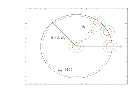
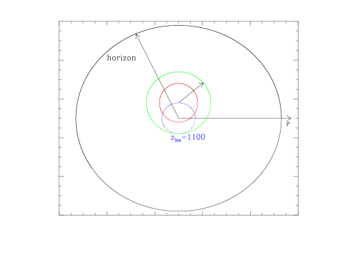
Figure 1: Left panel: Sketch of the evolution of the horizon. The origin of the coordinates is chosen to be Earth. The red circles represent the size of the horizon at the time of equality, $z_{\rm eq}\simeq 10^{4}$. The green circles represent the horizon at the time of recombination $z_{\rm rec}\simeq 1100$. The black circle represents the horizon today. The dotted blue circle represents the surface of last scattering viewed from Earth. The angle $\Delta\Omega$ is the angular size of the horizon at recombination viewed from Earth. Right panel: Sketch of the evolution of the horizon in an inflationary universe. The conventions are the same as in the left panel. The horizon at recombination now includes the last scattering surface and there is no horizon problem anymore

As a consequence, one expects the last scattering surface to be made of $\simeq 1^{\circ}$ patches whose physical properties are completely different (let us remind that the angular diameter of the moon seen from the Earth is $\simeq 0.5^{\circ}$). This is obviously not the case: up to tiny fluctuations of order $\delta T/T\simeq 10^{-5}$, the CMB radiation is extremely homogeneous and isotropic. This paradox is called the horizon problem. A solution to this problem is to assume that the initial conditions were identical in all the causally disconnected patches but this seems very difficult to justify. Another solution is to switch on the inflationary phase. To significantly modify the solid angle in Eq. (15), the unknown fluid responsible for inflation must have an equation of state such that $\omega_{{}_{\rm X}}<-1/3$. Indeed, if $1+3\omega_{{}_{\rm X}}>0$, then the argument of the exponential in Eq. (15) is negative and the correction coming from the phase driven by the unknown fluid becomes negligible. On the other hand, if $1+3\omega_{{}_{\rm X}}<0$, then the correction can be very important, depending of course on the value of the number of e-folds $N$. Writing that the last scattering surface looks very isotropic, that is to say $\Delta\Omega>4\pi$, allows us to put a constraint on this quantity. One obtains $N\gtrsim-4+\ln z_{\rm end}$. Notice that it is necessary to assume that $\omega_{{}_{\rm X}}$ is not too close to $-1/3$ otherwise terms like $1+3\omega_{{}_{\rm X}}$, that we have neglected, could also have an effect on the constraint derived above.

Let us now try to better understand and to physically interpret what has been done. This is summarized in Fig. 1 that we now describe in more details. The proper distance to the last scattering surface is given by

$$d_{\rm lss}=a_{0}\int_{t_{\rm lss}}^{t_{0}}\frac{{\rm d}\tau}{a(\tau)}=\frac{2}{H_{0}}\left[1-\biggl{(}\frac{a_{\rm lss}}{a_{0}}\biggr{)}^{1/2}\right]\,.$$ (16)

This is approximatively the Hubble distance today, defined by $\ell_{{}_{\rm H}}\equiv H_{0}^{-1}$, since we have $d_{\rm lss}\simeq 2H_{0}^{-1}\simeq 6000h^{-1}\mbox{Mpc}\simeq{\cal O}(1)\ell_{{}_{\rm H}}$ where we have used $H_{0}\equiv 100h\mbox{km}\,\mbox{s}^{-1}\mbox{Mpc}^{-1}$. Obviously, this number does not depend on the fact that there is a phase of inflation or not. On the other hand, the size of the horizon today is given by the following expression

$$d_{{}_{\rm H}}(t_{0})=a_{0}\int_{0}^{t_{0}}\frac{{\rm d}\tau}{a(\tau)} = a_{0}\times\frac{1}{a_{0}H_{0}}\biggl{(}\frac{a_{\rm lss}}{a_{0}}\biggr{)}^{1/2}\left\{1+\frac{1-3\omega_{{}_{\rm X}}}{1+3\omega_{{}_{\rm X}}}\frac{a_{\rm end}}{a_{\rm lss}}\left[1-\left(\frac{a_{\rm i}}{a_{\rm end}}\right)^{(1+3\omega_{{}_{\rm X}})/2}\right]\right\}$$ (17)

$$+a_{0}\times\frac{2}{a_{0}H_{0}}\left[1-\left(\frac{a_{\rm lss}}{a_{0}}\right)^{1/2}\right]\,.$$

If there is no phase of inflation (or if $1+3\omega_{{}_{\rm X}}>0$) then one has $d_{{}_{\rm H}}(t_{0})\simeq 2H_{0}^{-1}\simeq d_{\rm lss}\simeq\ell_{{}_{\rm H}}$. This is why, in the left panel in Fig. 1, the (black) horizon and the (blue) last scattering surface have about the same size. The horizon at recombination has been calculated in Eq. (14). If there is no phase of inflation then one has $d_{{}_{\rm H}}(t_{\rm lss})\simeq H_{0}^{-1}(1+z_{\rm lss})^{-3/2}\ll d_{\rm lss}$. This is why in the left panel in Fig. 1, the red and the green circles are small in comparison with the blue circle representing the last scattering surface. This is also the heart of the horizon problem: without a phase of inflation, the horizon at recombination is too small in comparison with the last scattering surface and, as a consequence, its angular size is only $\simeq 1^{\circ}$ as we have calculated previously.

Let us now turn to the inflationary solution and the right panel in Fig. 1. The proper distance to the last scattering surface is not modified. But, and this is the crucial point, the size of the horizon is now completely different. Using Eq. (14), with now $1+3\omega_{{}_{\rm X}}<0$, we obtain

$$d_{{}_{\rm H}}(t_{\rm lss})\simeq\frac{1}{H_{0}}(1+z_{\rm lss})^{-3/2}\left[1+\frac{z_{\rm lss}}{z_{\rm end}}\left(\frac{a_{\rm end}}{a_{\rm i}}\right)\right]\gg d_{\rm lss}\,.$$ (18)

This is why in the right panel in Fig. 1 the (green) horizon now encompasses the (blue) last scattering surface. Another consequence is that the (black) horizon today is now much bigger than the Hubble scale which, as already mentioned, is still approximatively equal to the size of the blue last scattering surface. For the purpose of illustration let us take the example of chaotic inflation. In this case we have $z_{\rm end}\simeq 10^{28}$ and $a_{\rm end}/a_{\rm i}\simeq\exp(10^{28})$ from which we deduce that (!) $d_{{}_{\rm H}}(t_{0})\simeq 3\times 10^{43429421}h^{-1}\mbox{Mpc}$. Clearly this scale is totally different from the Hubble scale and, in the context of an inflationary universe, one should carefully make the difference between those two scales.

II.3 The flatness problem

This problem becomes more apparent if the Friedman equation is cast into a different form. Let us define the parameter $\Omega_{\rm i}$, which gives the relative contribution of the fluid “i” to the total amount of energy density present in the Universe, by $\Omega_{\rm i}(t)\equiv\rho_{\rm i}(t)/\rho_{\rm cri}(t)$, where the critical energy density is $\rho_{\rm cri}\equiv 3H^{2}/\kappa$. This last quantity is nothing but the total energy density of a universe with flat space-like sections. This is a time-dependent quantity. The Friedman equation takes the form $k/(a^{2}H^{2})=\sum_{i=1}^{N}\Omega_{i}(t)-1\equiv\Omega_{{}_{\rm T}}(t)-1$. The parameter $\Omega_{{}_{\rm T}}(t)$ directly gives the sign of the curvature of the space-like sections. Since $k$ is not a function of time, the sign of $\Omega_{{}_{\rm T}}-1$ cannot change during the cosmic evolution. In general, it is difficult to solve the differential equation giving the time evolution of $\Omega_{{}_{\rm T}}$(t) and to obtain the explicit time dependence of $\Omega_{{}_{\rm T}}$. However, it is possible to express $\Omega_{{}_{\rm T}}$ in terms of the scale factor $a(t)$, at least in the case where all the fluids have a constant equation of state parameter. One obtains

$$\Omega_{{}_{\rm T}}(a)=\sum_{i=1}^{N}\Omega_{i}(t_{0})\left(\frac{a}{a_{0}}\right)^{-3(1+\omega_{i})}\left\{\sum_{\rm j=1}^{N}\Omega_{j}(t_{0})\left(\frac{a}{a_{0}}\right)^{-3(1+\omega_{j})}-\left[\Omega_{{}_{\rm T}}(t_{0})-1\right]\left(\frac{a}{a_{0}}\right)^{-2}\right\}^{-1}\,.$$ (19)

If one assumes that only radiation and matter are present then, as $a/a_{0}$ goes to zero, it is clear that radiation becomes dominant. In this case, a good approximation of the previous equation is

$$\Omega_{{}_{\rm T}}(t)-1\simeq\frac{\Omega_{{}_{\rm T}}(t_{0})-1}{\Omega_{\rm rad}(t_{0})}\biggl{(}\frac{a}{a_{0}}\biggr{)}^{2}=\frac{\Omega_{{}_{\rm T}}(t_{0})-1}{\Omega_{\rm rad}(t_{0})}\biggl{(}\frac{1}{z+1}\biggr{)}^{2}\,.$$ (20)

Today it is known that $|\Omega_{{}_{\rm T}}(t_{0})-1|<0.1$. This clearly means that, at high redshifts, the quantity $|\Omega_{{}_{\rm T}}(z)-1|$ was extremely close to zero. For instance, at the redshift of nucleosynthesis, $z_{\rm nuc}\simeq 3\times 10^{8}$, one has $|\Omega_{{}_{\rm T}}(z_{\rm nuc})-1|\simeq{\cal O}(10^{-14})$ where we have taken $\Omega_{\rm rad}(t_{0})\simeq 10^{-4}$. It is difficult to understand why this quantity was so fine-tuned in the early Universe. At Grand Unified Theory (GUT) scale ($z_{{}_{\rm GUT}}\simeq 10^{28}$), the constraint becomes even worse $|\Omega_{{}_{\rm T}}(z_{{}_{\rm GUT}})-1|\simeq{\cal O}(10^{-52})$. To explain this fact, we have two possible solutions: (i) we simply assume that the initial conditions were fine-tuned in the early Universe or (ii) we find a mechanism which automatically produces such a small value at high redshifts. Since, as already mentioned for the horizon problem, the first explanation seems artificial, let us concentrate on the second one. Thus, we assume that, for redshifts $z>z_{\rm end}$, the Universe was dominated by another type of matter, different from matter or radiation. We simply characterize this unknown fluid $X$ by its equation of state $\omega_{{}_{\rm X}}$. The equation of state should be chosen such that, from any reasonable (i.e. not fine-tuned) initial conditions in the very early Universe $z\gg z_{\rm end}$, it automatically produces a $\Omega_{{}_{\rm T}}-1$ close to zero, with the required accuracy at $z=z_{\rm end}$. $\Omega_{{}_{\rm T}}$ can be written as

$$\Omega_{{}_{\rm T}}(a)=\frac{\Omega_{{}_{\rm X}}(a_{\rm i})}{\Omega_{{}_{\rm X}}(a_{\rm i})+\left[1-\Omega_{{}_{\rm T}}(a_{\rm i})\right]\left(\displaystyle{\frac{a}{a_{\rm i}}}\right)^{1+3\omega_{{}_{\rm X}}}}\,,$$ (21)

where $a_{\rm i}$ is the value of the scale factor at some initial redshift $z_{\rm i}$. Since $a_{\rm end}/a_{\rm i}\gg 1$, the condition $\Omega_{{}_{\rm T}}(a_{\rm end})\simeq 1$ is clearly equivalent to $1+3\omega_{{}_{\rm X}}<0$. Then, from any initial conditions at $z=z_{\rm i}$, the value of $\Omega_{{}_{\rm T}}(a_{\rm end})$ will be pushed toward one as long as $X$ dominates. Therefore, one recovers the fact that a fluid with a negative equation of state parameter can solve a problem of the hot Big Bang model. One can even derive the constraint that the parameters describing the epoch dominated by the fluid $X$ must satisfy. If one requires that $\Omega_{{}_{\rm T}}$ has been pushed so close to one during the phase dominated by $X$ that the remaining difference $\Omega_{{}_{\rm T}}-1$ will not sufficiently increased during the radiation and dominated epochs to compensate the first effect and to be distinguishable from zero today, one arrives at [from Eqs. (20) and (21) written at $z=z_{\rm end}$]

$$\biggl{(}\frac{a_{\rm end}}{a_{\rm i}}\biggr{)}^{1+3\omega_{{}_{\rm X}}}={\rm e}^{N\left(1+3\omega_{{}_{\rm X}}\right)}\lesssim 10^{4}\times z_{\rm end}^{-2}\,,$$ (22)

which can also be expressed as $N\gtrsim-4+\ln z_{\rm end}$, where we have assumed for simplicity that $|1+3\omega_{{}_{\rm X}}|={\cal O}(1)$. It is quite remarkable that this constraint be the same as the one derived from the requirement that the horizon problem is solved. To conclude, let us give some numerical examples: for $z_{\rm end}\simeq 10^{10}$, i.e. two orders of magnitude above nucleosynthesis, one has $a_{\rm end}/a_{\rm i}\simeq 10^{8}$ that is to say $\simeq 19$ e-foldings. For $z_{\rm end}\simeq z_{{}_{\rm GUT}}$, one obtains $a_{\rm end}/a_{\rm i}\simeq 10^{26}$, namely $\simeq 60$ e-foldings.

The main lesson of the previous calculations is that, assuming an epoch in the early Universe dominated by a fluid the equation of state parameter of which is negative, provides an elegant way to solve the problems of the standard hot Big Bang model. Here, the important point is that the detailed properties of the unknown fluid and/or its physical nature are unimportant, at least at the background level, provided the equation of state parameter is negative. This makes the inflationary solution quite generic.

II.4 Single scalar field inflation

We have seen in the previous sections that inflation can be caused by any fluid such that $\rho+3p<0$. We now discuss a concrete realization of the inflationary mechanism. Inflation is supposed to take place in the very early universe, at very high energies. At those scales, the fluid description of matter is not expected to hold anymore and (quantum) field theory seems to be the most appropriate way to describe the behavior of matter. The simplest example, compatible with the symmetries of the FLRW metric, is a scalar field $\phi_{{}_{0}}(\eta)$. This field will be called the inflaton in what follows. The corresponding Lagrangian reads

$$S=-\int{\rm d}^{4}x\sqrt{-g}\biggl{[}\frac{1}{2}g^{\mu\nu}\partial_{\mu}\phi_{{}_{0}}\partial_{\nu}\phi_{{}_{0}}+V(\phi_{{}_{0}})\biggr{]}\,,$$ (23)

where $V(\phi_{{}_{0}})$ is the potential, a priori a free function but we will see that, in order to have a successful inflationary phase, its shape must satisfy some constraints. The stress-energy tensor can be written as

$$T_{\mu\nu}=\partial_{\mu}\phi_{{}_{0}}\partial_{\nu}\phi_{{}_{0}}-g_{\mu\nu}\biggl{[}\frac{1}{2}g^{\alpha\beta}\partial_{\alpha}\phi_{{}_{0}}\partial_{\beta}\phi_{{}_{0}}+V(\phi_{{}_{0}})\biggr{]}\,.$$ (24)

From this expression, one sees that the scalar field can also be viewed as a perfect fluid. The energy density and the pressure are defined according to $T^{0}{}_{0}=-\rho$ and $T^{i}{}_{j}=p\delta^{i}{}_{j}$ and read

$$\rho=\frac{1}{2}\frac{(\phi_{{}_{0}}^{\prime})^{2}}{a^{2}}+V(\phi_{{}_{0}}),\quad p=\frac{1}{2}\frac{(\phi_{{}_{0}}^{\prime})^{2}}{a^{2}}-V(\phi_{{}_{0}})\,.$$ (25)

The conservation equation can be obtained by inserting the previous expressions of the energy density and pressure into Eq. (LABEL:conservation). Assuming $\phi_{{}_{0}}^{\prime}\neq 0$, this reproduces the Klein-Gordon equation written in a FLRW background, namely

$$\phi_{{}_{0}}^{\prime\prime}+2\frac{a^{\prime}}{a}\phi_{{}_{0}}^{\prime}+a^{2}\frac{{\rm d}V(\phi_{{}_{0}})}{{\rm d}\phi_{{}_{0}}}=0\,.$$ (26)

As already mentioned before, the other equation of conservation expresses the fact that the scalar field is homogeneous and therefore does not bring any new information. Finally, a comment is in order about the equation of state. In general, there is no simple link between $\rho$ and $p$ except when the kinetic energy dominates the potential energy where $\omega\simeq 1$, i.e. the case of stiff matter or, on the contrary, when the potential energy dominates the kinetic energy for which one obtains $\omega\simeq-1$. This last case is of course the most interesting for our purpose. This shows that inflation corresponds to a regime where the potential energy dominates the kinetic energy: $V(\phi_{{}_{0}})\gg(\phi_{{}_{0}}^{\prime})^{2}$, see Eqs. (25). We also note in passing that an equation of state $p\simeq-\rho$ implies that the energy density of the field will be almost constant during inflation. The fact that the kinetic energy is small during inflation means that the potential should be very flat which is the main requirement for a successful model of inflation if this one is caused by a scalar field.

In general, the equations of motion can be integrated exactly only for a very restricted class of potentials. On the contrary, one would like to able to characterize this motion for any given, sufficiently flat, potentials. To reach this goal, we clearly need a scheme of approximation. Since the kinetic energy to potential energy ratio and the scalar field acceleration to the scalar field velocity ratio are small, this suggests to view these two ratios as parameters in which a systematic expansion is performed. The slow-roll motion of the scalar field is controlled by the three “slow-roll parameters” (at leading order, see e.g. Ref. SL ) defined by:

$$\epsilon\equiv 3\frac{\dot{\phi_{{}_{0}}}^{2}}{2}\left(\frac{\dot{\phi_{{}_{0}}}^{2}}{2}+V\right)^{-1}=-\frac{\dot{H}}{H^{2}}=1-\frac{{\cal H}^{\prime}}{{\cal H}^{2}}\,,\quad\delta\equiv-\frac{\ddot{\phi_{{}_{0}}}}{H\dot{\phi_{{}_{0}}}}=-\frac{\dot{\epsilon}}{2H\epsilon}+\epsilon\ ,\quad\xi\equiv\frac{\dot{\epsilon}-\dot{\delta}}{H}\ .$$ (27)

Some remarks are in order at this point. First of all, we have introduced a third slow-roll parameters, $\xi$. This is necessary if one wants to establish the exact equations of motion of $\epsilon$ and $\delta$. Secondly, the slow-roll conditions are satisfied if $\epsilon$ and $\delta$ are much smaller than one and if $\xi={\cal O}(\epsilon^{2},\delta^{2},\epsilon\delta)$. Since the equations of motion for $\epsilon$ and $\delta$ can be written as:

$$\frac{\dot{\epsilon}}{H}=2\epsilon(\epsilon-\delta)\ ,\quad\frac{\dot{\delta}}{H}=2\epsilon(\epsilon-\delta)-\xi\,,$$ (28)

it is clear that this amounts to consider $\epsilon$ and $\delta$ as constants. This property turns out to be crucial for the calculation of the perturbations. Thirdly, inflation stops when $\epsilon=-\dot{H}/H^{2}=1$. Finally, it is also convenient to re-express the slow-roll parameters in terms of the inflaton potential. One can show that

$$\epsilon\simeq\frac{m_{{}_{\rm Pl}}^{2}}{16\pi}\biggl{(}\frac{V^{\prime}}{V}\biggr{)}^{2},\quad\delta\simeq-\frac{m_{{}_{\rm Pl}}^{2}}{16\pi}\biggl{(}\frac{V^{\prime}}{V}\biggr{)}^{2}+\frac{m_{{}_{\rm Pl}}^{2}}{8\pi}\frac{V^{\prime\prime}}{V}\,,$$ (29)

where, here, a prime means a derivative with respect to the scalar field (as expected, the third slow roll parameter involves the third derivative of the potential). This suggests a new interpretation of the slow-roll approximation: the slow-roll parameters controls the deviation of the inflaton potential from perfect flatness (the case of a cosmological constant) and hence are given by the successive field derivatives of the potential.

Yet another way to see the slow-roll approximation is the following. The perfect slow-low regime is when the inflaton potential is a constant, i.e. is exactly flat. In this case, one has $\epsilon=\delta=0$ and the corresponding solution of the Einstein equations is the de Sitter space-time with the scale factor $a(\eta)\propto|\eta|^{-1}$. Somehow, the slow-roll approximation is an expansion around this solution. To illustrate this point, let us consider the exact equation:

$$\eta=-\int\frac{1}{1-\epsilon}{\rm d}\biggl{(}\frac{1}{{\cal H}}\biggr{)}\,,$$ (30)

which comes directly from the definition of $\epsilon\equiv 1-{\cal H}^{\prime}/{\cal H}^{2}$ written in terms of the conformal time. An integration by parts and the use of the equation of motion of the slow-roll parameter $\epsilon$ allows us to reduce the previous equation to

$$\eta=-\frac{1}{(1-\epsilon){\cal H}}-\int\frac{2\epsilon(\epsilon-\delta)}{(1-\epsilon)^{3}}{\rm d}\biggl{(}\frac{1}{{\cal H}}\biggr{)}\,.$$ (31)

So far, no approximation has been made. At leading order, $\epsilon$ is a constant and the previous equation reduces to $aH\approx-(1+\epsilon)/\eta$. This is equivalent to a scale factor which behaves as $a(\eta)\approx\ell_{{}_{0}}|\eta|^{-1-\epsilon}$. Therefore, the slow-roll approximation consists in slightly modifying the de Sitter expansion by changing the power index in the expression of the scale factor. Interestingly enough, the effective power index (at leading order) only depends on $\epsilon$. We will see that the second slow-roll parameters will show up in the calculation when we consider inflationary cosmological perturbations.

Finally, it is also useful to make use of the set of horizon flow functions, first introduced in Ref. flow . The big advantage of these parameters is that there are defined in terms of the scale factor only and thus do not rely on the fact that inflation is caused by one scalar field. In particular, these parameters could still be used in a multi-fields model of inflation whereas the set introduced previously should be modified. The zeroth horizon flow function is defined by $\epsilon_{{}_{0}}\equiv H(N_{\rm i})/H(N)$, where $N$ is the number of e-folds after an arbitrary initial time. The hierarchy of horizon flow functions is then defined according to

$$\epsilon_{n+1}\equiv\frac{{\rm d}\ln|\epsilon_{n}|}{{\rm d}N},\quad n\geq 0\,.$$ (32)

The link between the horizon flow functions and the set $\{\epsilon,\delta,\xi\}$ can be expressed as

$$\epsilon=\epsilon_{1}\,,\quad\delta=\epsilon_{1}-\frac{1}{2}\epsilon_{2}\,,\quad\xi=\frac{1}{2}\epsilon_{2}\epsilon_{3}\,.$$ (33)

The fact that $\xi$ is of higher order than the two first slow-roll parameters is now obvious which is another advantage of the horizon flow parameters.

III Inflationary cosmological perturbations

III.1 Gauge-invariant formalism

The perturbed line element can be written as MFB :

$${\rm d}s^{2} = a^{2}(\eta)\{-(1-2\phi){\rm d}\eta^{2}+2({\rm\partial}_{i}B){\rm d}x^{i}{\rm d}\eta$$ (34)

$$+[(1-2\psi)\delta_{ij}+2{\rm\partial}_{i}{\rm\partial}_{j}E+h_{ij}]{\rm d}x^{i}{\rm d}x^{j}\}\ .$$

In the above metric, the functions $\phi$, $B$, $\psi$ and $E$ represent the scalar sector whereas the tensor $h_{ij}$, satisfying $h_{i}{}^{i}=h_{ij}{}^{,j}=0$, represents the gravitational waves. There are no vector perturbations because a single scalar field cannot seed rotational perturbations. At the linear level, the two types of perturbations decouple and thus can be treated separately.

The scalar sector suffers from the gauge problem. This means that an infinitesimal transformation of coordinates (i.e. a “gauge transformation”) could mimic a physical deformation of the underlying background space-time and thus could be confused with a physical mode of perturbations. In order to deal with this problem and to retain only the physical modes, one can either fix the gauge or work with gauge invariant quantities. Here, we choose the latter solution. Scalar perturbations of the geometry can be characterized by the gauge-invariant Bardeen potentials $\Phi$ B1 and fluctuations in the scalar field are characterized by the gauge-invariant quantity $\delta\phi^{\rm(gi)}$

$$\Phi = \phi+\frac{1}{a}\left[a\left(B-E^{\prime}\right)\right]^{\prime}\,,$$ (35)

$$\delta\phi^{\rm(gi)} = \delta\phi+\phi_{{{}_{0}}}^{\prime}\left(B-E^{\prime}\right)\,.$$ (36)

We have two gauge invariant quantities but only one degree of freedom since $\Phi$ and $\delta\phi^{\rm(gi)}$ are linked by the perturbed Einstein equations. As a consequence, if $\phi_{{}_{0}}^{\prime}\neq 0$, then the whole problem can be reduced to the study of a single gauge-invariant variable (the so-called Mukhanov-Sasaki variable) defined by MuChi

$$v\equiv a\left[\delta\phi^{\rm(gi)}+\phi_{{}_{0}}^{\prime}\frac{\Phi}{\mathcal{H}}\right]\,.$$ (37)

In fact, it turns out to be more convenient to work with the rescaled variable $\mu_{{}_{\rm S}}$ defined by $\mu_{{}_{\rm S}}\equiv-\sqrt{2\kappa}v$. Density perturbations are also often characterized by the so-called conserved quantity $\zeta$ L ; MS defined by

$$\zeta\equiv\frac{2}{3}\frac{{\cal H}^{-1}\Phi^{\prime}+\Phi}{1+\omega}+\Phi\,.$$ (38)

The quantity $\mu_{{}_{\mathrm{S}}}$ is related to $\zeta$ by $\mu_{{}_{\mathrm{S}}}=-2a\sqrt{\gamma}\zeta$, where $\gamma=1-{\mathcal{H}}^{\prime}/{\mathcal{H}}^{2}$. The background function $\gamma$ reduces to a constant, $(2+\beta)/(1+\beta)$, for power-law scale factors $a(\eta)\propto(-\eta)^{1+\beta}$. In particular, it is zero for the de Sitter space-time since, in this case, $\beta=-2$. The equation of motion of the quantity $\mu_{{}_{\mathrm{S}}}$ reads MFB

$$\mu_{{}_{\mathrm{S}}}^{\prime\prime}+\left[k^{2}-\frac{(a\sqrt{\gamma})^{\prime\prime}}{(a\sqrt{\gamma})}\right]\mu_{{}_{\mathrm{S}}}=0\,,$$ (39)

where $k$ is the co-moving wavenumber of the corresponding Fourier mode. This equation is similar to a Schrödinger time-independent equation where the usual role of the radial coordinate is now played by the conformal time (this is why the name “time-independent Schrödinger equation” is particularly unfortunate in the present context!). The effective potential $U_{{}_{\rm S}}\equiv(a\sqrt{\gamma})^{\prime\prime}/(a\sqrt{\gamma})$ involves the scale factor $a(\eta)$ and its derivative (up to the fourth order) only.

In the tensor sector (which is gauge invariant by definition) we define the quantity $\mu_{{}_{\mathrm{T}}}$ for each mode $k$ according to $h_{ij}=(\mu_{{}_{\mathrm{T}}}/a)Q_{ij}$, where $Q_{ij}$ are the (transverse and traceless) eigentensors of the Laplace operator on the space-like sections. The equation of motion of $\mu_{{}_{\rm T}}$ is given by Gpara :

$$\mu_{{}_{\mathrm{T}}}^{\prime\prime}+\left(k^{2}-\frac{a^{\prime\prime}}{a}\right)\mu_{{}_{\mathrm{T}}}=0\,.$$ (40)

This formula is similar to the equation of motion of density perturbations. The only difference is that the effective potential, $U_{{}_{\rm T}}=a^{\prime\prime}/a$, now involves the derivatives of the scale factor only up to the second order.

Therefore, we have shown that both types of perturbations obey the same type of equation of motion. The “time-independent Schrödinger” equation can also be viewed as the equation of motion of an harmonic oscillator whose frequency explicitly depends on time, namely the equation of a parametric oscillator MS

$$\mu_{{{}_{\mathrm{S}}},{{}_{\mathrm{T}}}}^{\prime\prime}+\omega_{{{}_{\mathrm{S}}},{{}_{\mathrm{T}}}}^{2}(k,\eta)\mu_{{{}_{\mathrm{S}}},{{}_{\mathrm{T}}}}=0,$$ (41)

with $\omega_{{}_{\mathrm{S}}}^{2}=k^{2}-(a\sqrt{\gamma})^{\prime\prime}/(a\sqrt{\gamma})$, $\omega_{{}_{\mathrm{T}}}^{2}=k^{2}-a^{\prime\prime}/a$.

Finally, the mode functions $\mu_{{}_{\rm S,T}}$ are quantities of interest because the power spectra of density perturbations and gravitational waves, which are observables, directly involve them. Explicitly, one has

$$k^{3}P_{\zeta}(k)=\frac{k^{3}}{8\pi^{2}}\biggl{|}\frac{\mu_{{}_{\rm S}}}{a\sqrt{\gamma}}\biggr{|}^{2},\quad k^{3}P_{h}(k)=\frac{2k^{3}}{\pi^{2}}\biggl{|}\frac{\mu_{{}_{\rm T}}}{a}\biggr{|}^{2}.$$ (42)

The spectral indices and their running are defined by the coefficients of Taylor expansions of the power spectra with respect to $\ln k$, evaluated at an arbitrary pivot scale $k_{*}$.

$$n_{{}_{\rm S}}-1\equiv{{\rm d}\ln{\cal P}_{\zeta}\over{\rm d}\ln k}\biggr{|}_{k=k_{*}},\quad n_{{}_{\rm T}}\equiv{{\rm d}\ln{\cal P}_{h}\over{\rm d}\ln k}\biggr{|}_{k=k_{*}}\,,$$ (43)

are the spectral indices. The fact that scale invariance corresponds to $n_{{}_{\rm S}}=1$ for density perturbations and to $n_{{}_{\rm T}}=0$ for gravitational waves has no deep meaning and is just an historical accident. The two following expressions

$$\alpha_{{}_{\rm S}}\equiv{{\rm d}^{2}\ln{\cal P}_{\zeta}\over{\rm d}(\ln k)^{2}}\biggr{|}_{k=k_{*}},\quad\alpha_{{}_{\rm T}}\equiv{{\rm d}^{2}\ln{\cal P}_{h}\over{\rm d}(\ln k)^{2}}\biggr{|}_{k=k_{*}}\,,$$ (44)

define the “running” of these indices. In principle, we could also define the running of the running and so on.

In order to compute $k^{3}P_{\zeta}(k)$ and $k^{3}P_{h}(k)$, one must integrate the equation of motion (41) and specify what the initial conditions are. We now turn to these questions.

III.2 Qualitative behavior of the solutions

The advantage of the previous formulation is that it allows to guess the form of the solutions very easily. It is essentially determined by three scales. Firstly, one has the physical wavelength of a given Fourier mode $\lambda(\eta)=(2\pi/k)a(\eta)$. A second length scale important for the problem is given by the effective potential. To be specific, one has $\ell_{{}_{\rm U}}(\eta)=a(\eta)/\sqrt{U_{{}_{\rm S,T}}(\eta)}$. Finally, a third scale is the Hubble scale whose definition reads $\ell_{{}_{\rm H}}\equiv a^{2}/a^{\prime}$. A priori, the Hubble scale and the potential scale $\ell_{{}_{\rm U}}$ are different.

Let us now investigate how these scales behave in a typical model of slow-roll inflation. For the purpose of illustration, we only consider the scale factor $a(\eta)\propto|\eta|^{-1}$ during inflation since we have seen before that any model of slow-roll inflation can be seen as a small deformation of the de Sitter space-time.

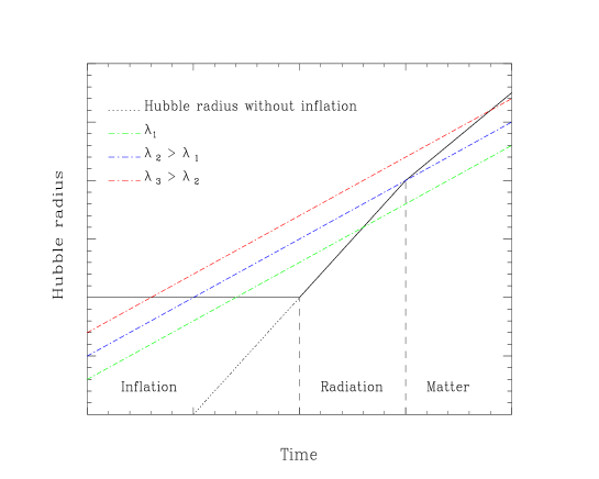
Figure 2: Evolution of the Hubble radius and of three physical wavelengths with different comoving wavenumbers during the inflationary phase and the subsequent radiation and matter dominated epochs. Without inflation, the wavelengths of the mode are super-Hubble initially whereas in the case where inflation takes place, they are sub-Hubble which permits to set up sensible initial conditions.

One immediately obtains that the Hubble radius is constant during inflation while it varies as $\propto a^{2}$ during the radiation era and as $\propto a^{3/2}$ during the matter dominated era. Initially, the physical wavelengths are therefore smaller than the Hubble radius (in principle even smaller than the Planck length, see below) but because of the inflationary expansion of the background they become, at some point, larger than the Hubble radius. The time at which a Fourier mode exits the Hubble radius depends on the co-moving wavenumber of the corresponding mode. They will re-enter the Hubble radius later on, either during the radiation or matter dominated epochs because the Hubble radius behave differently during those eras. It is worth noticing that, without a phase of inflation, the modes would have always been outside the Hubble radius. The fact that there is a regime where the modes are sub-Hubble is therefore a specific feature of the inflationary background and plays a crucial role in our ability to fix well-defined initial conditions. The evolution of a Fourier mode is represented in Fig. 2.

It is also interesting to remark than the physical wavelengths are always inside the horizon which they never exit. It is therefore mandatory to distinguish the horizon from the Hubble scale. In fact it is possible to prove that, as soon as a scale is inside the horizon, it will remain so for ever. This is simply due to the fact that the ratio of the horizon to the physical scale at time $t$ is given by

$$\frac{d_{{}_{\rm H}}}{\lambda}=\frac{k}{2\pi}\int_{t_{\rm i}}^{t_{0}}\frac{{\rm d}\tau}{a(\tau)}+\frac{k}{2\pi}\int_{t_{0}}^{t}\frac{{\rm d}\tau}{a(\tau)}\,,$$ (45)

where $k$ is the co-moving wavenumber of the scale under consideration. The first term is by assumption greater than one and the second one is positive, hence the above-mentioned statement

Looking at the equation of motion, one sees that, a priori, the behavior of the solution is not controlled by the Hubble scale as often said in the literature (sometimes, it is also claimed that the horizon determines the qualitative behavior of the solutions!) but by the scale $\ell_{{}_{\rm U}}$, i.e. by the shape of the effective potential. However, it turns out that, for slow-roll inflation (in fact for power-law inflation), the behaviors of $\ell_{{}_{\rm U}}$ and $\ell_{{}_{\rm H}}$ are similar and, therefore, the concepts of Hubble and potential scales can be used almost interchangeably in this situation. This is not the case in general. For instance, this is incorrect in a bouncing universe, see Ref. bounce .

Let us now study in more details the shape of the effective potential. The function $\gamma$ is a constant for power law scale factors and, as a consequence, the two types of perturbations acquire the same potential during inflation, namely $U_{{}_{\rm S,T}}(\eta)\simeq\eta^{-2}\simeq{\cal H}^{2}$. During the radiation dominated epoch, the scale factor behaves as $a(\eta)\propto\eta$ and therefore the effective potential vanishes. As a consequence, the typical form of the potential is given by the solid line in Fig. 3. The exact form of the potential during the transition (i.e. during the reheating) is very complicated and has not been taken into account here. A smooth interpolation has been assumed between the two eras. The two regimes described before re-appear in a different way. Initially, a given mode is above the barrier. This corresponds to the case where the mode is sub-Hubble. Then, due to the inflationary evolution, it crosses the potential at some (scale dependent) time and becomes “sub-potential”. This corresponds to a super-Hubble mode. The times of Hubble and potential crossings are not the same but, as already mentioned, in the case of slow-roll inflation they are of the same order of magnitude. Therefore, in this case, we have the approximate correspondence “inside the Hubble scale/above the potential” and “outside the Hubble scale/below the potential”. Let us notice that this is valid as long as the details of the reheating process only modify the shape of the potential such that the modes of interest always remain below the potential during the transition from inflation to radiation.

The two previous regimes correspond to two types of solution. In the first regime, $k^{2}\gg U(\eta)$, and the mode function oscillates,

$$\mu_{{}_{\rm S,T}}\simeq A_{1}(k){\rm e}^{-ik\eta}+A_{2}(k){\rm e}^{ik\eta}\,.$$ (46)

On the contrary, when the potential dominates, $k^{2}\ll U(\eta)$, the solutions are of the form

$$\mu_{{}_{\rm S}}\simeq C_{1}(k)a\sqrt{\gamma}+C_{2}(k)a\sqrt{\gamma}\int^{\eta}\frac{{\rm d}\tau}{(a^{2}\gamma)(\tau)}\,,$$ (47)

and possess a growing and a decaying modes. For gravitational waves, the solutions are the same except that one should take $\gamma=1$ in the previous equation. It is interesting to notice that the previous solutions are general and do not depend on the specific form of the scale factor.

The only thing which remains to be discussed are the initial conditions, i.e. the choice of the coefficients $A_{1}(k)$ and $A_{2}(k)$.

III.3 WKB approximation and the initial conditions

It has been established before that the mode functions $\mu_{{}_{\mathrm{S}}}$ and $\mu_{{}_{\mathrm{T}}}$ obey the equation of a parametric oscillator. This strongly suggests to use the WKB approximation to study the solutions of this equation MSwkb . For this purpose, let us define the WKB mode function, $\mu_{{}_{\rm WKB}}$, by the following expression

$$\mu_{{}_{\rm WKB}}(k,\eta)\equiv\frac{1}{\sqrt{2\omega(k,\eta)}}{\rm e}^{\displaystyle\pm i\int^{\eta}\omega(k,\tau){\rm d}\tau}\,.$$ (48)

The mode function $\mu_{{}_{\rm WKB}}$ represents the leading order term of a semi-classical expansion, i.e. it is only an approximation to the actual solution of Eq. (41). This can also be viewed from the fact that $\mu_{{}_{\rm WKB}}$ satisfies the following differential equation

$$\mu_{{}_{\rm WKB}}^{\prime\prime}(k,\eta)+\left[\omega^{2}(k,\eta)-Q(k,\eta)\right]\mu_{{}_{\rm WKB}}(k,\eta)=0\,,$$ (49)

which is not similar to Eq. (41). In the above formula, the quantity $Q(k,\eta)$ is given by

$$Q(k,\eta)\equiv\frac{3}{4}\frac{(\omega^{\prime})^{2}}{\omega^{2}}-\frac{\omega^{\prime\prime}}{2\omega}\,,$$ (50)

and only depends on the time dependent frequency $\omega(k,\eta)$. From Eqs. (41) and (49), it is clear that the mode function $\mu_{{}_{\rm WKB}}(k,\eta)$ is a good approximation of the actual mode function $\mu(k,\eta)$ if the following condition is satisfied: $|Q/\omega^{2}|\ll 1$. If, for simplicity, we only keep the first term in the expression giving $Q(k,\eta)$, see Eq. (50), the above equation can also be re-written under the more traditional form $({\rm d}U/{\rm d}\eta)/(k^{2}-U)^{3/2}\ll 1$, which expresses the fact that the WKB approximation breaks down at the turning point and is valid when the potential does not vary too rapidly.

Let us now test this criterion for the two regimes described before. In the case of slow-roll inflation, we will see that the effective potential, either for density perturbations or gravitational waves, is of the form ${\cal O}(1)/\eta^{2}$. Therefore, on sub-Hubble scales, in the limit $|\eta|\rightarrow+\infty$, one has $\omega\simeq k$, which implies $Q\simeq 0$ and therefore the $|Q/\omega^{2}|\ll 1$ is satisfied. On the contrary, on super-Hubble scales, i.e., in the limit $|\eta|\rightarrow 0$, one has $|Q/\omega^{2}|_{{}_{\rm S}}\simeq|Q/\omega^{2}|_{{}_{\rm T}}={\cal O}(1)$. Thus, the WKB approximation is not a good approximation in this regime.

The fact that the WKB approximation works in the limit $|\eta|\rightarrow+\infty$ allows us to fix well-motivated initial conditions and is the reason why the inflationary mechanism for structure formation is so attractive. Indeed, within the framework described before, the natural choice is to take the adiabatic vacuum as the initial state. Since, on sub-Hubble scales, $\omega(k)\rightarrow k$, Eq. (48) implies that this corresponds to coefficients $A_{1}(k)$ and $A_{2}(k)$ in Eq. (46) such that

$$A_{1}(k)\propto\frac{1}{\sqrt{2k}}\,,\quad A_{2}(k)=0\,.$$ (51)

This completely fixes the initial conditions and allows us to calculate the power spectrum unambiguously.

Before turning to this calculation, let us quickly come back to the fact that the WKB approximation breaks down on super-Hubble scales. In fact, this problem bears a close resemblance with a situation discussed by atomic physicists at the time quantum mechanics was born. The subject debated was the application of the WKB approximation to the motion in a central field of force and, more specifically, how the Balmer formula, for the energy levels of hydrogenic atoms, can be recovered within the WKB approximation. The effective frequency for hydrogenic atoms is given by (obviously, in the atomic physics context, the wave equation is not a differential equation with respect to time but to the radial coordinate $r$)

$$\omega^{2}(E,r)=\frac{2m}{\hbar^{2}}\biggl{(}E+\frac{Ze^{2}}{r}\biggr{)}-\frac{\ell(\ell+1)}{r^{2}}\,,$$ (52)

where $Ze$ is the (attractive) central charge and $\ell$ the quantum number of angular momentum. The symbol $E$ denotes the energy of the particle and is negative in the case of a bound state. Apart from the term $Ze^{2}/r$ and up to the identification $r\leftrightarrow\eta$, the effective frequency has exactly the same form as $\omega_{{}_{\rm S,T}}(k,\eta)$ during inflation. Therefore, calculating the evolution of cosmological perturbations on super-Hubble scales (i.e. $|\eta|\rightarrow 0$) is similar to determining the behavior of the hydrogen atom wave function in the vicinity of the nucleus (i.e. $r\rightarrow 0$). The calculation of the energy levels by means of the WKB approximation was first addressed by Kramers Kramers and by Young and Uhlenbeck YU . They noticed that the Balmer formula was not properly recovered but did not realize that this was due to a misuse of the WKB approximation. In $1937$ the problem was considered again by Langer Langer . In a remarkable article, he showed that the WKB approximation breaks down at small $r$, for an effective frequency given by Eq. (52) and, in addition, he suggested a method to circumvent this difficulty. Recently, this method has been applied to the calculation of the cosmological perturbations in Ref. MSwkb . This gives rise to a new method of approximation, different from the more traditional slow-roll approximation.

III.4 Simple calculation of the inflationary power spectrum

Let us now evaluate $k^{3}P_{\zeta}$ in a very simple way in order to understand why inflation leads to a scale invariant power spectrum. On super-Hubble scale, i.e. in region III in Fig. 3, the growing mode is given by $\mu_{{}_{\mathrm{S}}}\simeq C_{1}(k)a\sqrt{\gamma}$, see Eq. (47). Inserting this expression into Eq. (42), one obtains

$$k^{3}P_{\zeta}\propto k^{3}|C_{1}(k)|^{2}\,.$$ (53)

The next step is to relate the constant $C_{1}(k)$ to the initial conditions, i.e. to $A_{1}(k)$. This can be done by writing the continuity of the mode function $\mu_{{}_{\mathrm{S}}}$ at the time of potential crossing, i.e. at the time where $k^{2}=U[\eta_{\rm j}(k)]$.

Figure 3: Sketch of the effective potential of Eqs. (39) and (40). During the inflationary phase the effective potential behaves as $U\simeq\eta^{-2}$ while during the radiation dominated era it goes to zero. A smooth transition between these two epochs has been assumed which does not take into account the details of the reheating (and preheating) process.

In this case, one does not consider the details of region II in Fig. 3. One just matches by brute force the solutions of regions I and III. This gives

$$A_{1}(k){\rm e}^{-ik\eta_{\rm j}}=C_{1}(k)(a\sqrt{\gamma})(\eta_{\rm j})\,.$$ (54)

In order to calculate the function $\eta_{\rm j}(k)$, one needs to assume something about the scale factor. Here, we consider power-law inflation with the scale factor: $a(\eta)\propto|\eta|^{1+\beta}$. In this case the effective potential is given by $U(\eta)\propto\eta^{-2}$ (and in fact the equation of motion can be integrated exactly in terms of Bessel function) which amounts to take $\eta_{\rm j}(k)\propto k^{-1}$. Using also the fact that $\gamma$ is a constant for power-law inflation, the constant $C_{1}(k)$ can be easily determined from the above equation. Inserting the result into Eq. (53), one arrives at

$$k^{3}P_{\zeta}\propto k^{5+2\beta}|A_{1}(k)|^{2}\,.$$ (55)

For the de Sitter case, $\beta=-2$, one obtains $k^{3}P_{\zeta}\propto k|A_{1}(k)|^{2}\propto k^{0}$ because $A_{1}(k)\propto k^{-1/2}$, i.e. a scale invariant spectrum. The role of the adiabatic initial conditions, namely the fact that $A_{1}(k)\propto k^{-1/2}$, is clearly crucial in order to obtain this result.

III.5 The slow-roll power spectra

We now evaluate the power spectra of density perturbations and gravitational waves at leading order in the slow-roll approximation which gives a more accurate description than the previous back-to-the-envelop calculation. For this purpose, the details of region II, see Fig. 3, are now taken into account MS2 . Instead of matching the mode function of region I directly to the mode function of region III, we now carefully calculate the mode function in region II and perform two matchings. The first one is between the modes function of regions I and II and the second one is between the mode functions of regions II and III. In order to evaluate the mode function of region II only the calculation of the effective potentials is necessary. Using the definitions of the slow-roll parameters, one can show that $U_{{}_{\rm S}}(\eta)$ can be re-written as

$$U_{{}_{\rm S}}(\eta)\equiv\frac{(a\sqrt{\gamma})^{\prime\prime}}{a\sqrt{\gamma}}=a^{2}H^{2}\left[2-\epsilon+(\epsilon-\delta)(3-\delta)+\xi\right]\,.$$ (56)

It has already been established that, at leading order, $aH=-(1+\epsilon)\eta^{-1}$. Therefore, one obtains that

$$U_{{}_{\rm S}}(\eta)\simeq\frac{2+6\epsilon-3\delta}{\eta^{2}}\,,$$ (57)

where one recalls that $\epsilon$ and $\delta$ should be considered as constant. As announced before, the potential has the form $U_{{}_{\rm S}}\propto{\cal O}(1)\eta^{-2}$. For gravitational waves, similar considerations lead to $U_{{}_{\rm T}}=(2+3\epsilon)/\eta^{2}$. Then, the crucial point is that the mode function can be found exactly. It is given in terms of Bessel functions

$$\mu_{{}_{\rm II}}(\eta)=\sqrt{k\eta}\left[B_{1}(k)J_{\nu}\left(k\eta\right)+B_{2}J_{-\nu}\left(k\eta\right)\right]\,,$$ (58)

where the orders are now functions of the slow-roll parameters, $\nu_{{}_{\rm S}}=-3/2-2\epsilon+\delta$ and $\nu_{{}_{\rm T}}=-3/2-\epsilon$. Performing the two matchings and expanding everything at the leading order in the slow-roll parameters, one obtains

$$k^{3}P_{\zeta} = {H^{2}\over\pi\epsilon m_{{}_{\mathrm{Pl}}}^{2}}\biggl{[}1-2\left(C+1\right)\epsilon-2C\left(\epsilon-\delta\right)$$ (59)

$$-2\left(2\epsilon-\delta\right)\ln{k\over k_{*}}\biggr{]}\,,$$

$$k^{3}P_{h} = {16H^{2}\over\pi m_{{}_{\mathrm{Pl}}}^{2}}\left[1-2\left(C+1\right)\epsilon-2\epsilon\ln{k\over k_{*}}\right]\,,$$ (60)

where $C$ is a numerical constant, $C\simeq-0.73$. Several remarks are in order at this point. Firstly, the amplitude of the scalar power spectrum depends on the Hubble parameters during inflation and on the first slow parameter, i.e. $H^{2}/(\pi\epsilon m_{{}_{\mathrm{Pl}}}^{2})$, while the amplitude of the tensor power spectrum only depends on the scale of inflation, $16H^{2}/(\pi m_{{}_{\mathrm{Pl}}}^{2})$. The ratio of tensor over scalar is just given by $16\epsilon$. This means that the gravitational are always sub-dominant and that, when we measure the CMBR anisotropies, we essentially see the scalar modes. This is rather unfortunate because this implies that one cannot measure the energy scale of inflation since the amplitude of the scalar power spectrum also depends on the slow-roll parameter $\epsilon$. Only an independent measure of the gravitational waves contribution could allow us to break this degeneracy. Secondly, the spectral indices are given by

$$n_{{}_{\mathrm{S}}}=1-2\epsilon_{1}-\epsilon_{2}\,,\quad n_{{}_{\rm T}}=-2\epsilon_{1}\,.$$ (61)

As expected, the power spectra are always close to scale invariance and the deviation from it is controlled by the magnitude of the two slow-roll parameters. Thirdly, at the next-to-leading order there is no running of the spectral indices since $\alpha_{{}_{\rm S}}$ and $\alpha_{{}_{\rm T}}$ are in fact second order in the slow-roll parameters.

IV Inflationary predictions

We now calculate the slow-roll parameters for typical models of inflation KM .

IV.1 Large field models

These models typically appear in the chaotic inflationary scenario. The potential is simply given by a monomial of the inflaton field

$$V(\phi_{{}_{0}}) = M^{4}\biggl{(}\frac{\phi_{{}_{0}}}{m_{{}_{\mathrm{Pl}}}}\biggr{)}^{p}\,.$$ (62)

The calculation of the slow-roll parameters is then straightforward if one uses Eqs. (29). One obtains

$$\epsilon={p^{2}\over 16\pi}\left(\frac{\phi_{{}_{0}}}{m_{{}_{\mathrm{Pl}}}}\right)^{-2}\,,\quad\delta=\frac{p(p-2)}{16\pi}\left(\frac{\phi_{{}_{0}}}{m_{{}_{\mathrm{Pl}}}}\right)^{-2}\,.$$ (63)

To go further, it is convenient to express the slow-roll parameters at Hubble crossing (remember that, at leading order, they must be considered as constant) or, equivalently, in terms of the number of e-folds $N_{*}$ between the Hubble radius exit and the end of inflation (not to be confused with the total number of e-folds). The number of e-folds $N_{*}$ is given by the formula

$$N_{*}=\ln\biggl{(}\frac{a_{\rm end}}{a_{*}}\biggr{)}\simeq-\frac{8\pi}{m_{{}_{\rm Pl}}^{2}}\int_{\phi_{*}}^{\phi_{\rm end}}{\rm d}\phi_{{}_{0}}V(\phi_{{}_{0}})\biggl{(}\frac{{\rm d}V}{{\rm d}\phi_{{}_{0}}}\biggr{)}^{-1}\,,$$ (64)

where $\phi_{\rm end}$ is the value of the field at the end of inflation and $\phi_{*}$ the value of the field at Hubble radius crossing. Inflation stops when $\epsilon=1$ which, for chaotic inflation, is equivalent to $\varphi_{\rm end}=m_{{}_{\rm Pl}}p/(4\sqrt{\pi})$. The above integral can easily be performed and, using the explicit expression of $\phi_{\rm end}$, one arrives at

$$N_{*}=-\frac{8\pi}{m_{{}_{\rm Pl}}^{2}}\frac{1}{p}\int_{\phi_{*}}^{\phi_{\rm end}}{\rm d}\phi_{{}_{0}}\phi_{{}_{0}}\,\quad\Rightarrow\frac{\phi_{*}^{2}}{m_{{}_{\mathrm{Pl}}}^{2}}=\frac{p}{4\pi}\biggl{(}N_{*}+\frac{p}{4}\biggr{)}\,.$$ (65)

Inserting this formula into the equations giving the two slow-roll parameters, one obtains

$$\epsilon_{1}=\frac{p}{4(N_{*}+p/4)},\quad\epsilon_{2}=\frac{1}{(N_{*}+p/4)}\,.$$ (66)

Therefore, in the space $(\epsilon_{1},\epsilon_{2})$, a given model is represented by the straight line $\epsilon_{1}=(p/4)\epsilon_{2}$. However, in order to know precisely where a given model lies on the straight line requires the knowledge of $N_{*}$ which, in turns, depends on the parameters describing inflation like, for instance, the energy scale of inflation or the reheating temperature. We will come back to this point below.

IV.2 Small field models

These models are characterized by potentials the shape of which, for small values of the inflaton field, can be approximated by the following equation

$$V(\phi_{{}_{0}}) = M^{4}\biggl{[}1-\biggl{(}\frac{\phi_{{}_{0}}}{\mu}\biggr{)}^{p}\biggr{]}\,.$$ (67)

We assume that inflation takes place for values of the field smaller than the characteristic scale $\mu$, i.e. $\phi_{{}_{0}}\ll\mu$. The two slow-roll parameters are given by

$$\epsilon = {p^{2}\over 16\pi}\left({m_{{}_{\mathrm{Pl}}}\over\mu}\right)^{2}{\left(\phi_{{}_{0}}/\mu\right)^{2(p-1)}\over\left[1-\left(\phi_{{}_{0}}/\mu\right)^{p}\right]^{2}}\,,$$ (68)

$$\delta = -\epsilon-{p(p-1)\over 8\pi}\left({m_{{}_{\mathrm{Pl}}}\over\mu}\right)^{2}{\left(\phi_{{}_{0}}/\mu\right)^{p-2}\over\left[1-\left(\phi_{{}_{0}}/\mu\right)^{p}\right]}\,.$$ (69)

The value at which inflation stops is given by $\phi_{\rm end}/\mu\simeq\left(16\pi/p^{2}\right)^{1/(2p-2)}\left(\mu/m_{{}_{\mathrm{Pl}}}\right)^{1/(p-1)}$. The next step is to express everything in terms of $N_{*}$. Here, the model $p=2$ requires a special treatment and we start with this case. The integral giving the number of e-folds can be performed explicitly

$$N_{*}=4\pi\left({\mu\over m_{{}_{\mathrm{Pl}}}}\right)^{2}\int_{\phi_{*}/\mu}^{\phi_{\rm end}/\mu}{\rm d}x\left(\frac{1}{x}-x\right)\,,$$ (70)

from which one obtains

$$\frac{\phi_{*}}{\mu}\simeq 2\sqrt{\pi}{\mu\over m_{{}_{\mathrm{Pl}}}}\exp\left[-{N_{*}\over 4\pi}\left({m_{{}_{\mathrm{Pl}}}\over\mu}\right)^{2}\right]\,.$$ (71)

From the above equation, we immediately deduce that

$$\epsilon_{1}\simeq\exp\left[-{N_{*}\over 2\pi}\left({m_{{}_{\mathrm{Pl}}}\over\mu}\right)^{2}\right]\ll 1\,,\quad\epsilon_{2}\simeq\frac{1}{2\pi}\left({m_{{}_{\mathrm{Pl}}}\over\mu}\right)^{2}\,.$$ (72)

We already see an important difference from the chaotic inflation case. Since $\epsilon_{1}$ is tiny, the observational properties of the model will only be determined by the quantity $\epsilon_{2}$ which is a $N_{*}$ independent quantity. Therefore, we do not need to calculate $N_{*}$ in order to know where the model lies in the plane $(\epsilon_{1},\epsilon_{2})$.

Let us now turn to the cases $p>2$. The method is exactly the same, the only change being that the integral giving $N_{*}$ is now different but can still be performed analytically. After straightforward calculations, one arrives at

$$\epsilon_{1} \simeq {p^{2}\over 16\pi}\left({m_{{}_{\mathrm{Pl}}}\over\mu}\right)^{2}\left[N_{*}{p(p-2)\over 8\pi}{m_{{}_{\mathrm{Pl}}}^{2}\over\mu^{2}}\right]^{-{2(p-1)\over(p-2)}}\ll 1\,,$$ (73)

$$\epsilon_{2} \simeq {2\over N_{*}}{p-1\over p-2}\,.$$ (74)

As for the case $p=2$, the first slow-roll parameter is negligible. However, the second slow-roll parameter is now a function of $N_{*}$ as for chaotic models.

IV.3 The linear potential

The linear potential is simply given by the expression

$$V(\phi_{{}_{0}}) = M^{4}\biggl{[}1-\biggl{(}\frac{\phi_{{}_{0}}}{\mu}\biggr{)}\biggr{]}\,,$$ (75)

and we still assume $\phi_{{}_{0}}\ll\mu$. Since we have $V^{\prime\prime}=0$, we deduce that $\delta=-\epsilon$ or $\epsilon_{1}=\epsilon_{2}/4$ which is consistent with the result already obtained for chaotic inflation. The first slow-roll parameter is independent of $N_{*}$ and is given by $\epsilon_{1}=1/(16\pi)(m_{{}_{\mathrm{Pl}}}/\mu)^{2}$.

IV.4 The exponential potential

This is an important potential since, in this case, everything can be done exactly. The potential is given by

$$V(\phi_{{}_{0}}) = M^{4}\exp\left[{4\sqrt{\pi}\over m_{{}_{\mathrm{Pl}}}}\sqrt{\gamma}\left(\phi_{{}_{0}}-\phi_{\rm i}\right)\right]\,,$$ (76)

The expression of the slow-roll parameters is $\epsilon=\delta=\gamma$ which means $\epsilon_{2}=0$. The parameter $\gamma$ can be written $\gamma=(2+\beta)/(1+\beta)$ where $\beta$ is the power index of the exact scale factor $a(\eta)\propto|\eta|^{1+\beta}$. The case $\beta=-2$ corresponds to the exact de Sitter case for which $\epsilon=0$. In this case the amplitude of the slow-roll density power spectrum is not valid.

IV.5 Hybrid inflation potentials

Hybrid inflation typically proceeds with two fields, the role of the second field being just to stop inflation. During the slow-roll phase, the potential has the following shape

$$V(\phi_{{}_{0}}) = M^{4}\biggl{[}1+\biggl{(}\frac{\phi_{{}_{0}}}{\mu}\biggr{)}^{p}\biggr{]}\,,$$ (77)

with $\phi_{{}_{0}}\ll\mu$. Since another mechanism must be used in order to stop inflation, one cannot calculate $\phi_{\rm end}$ in the simple context considered here. However, if one assumes that $\phi_{*}\ll\mu$, which is the case in concrete models of hybrid inflation, then one can deduce some general features of the model. In particular, one can calculate the ratio of the two slow-roll parameters

$${\epsilon_{2}\over\epsilon_{1}}=2-{4(p-1)\over p}\left({\mu\over\phi_{*}}\right)^{p}\,.$$ (78)

This means that this type of models are such that $\epsilon_{2}<0$ and $n_{{}_{\mathrm{S}}}>1$.

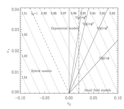
Figure 4: The various models discussed in this article represented in the plan $(\epsilon_{1},\epsilon_{2})$. The dotted lines are the lines of constant spectral index. The full lines represent the location of the large field models. The small field models are concentrated along the $\epsilon_{1}=0,\epsilon_{2}>0$ axis whereas the exponential models are along the $\epsilon_{2}=0$ line. Hybrid models have $n_{{}_{\mathrm{S}}}>1$ and $\epsilon_{2}<0$.

The results are summarized in Fig. 4 where the plan $(\epsilon_{1},\epsilon_{2})$ is represented.

IV.6 Comparison with the WMAP data

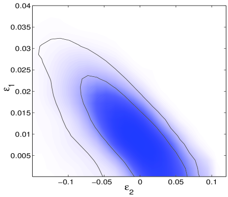
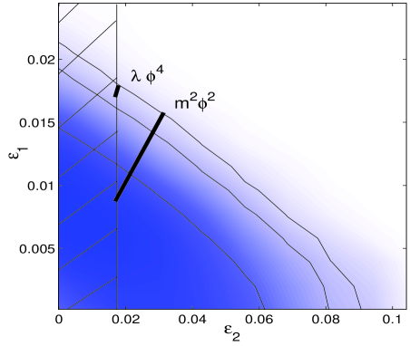
Figure 5: Left panel: allowed region in the plan $(\epsilon_{1},\epsilon_{2})$ coming from the recently released WMAP data as analyzed in Ref. LL . Right panel: zoom of the left panel. The model $V(\phi_{{}_{0}})\propto\phi_{{}_{0}}^{4}$ is now under big observational pressure. These two figures are from Ref. LL .

The aim of this section is to illustrate the fact that the high-accuracy data that are now at our disposal are now starting to discriminate among the various models of inflation presented in the last sections. The constraints coming from the most recently released CMB data, i.e. the WMAP data wmap , are represented in Fig. 5 following the analysis performed in Ref. LL . Very roughly speaking, we have the constraints $\epsilon_{1}\leq 0.05$ and $|\epsilon_{2}|\leq 0.1$.

As is clear from the previous analysis, except for a few models (like, for instance, the quadratic small field model or the exponential potential), the determination of the slow-roll parameters requires the calculation of $N_{*}$ which in turns demands the knowledge of the whole history of the universe. Unfortunately all the details of this history are not known and hence there exits important uncertainties with regards to the precise value of $N_{*}$ in a particular model. This question has been recently re-analyzed in Ref. LL2 .

Here, we just consider some examples to illustrate that, nevertheless, there exists now stringent constraints on the models. For instance, for the quadratic small field model, $|\epsilon_{2}|\lesssim 0.1$ implies that $\mu/m_{{}_{\mathrm{Pl}}}\gtrsim 1$ which is problematic for this model. For the exponential model, $\epsilon_{1}\lesssim 0.05$ means that $\beta\lesssim-2.053$. In terms of the equation of state parameter, this means (since one must have $\beta\leq-2$), $-1\lesssim p/\rho\lesssim-0.966$ during inflation. More importantly, the chaotic models are now severely constrained. In Refs. LL ; LL2 , it has been shown that there is a limit on $N_{*}$ which implies that $\epsilon_{2}\gtrsim 0.02$ (for chaotic models). This means that the models $V\propto\phi_{{}_{0}}^{n}$, with $n\geq 4$ are now under big pressure, as summarized in the right panel in Fig. 5. Other important conclusions can be obtained (in particular on the energy scale of inflation) and we refer the reader to Ref. LL for more details.

V Open issues for inflation and conclusions

Despite its impressive successes, inflation has problems. For instance, it would be clearly desirable to embed slow-roll inflation into a realistic model of particle physics at high energies (SUSY, SUGRA, string theory etc …). Unfortunately, no obvious candidate has yet emerged (for a complete discussion of the model building problem, see Ref. LR ).

Yet another open issue is the so-called trans-Planckian problem of inflation MB . This is the fact that, at the beginning of inflation, the scales of astrophysical relevance today were smaller than the Planck length, i.e. where in a regime where quantum field theory is expected to break down. Since the standard calculation of the power spectrum is based on quantum field theory, this questions the validity of its derivation. It is not easy to predict to which modifications this could give rise since quantum gravity is not known. Fortunately, one can show that “reasonable” modifications of high-energy physics can leave an imprint on the observables MR like the CMBR multipole moments. Therefore, there is a hope to constrain the new physics with (future) high accuracy cosmological observations. This would be a concrete realization of the idea that cosmology can help us to understand high energy physics.

Acknowledgments

I would like to thank P. Peter and D. Schwarz for useful discussions and careful reading of the manuscript. I am especially indebted to S. Leach and A. Liddle for the authorization to use the figures of their article LL .

References

- (1) A. Guth, Phys. Rev. D 23, 347 (1981); A. Linde, Phys. Lett. B 108, 389 (1982); A. Albrecht and P. J. Steinhardt, Phys. Rev. Lett. 48, 1220 (1982); A. Linde, Phys. Lett. B 129, 177 (1983).
- (2) V. Mukhanov and G. Chibisov, JETP Lett. 33, 532 (1981); Sov. Phys. JETP 56, 258 (1982).
- (3) S. Hawking, Phys. Lett. 115B, 295 (1982); A. Starobinsky, Phys. Lett. 117B, 175 (1982); A. Guth and S.Y. Pi, Phys. Rev. Lett. 49, 1110 (1982); J. M. Bardeen, P. J. Steinhardt, and M. S. Turner, Phys. Rev. D 28, 679 (1983).
- (4) S. Leach, A. R. Liddle, J. Martin and D. J. Schwarz, Phys. Rev. D 66, 023515 (2002), eprint astro-ph/0202094.
- (5) C. L. Bennet at al., Astrophys. J. Suppl. 148, 1 (2003), eprint astro-ph/0302207.
- (6) S. Dodelson, eprint hep-ph/0309057.
- (7) G. F. Smooth, et al., Astrophys. J. 396, L1 (1992).
- (8) G. F. R. Ellis and W. Stoeger, Class. Quant. Grav. 5, 207 (1988).
- (9) E. D. Stewart and D. H. Lyth, Phys. Lett. 302B, 171 (1993).
- (10) D. J. Schwarz, C. A. Terrero-Escalante and A. A. Garcia, Phys. Lett B517, 243 (2001), eprint astro-ph/0106020.
- (11) V. F. Mukhanov, H. A. Feldman, and R. H. Brandenberger, Phys. Rep. 215, 203 (1992).
- (12) J. A. Bardeen, Phys. Rev. D 22, 1882 (1980).
- (13) D. H. Lyth, Phys. Rev. D 31, 1792 (1985).
- (14) J. Martin and D. J. Schwarz, Phys. Rev. D 57, 3302 (1998).
- (15) L. P. Grishchuk, Zh. Eksp. Teor. Fiz 67, 825 (1974).
- (16) J. Martin and P. Peter, Phys. Rev. D 68, 103517 (2003), eprint hep-th/0307077; J. Martin and P. Peter, to appear in Physical Review Letters, eprint astro-ph/0312488.
- (17) J. Martin and D. J. Schwarz, Phys. Rev. D 67, 083512 (2003).
- (18) H. A. Kramers, Zeit. f. Physik 39, 836 (1926).
- (19) L. A. Young and G. E. Uhlenbeck, Phys. Rev. 36, 1158 (1930).
- (20) R. E. Langer, Phys. Rev. 51, 669 (1937).
- (21) J. Martin and D. J. Schwarz, Phys. Rev. D 62, 103520 (2000), eprint astro-ph/9911225; J. Martin, A. Riazuelo and D. J. Schwarz, Astrophys. J. 543, L99 (2000), eprint astro-ph/0006392.
- (22) W. H. Kinney and K. T. Mahanthappa, Phys. Rev. D 53, 5455 (1996), eprint hep-ph/9512241; S. Dodelson, W. H. Kinney and E. W. Kolb, Phys. Rev. D 56, 3207 (1997), eprint astro-ph/9702166.
- (23) S. Leach and A. Liddle, eprint astro-ph/0306305.
- (24) A. Liddle and S. Leach, Phys. Rev. D 68, 103503 (2003), eprint astro-ph/0305263.
- (25) D. Lyth and A. Riotto, Phys. Rept. 314, 1 (1999), eprint hep-ph/9807278.
- (26) J. Martin and R. H. Brandenberger, Phys. Rev. D 63, 123501 (2001), eprint hep-th/0005209; R. H. Brandenberger and J. Martin, Mod. Phys. Lett. A16, 999 (2001), eprint astro-ph/0005533.
- (27) J. Martin and C. Ringeval, eprint astro-ph/0310382.