Observations and Theoretical Implications of the Large Separation Lensed Quasar SDSS J1004+4112

Abstract

We study the recently discovered gravitational lens SDSS J1004+4112, the first quasar lensed by a cluster of galaxies. It consists of four images with a maximum separation of $14\farcs 62$. The system was selected from the photometric data of the Sloan Digital Sky Survey (SDSS), and has been confirmed as a lensed quasar at $z=1.734$ on the basis of deep imaging and spectroscopic follow-up observations. We present color-magnitude relations for galaxies near the lens plus spectroscopy of three central cluster members, which unambiguously confirm that a cluster at $z=0.68$ is responsible for the large image separation. We find a wide range of lens models consistent with the data, and despite considerable diversity they suggest four general conclusions: (1) the brightest cluster galaxy and the center of the cluster potential well appear to be offset by several kiloparsecs; (2) the cluster mass distribution must be elongated in the North–South direction, which is consistent with the observed distribution of cluster galaxies; (3) the inference of a large tidal shear ($\sim$0.2) suggests significant substructure in the cluster; and (4) enormous uncertainty in the predicted time delays between the images means that measuring the delays would greatly improve constraints on the models. We also compute the probability of such large separation lensing in the SDSS quasar sample, on the basis of the Cold Dark Matter model. The lack of large separation lenses in previous surveys and the discovery of one in SDSS together imply a mass fluctuation normalization $\sigma_{8}=1.0^{+0.4}_{-0.2}$ (95% confidence), if cluster dark matter halos have an inner density profile $\rho\propto r^{-1.5}$. Shallower profiles would require higher values of $\sigma_{8}$. Although the statistical conclusion might be somewhat dependent on the degree of the complexity of the lens potential, the discovery of SDSS J1004+4112 is consistent with the predictions of the abundance of cluster-scale halos in the Cold Dark Matter scenario.

1 Introduction

Since the discovery of the first gravitationally lensed quasar Q0957+561 (Walsh, Carswell, & Weymann, 1979), about 80 strong lens systems have been found so far. All of the lensed quasars have image separations smaller than $7^{\prime\prime}$, and they are lensed by massive galaxies (sometimes with small boosts from surrounding groups or clusters of galaxies). The probability that distant quasars are lensed by intervening galaxies was originally estimated by Turner, Ostriker, & Gott (1984) to be 0.1%–1%, assuming that galaxies can be modeled as singular isothermal spheres (SIS). This prediction has been verified by several optical and radio lens surveys, such as the Hubble Space Telescope (HST) Snapshot Survey (Bahcall et al., 1992), the Jodrell Bank/Very Large Array Astrometric Survey (JVAS; Patnaik et al., 1992), and the Cosmic Lens All Sky Survey (CLASS; Myers et al., 1995). The lensing probability is sensitive to the volume of the universe, so it can be used to place interesting constraints on the cosmological constant $\Omega_{\Lambda}$ (Turner, 1990; Fukugita, Futamase, & Kasai, 1990; Kochanek, 1996; Chiba & Yoshii, 1999; Chae et al., 2002, but see Keeton 2002).

In contrast, lenses with larger image separations should probe a different deflector population: massive dark matter halos that host groups and clusters of galaxies. Such lenses therefore offer valuable and complementary information on structure formation in the universe, including tests of the Cold Dark Matter (CDM) paradigm (Narayan & White, 1988; Cen et al., 1994; Wambsganss et al., 1995; Kochanek, 1995; Flores & Primack, 1996; Nakamura & Suto, 1997). So far the observed lack of large separation lensed quasars has been used to infer that, unlike galaxies, cluster-scale halos cannot be modeled as singular isothermal spheres (Keeton, 1998; Porciani & Madau, 2000; Kochanek & White, 2001; Keeton, 2001a; Sarbu, Rusin, & Ma, 2001; Li & Ostriker, 2002, 2003; Oguri, 2002; Ma, 2003). The difference can probably be ascribed to baryonic processes: baryonic infall and cooling have significantly modified the total mass distribution in galaxies but not in clusters (Rees & Ostriker, 1977; Blumenthal et al., 1986; Kochanek & White, 2001). As a result, large separation lenses may constrain the density profiles of dark matter halos of cluster more directly than small separation lenses (Maoz et al., 1997; Keeton & Madau, 2001; Wyithe, Turner, & Spergel, 2001; Takahashi & Chiba, 2001; Li & Ostriker, 2002; Oguri et al., 2002; Oguri, 2003; Huterer & Ma, 2004; Kuhlen, Keeton, & Madau, 2004). Alternatively, large separation lensed quasars may be used to place limits on the abundance of massive halos if the density profiles are specified (Narayan & White, 1988; Wambsganss et al., 1995; Kochanek, 1995; Nakamura & Suto, 1997; Mortlock & Webster, 2000; Oguri, 2003; Lopes & Miller, 2004). Better yet, the full distribution of lens image separations may provide a systematic diagnostic of baryonic effects from small to large scales in the CDM scenario.

The fact that clusters have less concentrated mass distributions than galaxies implies that large separation lensed quasars should be less abundant than small separation lensed quasars by one or two orders of magnitude. This explains why past surveys have failed to unambiguously identify large separation lensed quasars (Kochanek, Falco, & Schild, 1995; Phillips, Browne, & Wilkinson, 2001a; Zhdanov & Surdej, 2001; Ofek et al., 2001, 2002). For instance, CLASS found 22 small separation lenses but no large separation lenses among $\sim$15000 radio sources (Phillips et al., 2001b). Although several large separation lensed quasar candidates have been found (e.g., Mortlock, Webster, & Francis, 1999), they are thought to be physical (unlensed) pairs on the basis of individual observations (e.g., Green et al., 2002) or statistical arguments (Kochanek, Falco, & Muñoz, 1999; Rusin, 2002). Recently Miller et al. (2004) found 6 candidate lens systems with image separations $\theta>30^{\prime\prime}$ among $\sim$20000 quasars in the Two-degree Field (2dF) quasar sample. Given the lack of high-resolution spectra and deep imaging for the systems, however, it seems premature to conclude that they are true lens systems. We note that because the expected number of lenses with such large image separations in the 2dF sample is much less than unity (Oguri, 2003), these systems would present a severe challenge to standard models if confirmed as lenses.

To find a first unambiguous large separation lensed quasar, we started a project to search for large separation lenses in the quasar sample of the Sloan Digital Sky Survey (SDSS; York et al., 2000). This project complements ongoing searches for small separation lenses in SDSS (e.g., Pindor et al., 2003; Inada et al., 2003a). The SDSS has completed less than half of its planned observations, but already it contains more than 30000 quasars and is superior to previous large separation lens surveys in several ways. The full SDSS sample will comprise $\sim$100000 quasars, so we ultimately expect to find several large separation lensed quasars (Keeton & Madau, 2001; Takahashi & Chiba, 2001; Li & Ostriker, 2002; Kuhlen et al., 2004). One of the most important advantages of the SDSS in searching for large separation lensed quasars is that imaging in five broad optical bands allows us to select lens candidates quite efficiently.

Recently we reported the discovery of the large separation lensed quasar SDSS J1004+4112 at $z=1.73$ (Inada et al., 2003b) in the SDSS. The quasar itself turned out to be previously identified in the ROSAT All Sky Survey (Cao, Wei, & Hu, 1999) and the Two-Micron All-Sky Survey (Barkhouse & Hall, 2001), but was not recognized as a lensed system. Inada et al. (2003b) showed that SDSS J1004+4112 consists of four quasar images with the same redshift from the Keck spectroscopy. The colors of galaxies found by Subaru imaging follow-up observations indicated the presence of a cluster of galaxies at $z=0.68$. Moreover, the configuration of the four images was successfully reproduced by a simple lens model based on a singular isothermal ellipsoid mass distribution. All these results strongly implied that SDSS J1004+4112 is the first quasar lens system due to a massive cluster-scale object. In this paper, we describe photometric and spectroscopic follow-up observations of SDSS J1004+4112 in detail. We discuss the spectra of lensed quasar components, including puzzling differences between emission lines seen in the different images. We analyze deep multicolor imaging data to show the existence of a lensing cluster more robustly. We also present detailed mass modeling of the lens, and discuss the implications of this system for the statistics of large separation lenses.

The paper is organized as follows. Section 2 describes the method used to identify large separation lens candidates in the SDSS data. The results of follow-up observations are summarized in §3. In §4 we perform mass modeling of SDSS J1004+4112, and in §5 we consider the statistical implications of the discovery of SDSS J1004+4112. We summarize our results and conclusions in §6. Throughout this paper, we assume the popular “concordance” cosmology with $\Omega_{M}=0.27$, $\Omega_{\Lambda}=0.73$, and $H_{0}=70$ km s^-1 Mpc^-1 (e.g., Spergel et al., 2003).

2 Candidate Selection from the SDSS Object Catalog

The SDSS is a survey to image a quarter of the Celestial Sphere at high Galactic latitude and to measure spectra of galaxies and quasars found in the imaging data (Blanton et al., 2003). The dedicated 2.5-meter telescope at Apache Point Observatory (APO) is equipped with a multi-CCD camera (Gunn et al., 1998) with five broad bands centered at $3561$, $4676$, $6176$, $7494$, and $8873$ Å (Fukugita et al., 1996). The imaging data are automatically reduced by a photometric pipeline (Lupton et al., 2001). The astrometric positions are accurate to about $0\farcs 1$ for sources brighter than $r=20.5$ (Pier et al., 2003). The photometric errors are typically less than 0.03 magnitude (Hogg et al., 2001; Smith et al., 2002). The SDSS quasar selection algorithm is presented in Richards et al. (2002). The SDSS spectrographs are used to obtain spectra, covering $3800$–$9200$ Å at a resolution of $1800$–$2100$, for the quasar candidates. The public data releases of the SDSS are described in Stoughton et al. (2002) and Abazajian et al. (2003).

Large separation lens candidates can be identified from the SDSS data as follows. First, we select objects that were initially identified as quasars by the spectroscopic pipeline. Specifically, among SDSS spectroscopic targets we select all objects that have spectral classification of SPEC_QSO or SPEC_HIZ_QSO with confidence z_conf larger than $0.9$ (see Stoughton et al., 2002, for details of the SDSS spectral codes). Next we check the colors of nearby unresolved sources to see if any of those sources could be an additional quasar image, restricting the lens search to separations $\theta<60^{\prime\prime}$. We define a large separation lens by $\theta>7^{\prime\prime}$ so that it exceeds the largest image separation lenses found so far: Q0957+561 with $\theta=6\farcs 26$ (Walsh et al., 1979) and RX J0921+4529 with $\theta=6\farcs 97$ (Muñoz et al., 2001), both of which are produced by galaxies in small clusters. We regard the stellar object as a candidate companion image if the following color conditions are satisfied:

$$\left|\Delta(j-k)\right| < 3\sigma_{\Delta(j-k)}$$ (1)

$$= 3\sqrt{\left(\sigma_{j,{\rm err}}^{2}+\sigma_{k,{\rm err}}^{2}\right)_{\rm quasar}+\left(\sigma_{j,{\rm err}}^{2}+\sigma_{k,{\rm err}}^{2}\right)_{\rm stellar}},$$

$$\left|\Delta(j-k)\right|<0.1,$$ (2)

$$\left|\Delta i^{*}\right|<2.5,$$ (3)

where $\{j,k\}=\{u^{*},g^{*}\}$, $\{g^{*},r^{*}\}$, $\{r^{*},i^{*}\}$, and $\{i^{*},z^{*}\}$, and $\Delta$ denotes the difference between the spectroscopically identified quasar and the nearby stellar object. Note that this selection criterion is tentative; we still do not know much about large separation lenses, so selection criteria may evolve as we learn more.

Redshift distribution of quasars identified by the spectroscopic pipeline in the SDSS. Dashed vertical lines show the redshift cut $0.6<z<2.3$ used for the statistical analysis.

Our full sample contains 44269 quasars with the redshift distribution shown in Figure 2. For the lens search we select the subset of 29811 quasars with $0.6<z<2.3$, making the redshift cuts for four reasons: (1) at $z<0.6$ quasars are often extended, which can complicated both lens searches and also lens statistics analyses; (2) at $z<0.6$ the sample is contaminated by narrow emission line galaxies; (3) at $z>2.3$ we may miss a number of quasar candidates because of large color errors; and (4) lens statistics calculations for high redshift quasars are not very reliable because of uncertainties in the quasar luminosity function (Wyithe & Loeb, 2002a, b). Lens surveys of high-redshift quasars are of course very interesting for insights into the abundance and formation of distant quasars; a search for lenses among high-redshift SDSS quasars is the subject of a separate analysis by Richards et al. (2004).

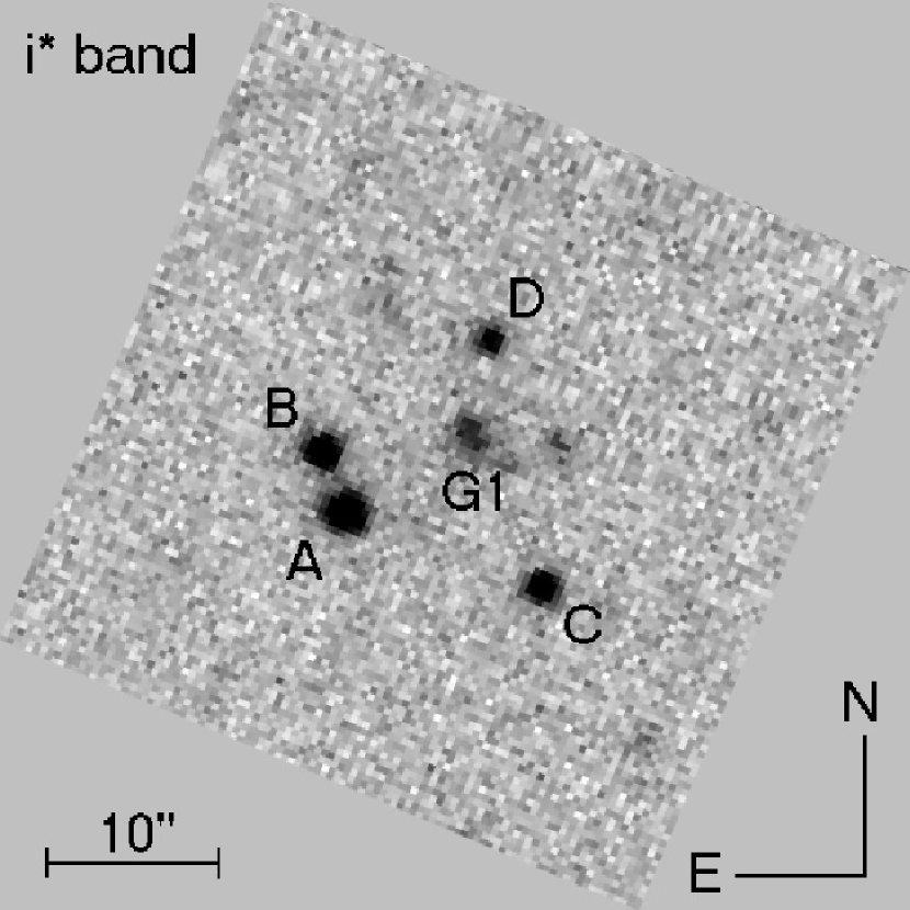
Figure 1: SDSS $i^{*}$-band image of SDSS J1004+4112. Components A, B, C, and D are lensed images while component G1 is the brightest galaxy in the lensing cluster.

SDSS J1004+4112 was first selected as a lens candidate based on a pair of components, A and B (see Figure 1), where B is the SDSS spectroscopic target. Components C and D were identified by visual inspection and found to have colors similar to those of A and B (even though they do not match the above color criteria). Table 1 summarizes the photometry for the four components, and Table 2 gives the astrometry for the four components as well as the galaxy G1 seen in Figure 1. The reason that components C and D have somewhat different colors from B is still unclear, but it must be understood in order to discuss the completeness of the lens survey. The difference might be ascribed to differential absorption or extinction by intervening material (Falco et al., 1999), or to variability in the source on time scales smaller than the time delays between the images (e.g., de Vries, Becker, & White, 2003), both of which are effects that become more important as the image separation grows.

3 Data Analysis

3.1 Spectroscopic Follow-up Observations

3.1.1 Quasar Images

Since only component B has a spectrum from SDSS, we obtained spectra of the other components to investigate the lensing hypothesis. The first spectroscopic follow-up observations were done on 2003 May 2 and 5 with the Double Imaging Spectrograph of the Astrophysical Research Consortium (ARC) 3.5-m telescope at APO. All four components have a prominent C IV emission line ($1549.06$ Å) at $\lambda_{\rm obs}\sim 4230$ Å, indicating that they are quasars with very similar redshifts. Spectra with higher resolution and longer wavelength range were taken on 2003 May 30 with the Low-Resolution Imaging Spectrometer (LRIS; Oke et al., 1995) of the Keck I telescope at the W. M. Keck Observatory on Mauna Kea, Hawaii, USA. The blue grism is 400 line mm^-1, blazed at $3400$ Å, $1.09$ Å pixel^-1, covering $3000$ Å to $5000$ Å. The red grating is 300 line mm^-1, blazed at $5000$ Å, $1.09$ Å pixel^-1, covering $5000$ Å to the red limit of the detector. The spectra were obtained with 900 sec exposures and a $1^{\prime\prime}$ slit in $0\farcs 9$ seeing. The data were reduced in a standard way using IRAF. The Keck/LRIS spectra are shown in Figure 2. All four components show emission lines of Ly$\alpha$, Si IV, C IV, C III], and Mg II. They have nearly identical redshifts of $z=1.734$, with velocity differences less than $50\,{\rm km\,s^{-1}}$ (see Table 1). The flux ratios between the images (see Figure 2) are almost constant over the wavelength range 3000–8000 Å, indicating that these are actual lensed images. From the spectra, we conclude that the color differences found in the SDSS images are mainly caused by differences in the emission lines (discussed below) and by slightly different continuum slopes.

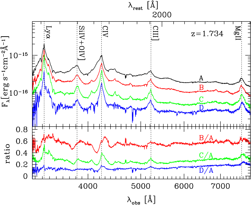
Figure 2: Spectra (top) and flux ratios (bottom) of SDSS J1004+4112 components A, B, C, and D taken with LRIS on Keck I. In the upper panel, we can confirm that all components have Ly$\alpha$, Si IV, C IV, C III] , and Mg II emission lines at $z=1.734$. The flux ratios shown in the lower panel are almost constant for a wide range of wavelength. Several absorption lines are also seen in the spectra (see text for details).

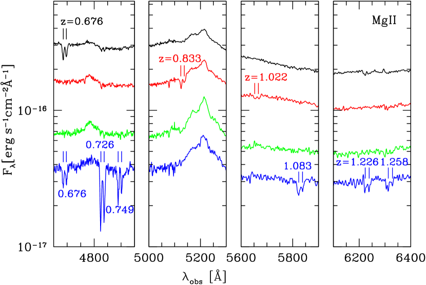
Figure 3: The Mg II doublet absorption lines (rest frame wavelengths of $2795.5$ Å and $2802.7$ Å, rest frame equivalent width $W_{\rm r}\gtrsim 0.5$ Å) of SDSS J1004+4112 components A, B, C, and D at various wavelengths. The absorption lines are indicated by vertical lines.

Several absorption line systems are seen in the spectra. Components A and D have intervening Mg II/Fe II absorption systems at $z=0.676$; this redshift is similar to that of the foreground galaxies (§3.1.2), suggesting that this absorption system is associated with the lensing galaxies. Component D has additional Mg II absorption systems at $z=0.726$, $0.749$, $1.083$, $1.226$, and $1.258$. Figure 3 identifies the various Mg II absorbers. We also note that all four components have C IV absorption lines just blueward of C IV emission lines (see Figure 3.1.1). The velocity difference between the emission and absorption lines is $\sim\!500\,{\rm km\,s^{-1}}$, so the absorption system is likely to be associated with the quasar. The fact that all four components have C IV absorption lines offers further evidence that SDSS J1004+4112 is indeed a gravitational lens.

The C IV lines of SDSS J1004+4112 components A, B, C, and D taken with LRIS. The associated C IV doublet absorption lines (rest frame wavelengths $1548.2$ Å and $1550.8$ Å, denoted by dotted lines) are seen in all four components.

Figure 3.1.1 shows notable differences in the C IV emission line profiles in the different components. One possible explanation is the time delay between the lensed images; at any given observed epoch, the images represent different epochs in the source frame. However, the fact that the C IV emission lines in components A and B differ seems to rule out the time delay explanation: the expected delay (see §4.2.2) is shorter than the month or year time scale on which C IV emission lines typically vary (e.g., Vanden Berk et al., 2004). Other possible explanations include differences between the viewing angles probed by the images, microlensing amplification of part of the quasar emission region, significant errors in the predicted time delay between A and B, or just that the quasar is extremely unusual. Understanding the puzzling line profile differences will require further observations, preferably including measurement of the time delays and spectroscopic monitoring to identify any variability in the C IV lines.

3.1.2 Galaxies

Spectrum of the galaxy G1 taken with LRIS on Keck I. The break, Ca II H&K absorption lines, and Mg absorption line are consistent with redshift $z=0.680$ ($z=0.6799\pm 0.0001$ from the Ca II H line). The G-band also appears in the spectrum.

The spectrum of the galaxy G1, the brightest object near the center of the quasar configuration (see Figure 1), was acquired on 2003 May 30 with LRIS. The spectrum measured from a 900 sec exposure is shown in Figure 3.1.2. We confirm the break and Ca II H&K lines at $\lambda_{\rm obs}\sim 6700$ Å. The G-band also appears in the spectrum. From the Ca II H&K and Mg lines we derive the redshift of G1 as $z=0.680$.

Spectra of galaxies G2 and G3 taken with FOCAS on the Subaru 8.2-m telescope. From the absorption lines Ca II H&K, H$\delta$, and G-band, we find that the redshifts of both galaxies are $z=0.675$ ($z=0.6751\pm 0.0001$ from the H$\delta$ lines).

The spectra of two additional galaxies near G1 (see §3.2) were taken on 2003 June 20 with the Faint Object Camera and Spectrograph (FOCAS; Kashikawa et al., 2002) on the Subaru 8.2-m telescope of the National Astronomical Observatory of Japan on Mauna Kea, Hawaii, USA. We used the 300B grism together with the SY47 filter, and took optical spectra covering $4100$ Å to $10000$ Å with resolution $2.84$ Å pixel^-1. The seeing was $0\farcs 7$, and the exposure time was 1740 sec for both galaxies. The data were reduced in a standard way using IRAF. The spectra are shown in Figure 3.1.2. Both galaxies, denoted as G2 and G3, have $z=0.675$, only $\sim\!700\,{\rm km\,s^{-1}}$ from the redshift of G1.

3.2 Imaging Follow-up Observations

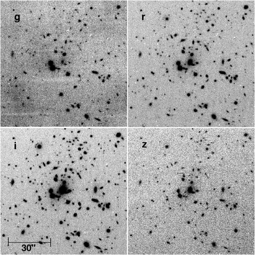
Figure 4: Deep $griz$ images taken with Suprime-Cam on the Subaru 8.2-m telescope. The exposure details are summarized in Table 3.

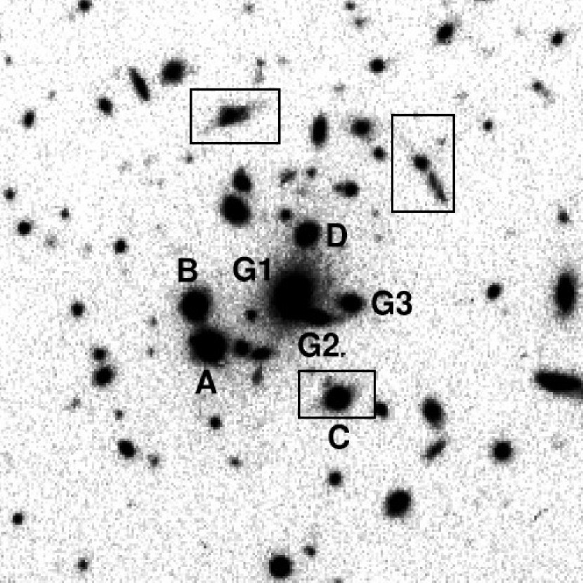
Figure 5: The central region of the Suprime-Cam $i$-band image. The galaxies with measured redshifts (G1 from LRIS and G2 and G3 from FOCAS) as well as the four lensed images are labeled. The possible lensed arclets are marked with rectangles.

3.2.1 Observations

A deep $r$-band image of SDSS J1004+4112 was taken on 2003 May 5 with the Seaver Prototype Imaging camera of the ARC 3.5-m telescope at APO. The image shows rich structure, with many galaxies between and around the quasar components suggesting a possible galaxy cluster in the field. For a further check, we obtained deeper multi-color ($griz$) images on 2003 May 28 with the Subaru Prime Focus Camera (Suprime-Cam; Miyazaki et al., 2002) on the Subaru 8.2-m telescope. The exposure times and limiting magnitudes of the Suprime-Cam images are given in Table 3. Suprime-Cam has a pixel scale of $0\farcs 2\,{\rm pixel^{-1}}$, and the seeing was $0\farcs 5$–$0\farcs 6$. The frames were reduced (bias-subtracted and flat-field corrected) in a standard way. The resulting images are shown in Figure 4. It is clear that there are many red galaxies around the four images. Moreover, we find three possible lensed arclets (distorted images of galaxies behind the cluster), which are shown in more detail in Figure 5. The fact that the arclets are relatively blue compared with the brighter galaxies in the field (see Figure 2 in Inada et al., 2003b) suggests that the arclets may be images of distant galaxies (e.g., Colley, Tyson, & Turner, 1996). Confirming that they are lensed images will require higher resolution images and measurements of the arclets’ redshifts. If the hypothesis is confirmed, the arclets will provide important additional constraints on the lens mass distribution.

3.2.2 Colors of Nearby Galaxies

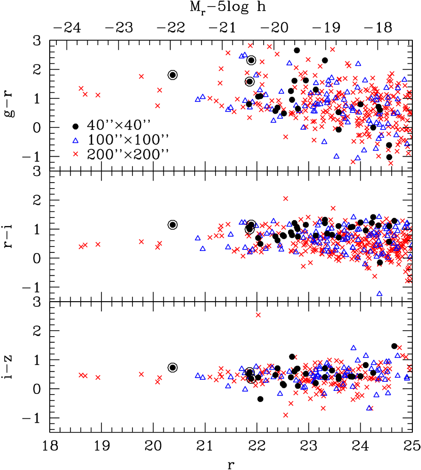
Figure 6: Color-magnitude diagrams for the SDSS J1004+4112 field taken with Suprime-Cam. We divide the galaxies into three categories according to their positions: filled circles denote galaxies inside a $40^{\prime\prime}\times 40^{\prime\prime}$ box centered on G1, open triangles denote galaxies inside a $100^{\prime\prime}\times 100^{\prime\prime}$ box, and crosses denote galaxies inside a $200^{\prime\prime}\times 200^{\prime\prime}$ box. These box sizes correspond to $0.2h^{-1}\,{\rm Mpc}\times 0.2h^{-1}{\rm Mpc}$, $0.5h^{-1}{\rm Mpc}\times 0.5h^{-1}{\rm Mpc}$, and $1.0h^{-1}{\rm Mpc}\times 1.0h^{-1}{\rm Mpc}$ at $z=0.68$, respectively. Three spectroscopically confirmed member galaxies are marked with open circles. The corresponding $r$-band absolute magnitudes at $z=0.68$ (without K-correction) are given at the top of the frame.

The colors of galaxies in the vicinity of SDSS J1004+4112 can help us search for the signature of a cluster. The central regions of clusters are dominated by early-type galaxies (e.g., Dressler, 1980) that show tight correlations among their photometric properties (Bower, Lucey, & Ellis, 1992). These correlations make it possible to search for clusters using color-magnitude and/or color-color diagrams (Dressler & Gunn, 1992; Gladders & Yee, 2000; Goto et al., 2002).

We measure the colors of galaxies using the deep Suprime-Cam $griz$ images. Object identifications are performed using the Source Extractor algorithm (SExtractor; Bertin & Arnouts, 1996); we identify objects with SExtractor parameter CLASS_STAR smaller than 0.6 in the $i$ band image as galaxies. Note that this star/galaxy separation criterion is successful only for objects with $i\lesssim 24$. The magnitudes in the images are calibrated using nearby stars whose magnitudes are taken from the SDSS photometric data.

Since the red galaxies in clusters are dominant in the central regions, and the center of the cluster is thought to be near G1, we divide the galaxies in the field into three categories: galaxies inside a $40^{\prime\prime}\times 40^{\prime\prime}$ (corresponding to $0.2h^{-1}{\rm Mpc}\times 0.2h^{-1}{\rm Mpc}$ at $z=0.68$) box centered on G1; galaxies inside a $100^{\prime\prime}\times 100^{\prime\prime}$ ($0.5h^{-1}{\rm Mpc}\times 0.5h^{-1}{\rm Mpc}$) box (except for those in the first category); and galaxies inside a $200^{\prime\prime}\times 200^{\prime\prime}$ ($1.0h^{-1}{\rm Mpc}\times 1.0h^{-1}{\rm Mpc}$) box (except for those in the first two categories). Figure 6 shows color-magnitude diagrams for the three categories. It is clear that the color-magnitude relations, particularly $r-i$ and $i-z$, show tight correlations for galaxies inside the $40^{\prime\prime}\times 40^{\prime\prime}$ box. Ridge lines at $r-i\sim 1.1$ and $i-z\sim 0.5$ strongly suggest a cluster of galaxies at $z\sim 0.6$ (Goto et al., 2002). The result is consistent with the Keck and Subaru spectroscopic results showing that the redshifts of galaxies G1, G2, and G3 are all $z\sim 0.68$.

We identify cluster members by their location in color-color space (Dressler & Gunn, 1992; Goto et al., 2002). We show $g-r-i$ and $r-i-z$ color-color diagrams in Figures 3.2.2 and 3.2.2, respectively. We restrict the plots to galaxies brighter than $i=24$ because of the limitation of the star/galaxy separation. We make color-color cuts based on the colors expected of elliptical galaxies (Fukugita, Shimasaku, & Ichikawa, 1995): $g-r>1.5$, $r-i>0.7$, and $i-z>0.2$ for elliptical galaxies at $z\gtrsim 0.5$. The galaxy distributions with and without the color cuts are shown in Figure 7. The galaxies that survive the color cuts are concentrated around G1, so we conclude that they are candidate members of a cluster of galaxies at $z=0.68$ whose center is near G1. We note that the distribution of candidate cluster members is not spherical and appears to be elongated North–South.

The $g-r-i$ color-color diagram of galaxies brighter than $i=24$. Symbols are the same as in Figure 6. Dotted lines indicate color cuts to find cluster members.

Similar to Figure 3.2.2, but for $r-i-z$.

Figure 7: Distributions of galaxies brighter than $i=24$ with (right) and without (left) the color cut. The origin $(0,0)$ is set to the position of the central galaxy G1. Filled squares denote the four lensed images.

4 Mass Modeling

4.1 One-component Models

To search for mass models that can explain the image configuration of SDSS J1004+4112, we use standard lens modeling techniques as implemented in the software of Keeton (2001b). The main constraints come from the image positions. We also use the flux ratios as constraints, although we broaden the errorbars to 20% to account for possible systematic effects due to source variability and time delays, micro- or milli-lensing, or differential extinction (See Table 4 for the full set of constraint data). In particular, the different colors of the images and the different absorption features seen in Figure 2 suggest that differential extinction may be a significant effect. In this section we do not use the position of the main galaxy as a constraint, because we want to understand what constraints can be placed on the center of the lens potential from the lens data alone.

We first consider the simplest possible models for a 4-image lens: an isothermal lens galaxy with a quadrapole produced either by ellipticity in the galaxy or by an external shear. A spherical isothermal lens galaxy has surface mass density

$$\kappa(r)=\frac{\Sigma(r)}{\Sigma_{\rm crit}}=\frac{r_{\rm ein}}{2r}\ ,$$ (4)

where $r_{\rm ein}$ is the Einstein radius of the lens, and $\Sigma_{\rm crit}=(c^{2}/4\pi G)(D_{\rm OS}/D_{\rm OL}D_{\rm LS})$ is the critical surface mass density for lensing, with $D_{\rm OL}$, $D_{\rm OS}$, and $D_{\rm LS}$ being angular diameter distances from the observer to the lens, from the observer to the source, and from the lens to the source, respectively. The Einstein radius is related to the velocity dispersion $\sigma$ of the galaxy by

$$r_{\rm ein}=4\pi\,\left(\frac{\sigma}{c}\right)^{2}\,\frac{D_{\rm LS}}{D_{\rm OS}}\ .$$ (5)

For an elliptical model we replace $r$ with $r[1+((1-q^{2})/(1+q^{2}))\cos 2(\theta-\theta_{e})]^{1/2}$ in the surface density, where $q$ and $\theta_{e}$ are the axis ratio and position angle of the ellipse.

Simple models using either pure ellipticity or pure shear fail miserably, yielding $\chi^{2}$ values no better than $2\times 10^{4}$ for $N_{\rm dof}=4$ degrees of freedom. This failure is not surprising: most 4-image lenses require both ellipticity and external shear (e.g., Keeton, Kochanek, & Seljak, 1997), and such a situation is likely in SDSS J1004+4112 since the main galaxy is observed to be elongated and the surrounding cluster surely contributes a shear.

Figure 8: Critical curve (left) and caustic (right) for the best-fit SIE+shear lens model of SDSS J1004+4112. In the left panel, the filled circles mark the image positions, the open circle indicates the observed position of the brightest cluster galaxy G1, and the cross marks the best-fit deflector position. In the right panel the filled circle marks the inferred source position.

We therefore try models consisting of a singular isothermal ellipsoid (SIE) plus an external shear $\gamma$. Even though such models are still comparatively simple, they can fit the data very well with a best-fit value of $\chi^{2}=0.33$ for $N_{\rm dof}=2$. The best-fit model has an Einstein radius $r_{\rm ein}=6\farcs 9=35\,h^{-1}$ kpc corresponding to a velocity dispersion of 700 km s^-1, an ellipticity $e=0.50$ at position angle $\theta_{e}=21\fdg 4$, and an external shear $\gamma=0.25$ at position angle $\theta_{\gamma}=-60\fdg 9$. Among other known lenses, such a large shear is found only in lenses lying in cluster environments (Burud et al., 1998; Barkana et al., 1999). Figure 8 shows the critical curves and caustics for the best-fit model. The inferred source position lies very close to the caustic and fairly near a cusp, implying that the total magnification is $\sim$57. Figure 9 shows the allowed ranges for the position of the deflector and the ellipticity and external shear in the model. The models indicate a small but significant offset of $1\farcs 6=7.9\,h^{-1}$ kpc between the center of the lens potential and the main galaxy, although it remains to be seen whether that offset is real or an artifact of these still simple lens models.

Figure 9: Likelihood contours drawn at 1$\sigma$, 2$\sigma$, and 3$\sigma$ for various parameter combinations in SIE+shear lens models. The left panel shows constraints on the position of the deflector; the circle marks the observed position of the main galaxy. The right panel shows contours in the ellipticity–external shear plane.

4.2 Two-component Models

Even though the simple SIE+shear model provides a good fit to the data, we believe that it is not physically plausible because the system clearly has multiple mass components and it seems unlikely that all of the mass is associated with a single $\sim$700 km s^-1 isothermal component. The next level of complication is to add a mass component representing the cluster halo. We still model the galaxy G1 explicitly, treating it as an isothermal ellipsoid constrained by its observed position. At this point we do not further complicate the model by attempting to treat the other galaxies within the lens explicitly.

4.2.1 Methods

We model the cluster component with an NFW profile which has been predicted in cosmological $N$-body simulations (Navarro, Frenk, & White, 1996, 1997):

$$\rho(r)=\frac{\rho_{\rm crit}(z)\delta_{\rm c}(z)}{\left(r/r_{\rm s}\right)\left(1+r/r_{\rm s}\right)^{2}},$$ (6)

where $r_{\rm s}$ is a scale radius, $\delta_{\rm c}$ is a characteristic overdensity (which depends on redshift), and $\rho_{\rm crit}(z)$ is the critical density of the universe. Although the NFW density profile appears to deviate from the results of more recent $N$-body simulations in the innermost region (Moore et al., 1999; Ghigna et al., 2000; Jing & Suto, 2000; Klypin et al., 2001; Fukushige & Makino, 1997, 2001, 2003; Power et al., 2003; Fukushige, Kawai, & Makino, 2004; Hayashi et al., 2004), we adopt this form for simplicity. The lensing properties of a spherical NFW halo are described by the lens potential (Bartelmann, 1996; Golse & Kneib, 2002; Meneghetti, Bartelmann, & Moscardini, 2003a)

$$\phi(r)=2\,\kappa_{\rm s}\,r_{\rm s}^{2}\left[\ln^{2}\frac{r}{2r_{\rm s}}-\mbox{arctanh}^{2}\sqrt{1-(r/r_{\rm s})^{2}}\right],$$ (7)

where the lensing strength is specified by the parameter

$$\kappa_{\rm s}=\frac{r_{\rm s}\delta_{\rm c}(z)\rho_{\rm crit}(z)}{\Sigma_{\rm crit}}.$$ (8)

Since asphericity in the cluster potential is important in modeling this system, we generalize the spherical model by adopting elliptical symmetry in the potential. Making the potential (rather than the density) elliptical makes it possible to compute the lensing properties of an NFW halo analytically (Golse & Kneib, 2002; Meneghetti et al., 2003a). We may still be over-simplifying the mass model, because the cluster profile may have been modified from the NFW form by baryonic processes such as gas cooling (Rees & Ostriker, 1977; Blumenthal et al., 1986), and the cluster may have a complex angular structure if it is not relaxed (e.g., Meneghetti et al., 2003a). To allow for the latter possibility, we still include a tidal shear in the lens model that can approximate the effects of complex structure in the outer parts of the cluster. Overall, our goal is not to model all of the complexities of the lens potential, but to make the minimal realistic model and see what we can learn.

Figure 10: Allowed parameter ranges for galaxy+cluster lens models with a cluster scale radius $r_{\rm s}=40^{\prime\prime}$. (a) The position of the cluster component. The filled circles mark the image positions, and the open circle marks the observed brightest cluster galaxy G1. (b) The ellipticity and position angle of the galaxy component. (c) The ellipticity and position angle of the cluster component. (d) The amplitude and position angle of the external shear. Small points show all models, while boxes mark models where the model galaxy is roughly aligned with the observed galaxy ($\theta_{e}=-19\fdg 9\pm 20\fdg 0$).

Even with our simplifying assumptions, we still have a complex parameter space with 11 parameters defining the lens potential: the mass, ellipticity, and position angle for the galaxy G1; the position, mass, scale radius, ellipticity, and position angle for the cluster; and the amplitude and position angle of the shear. There are also three parameters for the source (position and flux). With just 12 constraints (position and flux for each of four images), the models are under-constrained. We therefore expect that there may be a range of lens models that can fit the data. To search the parameter space and identify the range of models, we follow the technique introduced by Keeton & Winn (2003) for many-parameter lens modeling. Specifically, we pick random starting points in the parameter space and then run an optimization routine to find a (local) minimum in the $\chi^{2}$ surface. Repeating that process numerous times should reveal different minima and thereby sample the full range of models. Many of the recovered models actually lie in local minima that do not represent good fits to the data, so we only keep recovered models with $\chi^{2}<11.8$ (which represents the 3$\sigma$ limit relative to a perfect fit when examining two-dimensional slices of the allowed parameter range; see Press et al., 1992).

We make one further cut on the models. From the previous section, we know that an SIE+shear lens model can give a good fit to the data. Thus, there are acceptable two-component models where most or all of the mass is in the galaxy component and the cluster contribution is negligible. To exclude such models as physically implausible, we impose an upper limit on the velocity dispersion of the model galaxy. Specifically, we only keep models with $\sigma_{\rm gal}<400$ km s^-1, because there are essentially no galaxies in the observed universe with larger velocity dispersions, even in rich clusters (e.g., Kelson et al., 2002; Bernardi et al., 2003; Sheth et al., 2003). Formally, we impose this cut as an upper limit $r_{\rm ein}<2\farcs 25$ on the Einstein radius of the galaxy G1.

4.2.2 Results

Figure 11: Critical curves and caustics for sample galaxy+cluster lens models with a cluster scale radius $r_{\rm s}=40\arcsec$. In each panel, the left-hand side shows the critical curves in the image plane, and the right-hand side shows the caustics in the source plane on the same scale. The points in the image plane show the observed image positions, and the point in the source plane shows the inferred source position. The value of $\mu$ gives the total magnification in each model.

We first consider models where the scale radius of the cluster is fixed as $r_{\rm s}=40^{\prime\prime}$ (we shall justify this choice below). Figure 10 shows the allowed parameter ranges for acceptable models. First, panel (a) shows that the cluster component is restricted to a fairly small (but not excessively narrow) range of positions near the center of the image configuration. This is mainly a result of our upper limit on the mass of the galaxy component; there is a certain enclosed mass implied by the image separation, and if the galaxy cannot contain all of that mass then the cluster component must lie within the image configuration to make up the difference. It is interesting to note that even in these more complicated models there still seems to be a small offset between the center of the cluster component and the brightest cluster galaxy G1, although the lower limit implied by our models is just $0\farcs 71=3.6h^{-1}$kpc.

Figure 10b shows that the allowed values for the ellipticity and position angle of the galaxy G1 basically fill the parameter space, so these parameters are not constrained by the lens data. We might want to impose an external constraint, however. Analyses of other lens systems show that the lensing mass is typically aligned with the projected light distribution (Keeton, Kochanek, & Falco, 1998; Kochanek, 2002). We may therefore prefer lens models where the model galaxy is at least roughly aligned with the observed galaxy, which has a position angle of $-19\fdg 9$. To illustrate this possible selection, we show all models but highlight those where the position angle of the model galaxy is in the range $\theta_{e}=-19\fdg 9\pm 20\fdg 0$. The broad $20\arcdeg$ uncertainties prevent this constraint from being too strong.

Figure 10c shows that there are some acceptable models where the cluster potential is round, but most models have some ellipticity that is aligned roughly North–South. This is in good agreement with the distribution of member galaxies which is also aligned roughly North–South (see Figure 7). The ellipticity $e\sim 0.2$–0.4 is actually quite large, considering that this parameter describes the ellipticity of the potential, not that of the density. Figure 10d shows that all of the acceptable models require a fairly large tidal shear $\gamma\gtrsim 0.10$, and models where the galaxy is aligned with the observed galaxy have a strong shear $\gamma\gtrsim 0.23$. The shear tends to be aligned East–West. The fact that the models want both a large cluster ellipticity and a large tidal shear strongly suggest that there is complex structure in the cluster potential outside of the image configuration. It would be interesting to see whether there is any evidence for such structure in, for example, X-rays from the cluster.

Figure 11 shows critical curves and caustics for sample lens models. The critical curves are not well determined. The outer, tangential critical curve can point either northeast (panel e) or northwest (panel d), or it can have a complex shape (panel a). Sometimes there is just one inner, radial critical curve (panel e), but often there are two (panel c). The distance of the source from the caustic (and of the images from the critical curve) varies from model to model, so the total magnification can range from $\sim$50 to several hundred or even more. Finally, perhaps the most interesting qualitative result is that even the image parities are not uniquely determined. In most models (e.g., panels a–f) images A and D lie inside the critical curve and have negative parity while B and C lie outside the critical curve and have positive parity. However, in some models (e.g., panels g–h) the situation is reversed. Having ambiguous image parities is very rare in lens modeling.

So far we have only discussed models where the cluster has a scale radius $r_{\rm s}=40^{\prime\prime}$. We have also computed models with $r_{\rm s}=(10,20,30,50,60)$ arcsec and we find that all of the results are quite similar. To understand what value of the scale radius is reasonable, we must consider which (if any) of the models have physically plausible cluster parameters. Even though NFW models are formally specified by two parameters $r_{\rm s}$ and $\kappa_{\rm s}$, $N$-body simulations reveal that the two parameters are actually correlated. NFW models therefore appear to form a one-parameter family of models, although with some scatter which reflects the scatter of the concentration parameter $c_{\rm vir}=r_{\rm vir}/r_{\rm s}$ ($r_{\rm vir}$ is a virial radius of the cluster). Figure 4.2.2 shows the predicted relation between $r_{\rm s}$ and $\kappa_{\rm s}$, including the scatter. For comparison, it also shows the fitted values of $\kappa_{\rm s}$ in lens models with different scale radii. Models with $r_{\rm s}=10^{\prime\prime}$ or $20^{\prime\prime}$ require $\kappa_{\rm s}$ much larger than expected, corresponding to a halo that is too concentrated. Models with $r_{\rm s}\geq 30^{\prime\prime}$, by contrast, overlap with the predictions and thus are physically plausible. We can therefore conclude very roughly that the cluster component must have $r_{\rm s}\gtrsim 30^{\prime\prime}$ and a total virial mass $M\gtrsim 10^{14}\,h^{-1}\,M_{\odot}$.

Relation between the cluster scale radius $r_{\rm s}$ and lensing strength $\kappa_{\rm s}$. The solid line shows the predicted relation for clusters with the canonical median concentration, and the dotted lines show the 1$\sigma$ range due to the scatter in concentration (see §5.1.2). The labeled points show the value of $\log(M)$ (in units of $h^{-1}M_{\odot}$) at various points along the curve. The points show fitted values of $\kappa_{\rm s}$ for lens models with $r_{\rm s}=(10,20,30,40,50,60)$ arcsec. As in Figure 10, small points show all models, while boxes mark models where the model galaxy is roughly aligned with the observed galaxy.

Finally, we can use the models to predict the time delays between the images. The models always predict that the time delay between images C and D is the longest and the delay between A and B is the shortest. However, there is no robust prediction of the temporal ordering: most models predict that the sequence should be C–B–A–D, but a few models predict the reverse ordering D–A–B–C. This is a direct result of the ambiguity in the image parities, because the leading image is always a positive-parity image (e.g., Schneider, Ehlers, & Falco, 1992). We note, however, that all of the models where the model galaxy is roughly aligned with the observed galaxy have the C–B–A–D ordering.

Figure 4.2.2 shows the predictions for the long and short time delays. The long delay between C and D can be anything up to $\sim\!3000\,h^{-1}$ days, while the short delay between A and B can be up to $\sim\!37\,h^{-1}$ days. For the models where the galaxy is roughly aligned with the observed galaxy, the two delays are approximately proportional to each other with $\Delta t_{CD}/\Delta t_{BA}=143\pm 16$. These results have several important implications. First, the A–B time delay should be on the order of weeks or months, so it should be very feasible to measure it, provided that the source has detectable variations. Measuring the A–B delay would be very useful because it would determine the temporal ordering, and thereby robustly determine the image parities. In addition, it would allow a good estimate of the long C–D delay and indicate whether attempting to measure that delay would be worthwhile. Second, the enormous range of predicted time delays means that constraining the Hubble constant with this system (Refsdal, 1964) will be difficult because of large systematic uncertainties in the lens models. Although Koopmans et al. (2003) recently showed that it is possible to obtain useful constraints on the Hubble constant even in a complex system with two mass components, the analysis is very complex and requires extensive data including not just the image positions and all of the time delays, but also an Einstein ring image and the velocity dispersion of one of the mass components. Even if we obtain such data for SDSS J1004+4112 in the near future, it seems likely that it will be difficult to obtain reliable constraints on the Hubble constant given the complexity of the lens potential in SDSS J1004+4112. The time delays, however, would still be extremely useful, because they would determine the temporal ordering and hence the image parities, and they would provide constraints that can rule out many of the models that are currently acceptable.

Predictions for the longest ($\Delta t_{CD}$) and shortest ($\Delta t_{BA}$) time delays, where $\Delta t_{ij}>0$ means image $i$ leads image $j$, and vice versa. Results are shown for models where the cluster has scale length $r_{\rm s}=(30,40,50,60)$ arcsec. As in Figure 10, small points show all models, while boxes mark models where the model galaxy is roughly aligned with the observed galaxy.

5 Lens Statistics

In this section, we calculate the expected rate of large separation lensing in the SDSS quasar sample. The discovery of SDSS J1004+4112 allows us to move past the upper limits obtained from previous large separation lens searches, although at present the main thing we can do is test whether the detection of one large separation lens in the current sample is consistent with standard theoretical models in the CDM scenario.

5.1 Modeling Lens Probabilities

We calculate lensing probabilities using spherical models for simplicity. Although halos in CDM simulations are in fact triaxial (e.g., Jing & Suto, 2002), the spherical assumption is often adopted in lens statistics calculations because deviations from spherical symmetry mainly affect image multiplicities, not image separations or the total optical depth for lensing (e.g., Kochanek, 1996; Keeton et al., 1997; Chae, 2003). While this result has been obtained for isothermal lens potentials, checking it for more general halos is beyond the scope of this paper and is the subject of a follow-up analysis (M. Oguri et al., in prep.).

5.1.1 Lens Probabilities

Let the physical image position in the lens plane and physical source position in the source plane as $\xi$ and $\eta$, respectively. Consider the probability that a quasar at $z_{\rm S}$ with luminosity $L$ is strongly lensed. The probability of lensing with image separation larger than $\theta$ is given by

$$P^{\rm B}(>\!\theta;z_{\rm S},L) = \int_{0}^{z_{\rm S}}dz_{\rm L}\,(1+z_{\rm L})^{3}\,\frac{c\,dt}{dz_{\rm L}}$$ (9)

$$\times\int_{M_{\rm min}}^{\infty}dM\,\frac{dn}{dM}\ \sigma_{\rm lens}\ B(z_{\rm S},L)$$

where $\sigma_{\rm lens}=\pi\,\eta_{\rm r}^{2}\,D_{\rm OL}^{2}/D_{\rm OS}^{2}$ is the cross section for lensing, with $\eta_{\rm r}$ being the physical radius of the radial caustic in the source plane. The lower limit of the mass integral is the mass $M_{\rm min}$ that corresponds to the image separation $\theta$; this can be computed once the density profile of the lens object is specified. The magnification bias $B(z_{\rm S},L)$ is (Turner, 1980; Turner et al., 1984)

$$B(z_{\rm S},L)=\frac{2}{\eta_{\rm r}^{2}\,\Phi(z_{\rm S},L)}\int_{0}^{\eta_{\rm r}}d\eta\ \eta\ \Phi(z_{\rm S},L/\mu(\eta))\,\frac{1}{\mu(\eta)},$$ (10)

where $\Phi(z_{\rm S},L)$ is the luminosity function of source quasars. Note that the magnification factor $\mu(\eta)$ may be interpreted as the total magnification or the magnification of the brighter or fainter image, depending on the observational selection criteria (Sasaki & Takahara, 1993; Cen et al., 1994). In this paper, we adopt the magnification of the fainter image, because we concentrate on the large separation lenses for which the images are completely deblended.

5.1.2 Generalized NFW Profile

The lensing probability distribution at large separation reflects the properties of dark halos, rather than galaxies (Keeton & Madau, 2001; Takahashi & Chiba, 2001; Li & Ostriker, 2002; Oguri, 2002). For the statistics calculation, the debate over the inner slope of the density profile seen in $N$-body simulations leads us to consider the generalized version (Zhao, 1996; Jing & Suto, 2000) of the NFW density profile (eq. [6]):

$$\rho(r)=\frac{\rho_{\rm crit}(z)\delta_{\rm c}(z)}{\left(r/r_{\rm s}\right)^{\alpha}\left(1+r/r_{\rm s}\right)^{3-\alpha}}.$$ (11)

While the correct value of $\alpha$ is still unclear, the existence of cusps with $1\lesssim\alpha\lesssim 1.5$ has been established in recent $N$-body simulations (Navarro et al., 1996, 1997; Moore et al., 1999; Ghigna et al., 2000; Jing & Suto, 2000; Klypin et al., 2001; Fukushige & Makino, 1997, 2001, 2003; Power et al., 2003; Fukushige et al., 2004; Hayashi et al., 2004). The case $\alpha=1$ corresponds to the original NFW profile, while the case $\alpha=1.5$ resembles the profile proposed by Moore et al. (1999). The scale radius $r_{\rm s}$ is related to the concentration parameter as $c_{\rm vir}=r_{\rm vir}/r_{\rm s}$. Then the characteristic density $\delta_{\rm c}(z)$ is given in terms of the concentration parameter:

$$\delta_{\rm c}(z)=\frac{\Delta_{\rm vir}(z)\Omega(z)}{3}\frac{c_{\rm vir}^{3}}{m(c_{\rm vir})},$$ (12)

where $m(c_{\rm vir})$ is

$$m(c_{\rm vir})=\frac{c_{\rm vir}^{3-\alpha}}{3-\alpha}\,{}_{2}F_{1}\left(3-\alpha,3-\alpha;4-\alpha;-c_{\rm vir}\right),$$ (13)

with ${}_{2}F_{1}\left(a,b;c;x\right)$ being the hypergeometric function (e.g., Keeton & Madau, 2001). The mean overdensity $\Delta_{\rm vir}(z)$ can be computed using the nonlinear spherical collapse model (e.g., Nakamura & Suto, 1997).

We define $\tilde{\xi}\equiv\xi/r_{\rm s}$ and $\tilde{\eta}\equiv\eta D_{\rm OL}/r_{\rm s}D_{\rm OS}$. Then the lensing deflection angle $\beta(\tilde{\xi})$ is related to the dark halo profile as follows:

$$\beta(\tilde{\xi})=\frac{4\kappa_{\rm s}}{\tilde{\xi}}\int_{0}^{\infty}dz\int_{0}^{\tilde{\xi}}dx\frac{x}{\left(\sqrt{x^{2}+z^{2}}\right)^{\alpha}\left(1+\sqrt{x^{2}+z^{2}}\right)^{3-\alpha}}.$$ (14)

The lensing strength parameter $\kappa_{\rm s}$ was defined in equation (8). For sources inside the caustic ($\eta<\eta_{\rm r}$), the lens equation has three solutions $\tilde{\xi}_{1}>\tilde{\xi}_{2}>\tilde{\xi}_{3}$, where image #1 is on the same side of the lens as the source and images #2 and #3 are on the opposite side. The lens image separation is then

$$\theta=\frac{r_{\rm s}(\tilde{\xi}_{1}+\tilde{\xi}_{2})}{D_{\rm OL}}\simeq\frac{2r_{\rm s}\tilde{\xi}_{\rm t}}{D_{\rm OL}},$$ (15)

where $\tilde{\xi}_{\rm t}$ is a radius of the tangential critical curve (Hinshaw & Krauss, 1987; Oguri et al., 2002). The magnification of the fainter image may be approximated by (Oguri et al., 2002)

$$\mu_{\rm faint}(\eta)\simeq\frac{\tilde{\xi}_{\rm t}}{\tilde{\eta}(1-\beta^{\prime}(\tilde{\xi}_{\rm t}))}.$$ (16)

These approximations are sufficiently accurate over the range of interest here (see Oguri et al., 2002). Although we adopt a selection criterion that the flux ratios should be smaller than $10:1$, this condition does not affect our theoretical predictions because the flux ratios of strong lensing by NFW halos are typically much smaller than $10:1$ (Oguri et al., 2002; Rusin, 2002).

The concentration parameter $c_{\rm vir}$ depends on a halo’s mass and redshift. Moreover, even halos with the same mass and redshift show significant scatter in the concentration which reflects the difference in formation epoch (Wechsler et al., 2002), and which is well described by a log-normal distribution. For the median of this distribution, we adopt the mass and redshift dependence reported by Bullock et al. (2001) as a canonical model:

$$c_{\rm Bullock}(M,z)=\frac{10}{1+z}\left(\frac{M}{M_{*}(0)}\right)^{-0.13},$$ (17)

where $M_{*}(z)$ is the mass collapsing at redshift $z$ (defined by $\sigma_{M}(z)=\delta_{\rm c}\equiv 1.68$). To study uncertainties related to the concentration distribution we also consider other mass and redshift dependences, e.g.,

$$c_{\rm CHM}(M,z)=10.3(1+z)^{-0.3}\left(\frac{M}{M_{*}(z)}\right)^{-0.24(1+z)^{-0.3}},$$ (18)

from Cooray, Hu, & Miralda-Escudé (2000), and

$$c_{\rm JS}(M,z)=2.44\sqrt{\frac{\Delta_{\rm vir}(z_{c})}{\Delta_{\rm vir}(z)}}\left(\frac{1+z_{c}}{1+z}\right)^{3/2},$$ (19)

from Jing & Suto (2002), with $z_{c}$ being the collapse redshift of the halo of mass $M_{\rm vir}$. Note that these relations were derived under the assumption of $\alpha=1$. We can extend them to $\alpha\neq 1$ by multiplying the concentration by a factor $2-\alpha$ (Keeton & Madau, 2001; Jing & Suto, 2002).

The statistics of large separation lenses are highly sensitive to the degree of scatter in the concentration (Keeton & Madau, 2001; Wyithe et al., 2001; Kuhlen et al., 2004). Bullock et al. (2001, see also , ) found $\sigma_{c}\sim 0.32$ in their simulations. Jing (2000) found a smaller scatter $\sigma_{c}\sim 0.18$ among well relaxed halos, but Jing & Suto (2002) found $\sigma_{c}\sim 0.3$ if all halos are considered. Therefore we use $\sigma_{c}=0.3$ throughout the paper.

5.1.3 Mass Function

For the comoving mass function of dark matter halos, unless otherwise specified we adopt equation (B3) of Jenkins et al. (2001):

$$\frac{dn_{\rm Jenkins}}{dM}=A\frac{\Omega_{M}\rho_{\rm crit}(0)}{M}\frac{d\ln\sigma_{M}^{-1}}{dM}\exp\left(-|\ln\sigma_{M}^{-1}(z)+B|^{\epsilon}\right),$$ (20)

where $A=0.301$, $B=0.64$, and $\epsilon=3.82$. We use the approximation of $\sigma_{M}$ given by Kitayama & Suto (1996), and the shape parameter presented by Sugiyama (1995). Note that this mass function is given in terms of the mean overdensity $\Delta_{\rm c}=180$ instead of $\Delta_{\rm vir}(z)$. Therefore, the mass function should be converted correctly (e.g., Komatsu & Seljak, 2002). To study uncertainties related to the mass function we also consider two other possibilities: the mass function derived in the Hubble volume simulations, $dn_{\rm Evrard}/dM$, which is given by equation (20) with $A=0.22$, $B=0.73$, $\epsilon=3.86$ in terms of the mean overdensity $\Delta_{\rm c}=200/\Omega(z)$ (Evrard et al., 2002); and the mass function given by Sheth & Tormen (1999)

$$\frac{dn_{\rm STW}}{dM} = A\frac{\Omega_{M}\rho_{\rm crit}(0)}{M}\left[1+\left(\frac{\sigma_{M}^{2}(z)}{a\delta_{\rm c}^{2}}\right)^{p}\right]$$ (21)

$$\times\sqrt{\frac{2a}{\pi}}\frac{\delta_{\rm c}}{\sigma_{M}(z)}\frac{d\ln\sigma_{M}^{-1}}{dM}\exp\left(-\frac{a\delta_{\rm c}^{2}}{2\sigma_{M}^{2}(z)}\right),$$

with $A=0.29$, $a=0.66$, $p=0.33$ in terms of the mean overdensity $\Delta_{\rm c}=180$ (White, 2002).

5.2 Number of Lensed Quasars in the SDSS

Because the lensing probability depends on the source redshift and luminosity, we compute the predicted number of lenses in redshift and luminosity bins and then sum the bins. Specifically, let $N(z_{j},i^{*}_{k})$ by the number of quasars in a redshift range $z_{j}-\Delta z/2<z<z_{j}+\Delta z/2$ that have a magnitude in the range $i^{*}_{k}-\Delta i^{*}/2<i^{*}<i^{*}_{k}+\Delta i^{*}/2$. Then the predicted total number of lensed quasars is

$$N_{\rm lens}(>\!\theta)=\sum_{z_{j}}\sum_{i^{*}_{k}}N(z_{j},i^{*}_{k})\,P(>\!\theta;z_{j},L(i^{*}_{k})).$$ (22)

We adopt bins of width $\Delta z=0.1$ and $\Delta i^{*}=0.2$. The quasar sample we used comprises 29811 quasars with mean redshift $\langle z\rangle=1.45$ (see Figure 2), and roughly corresponds to a sample with magnitude limit $i^{*}=19.1$ (Richards et al., 2002).

To calculate the $B$-band absolute luminosity $L(i^{*})$ corresponding to observed magnitude $i^{*}$, we must estimate the cross-filter K-correction $K_{Bi}(z)$. The K-correction calculated from the composite quasar spectrum created from the SDSS sample by Vanden Berk et al. (2001) is shown in Figure 5.2. As a simplification, one might use the following approximation:

$$K_{Bi}(z)=-2.5(1-\alpha_{\rm s})\log(1+z)-2.5\alpha_{\rm s}\log\left(\frac{7500}{4400}\right)-0.12,$$ (23)

where the offset 0.12 mainly arises from the difference between $AB(4400)$ and $B$ magnitudes (calculated assuming $\alpha_{\rm s}=0.5$; Schmidt et al., 1995). Throughout the paper, however, we use the K-correction directly calculated from composite quasar spectrum.

The cross-filter K-correction, computed from the SDSS composite quasar spectrum created by Vanden Berk et al. (2001). Dotted line indicate the approximation (eq. [23]) with $\alpha_{\rm s}=0.5$.

The luminosity function of quasars is needed to compute magnification bias. We adopt the standard double power law $B$-band luminosity function (Boyle et al., 1988)

$$\Phi(z_{\rm S},L)dL=\frac{\Phi_{*}}{[L/L_{*}(z_{\rm S})]^{\beta_{l}}+[L/L_{*}(z_{\rm S})]^{\beta_{h}}}\frac{dL}{L_{*}(z_{\rm S})}.$$ (24)

As a fiducial model of the evolution of the break luminosity, we assume the form proposed by Madau et al. (1999),

$$L_{*}(z_{\rm S})=L_{*}(0)(1+z_{\rm S})^{\alpha_{\rm s}-1}\frac{e^{\zeta z_{\rm S}}(1+e^{\xi z_{*}})}{e^{\xi z_{\rm S}}+e^{\xi z_{*}}},$$ (25)

where a power-law spectral distribution for quasar spectrum has been assumed, $f_{\nu}\propto\nu^{-\alpha_{\rm s}}$. Wyithe & Loeb (2002b) determined the parameters so as to reproduce the low-redshift luminosity function as well as the space density of high-redshift quasars for a model with $\beta_{h}=3.43$ below $z_{\rm S}=3$, $\beta_{h}=2.58$ above $z_{\rm S}=3$, and $\beta_{l}=1.64$. The resulting parameters are $\Phi_{*}=624\,{\rm Gpc^{-3}}$, $L_{*}(0)=1.50\times 10^{11}~{}L_{\odot}$, $z_{*}=1.60$, $\zeta=2.65$, and $\xi=3.30$. We call this model LF1. To estimate the systematic effect, we also use another quasar luminosity function (LF2) derived by Boyle et al. (2000): $\beta_{h}=3.41$, $\beta_{l}=1.58$ and an evolution of the break luminosity $L_{*}(z_{\rm S})=L_{*}(0)10^{k_{1}z_{\rm S}+k_{2}z_{\rm S}^{2}}$ with $k_{1}=1.36$, $k_{2}=-0.27$, and $M_{*}=-21.15+5\log h$.

5.3 Results

First we show the conditional probability distributions

$$\frac{dP}{dz_{\rm L}}(z_{\rm L}|\theta,z_{\rm S},L)\equiv\left|\frac{d^{2}P/dz_{\rm L}d\theta}{dP/d\theta}\right|,$$ (26)

$$\frac{dP}{d\ln M}(M|\theta,z_{\rm S},L)\equiv\left|\frac{d^{2}P/d\ln Md\theta}{dP/d\theta}\right|,$$ (27)

in order to identify the statistically reasonable ranges of redshift and mass for the lensing cluster. Figure 5.3 shows the conditional probability distribution of the lens redshift, and Figure 5.3 shows the conditional probability distribution of the lens mass, given that the gravitational lens system SDSS J1004+4112 has image separation $\sim\!14^{\prime\prime}$, source redshift $z_{\rm S}=1.734$, and apparent magnitude $i^{*}=18.86$. We find the most probable lens redshift to be $z_{\rm L}\sim 0.5$, but the distribution is broad and the measured redshift $z_{\rm L}=0.68$ is fully consistent with the distribution. We also find a cluster mass $M\sim 2$–$3\times 10^{14}\,h^{-1}\,M_{\odot}$ to be most probable for this system. This result is in good agreement with the mass estimated from the lens models (see Figure 4.2.2). Note that we do not include information on the measured redshift $z_{\rm L}=0.68$ in Figure 5.3, which might cause a slight underestimate of the lens mass.

Conditional probability distributions for the lens redshift in SDSS J1004+4112, given the image separation $\sim 14^{\prime\prime}$, source redshift $z_{\rm S}=1.739$, and apparent magnitude $i^{*}=18.86$. Solid and dashed lines show the probability distributions with $\alpha=1.5$ and $1.0$, respectively. The arrow shows the measured redshift of the lensing cluster. We assume $\sigma_{8}=1.0$.

Same as Figure 5.3, but the conditional probability distribution of the mass of the lens is plotted.

Next we consider the statistical implications of SDSS J1004+4112. Although our large separation lens search is still preliminary, and we have several other candidates from the current SDSS sample that still need follow-up observations, we can say that the current sample contains at least one large separation lens system. This is enough for useful constraints because of the complementary constraints available from the lack of large separation lenses in previous lens surveys. Among the previous large separation lens surveys, we adopt the CLASS $6^{\prime\prime}<\theta<15^{\prime\prime}$ survey comprising a statistically complete sample of 9284 flat-spectrum radio sources (Phillips et al., 2001b). For the CLASS sample, we use a source redshift $z_{\rm S}=1.3$ (Marlow et al., 2000) and a flux distribution $N(S)dS\propto S^{-2.1}dS$ (Phillips et al., 2001b) to compute the expected number of large separation lenses.

Contours of the predicted number of large separation ($\theta>7^{\prime\prime}$) lenses in the current SDSS sample in the $(\alpha,\sigma_{8})$ plane.

Constraints from both SDSS and CLASS in the $(\alpha,\sigma_{8})$ plane. The discovery of one large separation ($\theta>7^{\prime\prime}$) lens in SDSS provides lower limits on $\alpha$ and $\sigma_{8}$, while the lack of large separation lenses ($6^{\prime\prime}<\theta<15^{\prime\prime}$) in CLASS yields the upper limit. The regions in which both SDSS and CLASS limits are satisfied are shown by the shadings. The confidence levels are $68.3\%$, $95.5\%$, and $99.7\%$ in the dark, medium, and light shaded regions, respectively.

Figure 5.3 shows contours of the predicted number of large separation lenses with $\theta>7^{\prime\prime}$ in the SDSS quasar sample. Since the number of lenses is very sensitive to both the inner slope of the density profile $\alpha$ and the mass fluctuation normalization $\sigma_{8}$ (e.g., Oguri, 2002), we draw contours in the $(\alpha,\sigma_{8})$ plane. Constraints from the existence of SDSS J1004+4112 together with the lack of large separation lenses in the CLASS sample are shown in Figure 5.3. To explain both observations, we need a relatively large $\alpha$ or $\sigma_{8}$, such as $\sigma_{8}=1.0^{+0.4}_{-0.2}$ (95% confidence) for $\alpha=1.5$. This value is consistent with other observations such as cosmic microwave background anisotropies (Spergel et al., 2003). By contrast, if we adopt $\alpha=1$ then the required value of $\sigma_{8}$ is quite large, $\sigma_{8}\gtrsim 1.1$. Thus, our result might be interpreted as implying that dark matter halos have cusps steeper than $\alpha=1$. Alternatives to collisionless CDM, such as self-interacting dark matter (Spergel & Steinhardt, 2000) or warm dark matter (Bode, Ostriker, & Turok, 2001), tend to produce less concentrated mass distributions which are effectively expressed by low $\alpha$; such models would fail to explain the discovery of SDSS J1004+4112 unless $\sigma_{8}$ is unexpectedly large. This result is consistent with results from strong lensing of galaxies by clusters (i.e., giant arcs), which also favors the collisionless CDM model (Smith et al., 2001; Meneghetti et al., 2001; Miralda-Escudé, 2002; Gavazzi et al., 2003; Oguri, Lee, & Suto, 2003; Wambsganss, Bode, & Ostriker, 2004; Dalal, Holder, & Hennawi, 2004, but see Sand et al. 2004 for different conclusion). We note that the abundance of large separation lenses produces a degeneracy between $\alpha$ and $\sigma_{8}$ seen in Figure 5.3, but additional statistics such as the distribution of time delays can break the degeneracy (Oguri et al., 2002).

Table 5 summarizes the sensitivity of our predictions to various model parameters. The uncertainties in our predictions are no more than a factor of 2–3, dominated by uncertainties in the concentration parameter and the matter density $\Omega_{M}$. This error roughly corresponds to $\Delta\sigma_{8}\sim 0.1$, and so does not significantly change our main results. There may be larger systematic errors associated with effects we have not considered in this paper. For example, triaxiality in cluster halos is very important in arc statistics because it can dramatically increase the length of the tangential caustic that gives rise to giant arcs (Oguri et al., 2003; Meneghetti et al., 2003a; Dalal et al., 2004). The effect would seem to be less important in the statistics of lensed quasars, which depend mainly on the area enclosed by the radial caustic, but it still needs to be examined quantitatively. The presence of a central galaxy is thought to have a small impact on arc statistics (Meneghetti, Bartelmann, & Moscardini, 2003b), but the complexity of the lens potentials we found in our mass modeling suggests that the effect of the galaxy on the statistics of lensed quasars also needs to be considered.

6 Summary and Conclusion

We have presented the candidate selection and follow-up observations of the first cluster-scale lensed quasar, SDSS J1004+4112. The system consists of four components with image separation $\theta\sim 14^{\prime\prime}$, and was selected from the large separation lens search in the SDSS. The spectroscopic and photometric follow-up observations confirm SDSS J1004+4112 to be a lens system; spectroscopic observations of four components showed that they have nearly identical spectra with $z=1.734$. Deep images and spectroscopy of nearby galaxies indicate that there is a cluster of galaxies with $z=0.68$, whose center is likely to be among the four components. We conclude that the cluster is responsible for this large separation lens. Differences between the C IV emission line profiles in the four images remain puzzling, and it will be interesting to reobserve the profiles at several epochs to search for variability that might explain the differences.

We have shown that reasonable mass models can successfully reproduce the observed properties of the lens. When we consider models that include both the cluster potential and the brightest cluster galaxy, we find a broad range of acceptable models. Despite the diversity in the models, we find several general and interesting conclusions. First, there appears to be a small ($\gtrsim\!4\,h^{-1}$ kpc) offset between the brightest cluster galaxy and the center of the cluster potential. Such an offset is fairly common in clusters (e.g., Postman & Lauer, 1995). Second, the cluster potential is inferred to be elongated roughly North–South, which is consistent with the observed distribution of apparent member galaxies. Third, we found that a significant external shear $\gamma\sim 0.2$ is needed to fit the data, even when we allow the cluster potential to be elliptical. This may imply that the structure of the cluster potential outside of the images is more complicated than simple elliptical symmetry. Fourth, given the broad range of acceptable models, we cannot determine even the parities and temporal ordering of the images, much less the amplitudes of the time delays between the images. Measurements of any of the time delays would therefore provide powerful new constraints on the models. We note that the complexity of the lens potential means that the time delays will be more useful for constraining the mass model than for trying to measure the Hubble constant.

Our modeling results suggest that further progress will require new data (rather than refinements of current data). The interesting possibilities include catalogs of confirmed cluster members, X-ray observations, and weak lensing maps, not to mention measurement of time delays and confirmation of lensed arcs (either the possible arclets we have identified, or others). For instance, with an estimated cluster mass of $M\sim 3\times 10^{14}\,h^{-1}\,M_{\odot}$, the estimated X-ray bolometric flux is $S_{X}\sim 10^{-13}\,{\rm erg\,s^{-1}cm^{-2}}$, which means that the cluster should be accessible with the Chandra and XMM-Newton X-ray observatories; the excellent spatial of Chandra may be particularly useful for separating the diffuse cluster component from the bright quasar images (which have a total X-ray flux $S_{X}\sim 2\times 10^{-12}{\rm erg\,s^{-1}cm^{-2}}$ in the ROSAT All Sky Survey). The confirmation of lensed arclets would be very valuable, as they would provide many more pixels’ worth of constraints on the complicated lens potential. In principle, mapping radio jets in the quasar images could unambiguously reveal the image parities (e.g., Gorenstein et al., 1988; Garrett et al., 1994), but unfortunately the quasar appears to be radio quiet as it is not detected in radio sky surveys such as the FIRST survey (Becker, White, & Helfand, 1995).

Although the large separation lens search in the SDSS is still underway, we can already constrain model parameters from the discovery of SDSS J1004+4112. The existence of at least one large separation lens in SDSS places a lower limit on the lensing probability that complements the upper limits from previous surveys. Both results can be explained if clusters have the density profiles predicted in the collisionless CDM scenario and moderate values of the mass fluctuation parameter $\sigma_{8}$. In particular we find $\sigma_{8}=1.0^{+0.4}_{-0.2}$ (95% confidence) assuming the inner density profile of dark matter halos has the form $\rho\propto r^{-\alpha}$ with $\alpha=1.5$. The value of $\sigma_{8}$ is, however, degenerate with $\alpha$ such that smaller values of $\alpha$ require larger values of $\sigma_{8}$. Various systematic errors are estimated to be $\Delta\sigma_{8}\sim 0.1$, dominated by uncertainties in the distribution of the concentration parameter $c_{\rm vir}$ and in the matter density parameter $\Omega_{M}$. Other systematic effects, such as triaxiality in the cluster potential and the presence of a central galaxy, remain to be considered. Still, our overall conclusion is that the discovery of SDSS J1004+4112 is fully consistent with the standard model of structure formation (i.e., CDM with $\sigma_{8}\sim 1$).

In summary, SDSS J1004+4112 is a fascinating new lens system that illustrates how large separation lenses can be used to probe the properties of clusters and test models of structure formation. The full SDSS sample is expected to contain several more large separation lenses. The complete sample of lenses, and the distribution of their image separations, will be extremely useful for understanding the assembly of structures from galaxies to clusters. More immediately, the discovery of a quasar lensed by a cluster of galaxies fulfills long-established theoretical predictions and resolves uncertainties left by previously unsuccessful searches.

Table 1: Photometry of SDSS J1004+4112

Object	$i^{*}$	$u^{*}-g^{*}$	$g^{*}-r^{*}$	$r^{*}-i^{*}$	$i^{*}-z^{*}$	Redshift
A	$18.46\pm 0.02$	$0.15\pm 0.05$	$-0.03\pm 0.04$	$0.24\pm 0.03$	$0.02\pm 0.05$	$1.7339\pm 0.0001$
B	$18.86\pm 0.06$	$0.18\pm 0.08$	$-0.05\pm 0.08$	$0.23\pm 0.08$	$-0.03\pm 0.09$	$1.7335\pm 0.0001$
C	$19.36\pm 0.03$	$0.03\pm 0.05$	$-0.03\pm 0.04$	$0.38\pm 0.04$	$0.05\pm 0.08$	$1.7341\pm 0.0002$
D	$20.05\pm 0.04$	$0.15\pm 0.09$	$0.15\pm 0.05$	$0.46\pm 0.05$	$0.09\pm 0.13$	$1.7334\pm 0.0003$

Note. — Magnitudes and colors for the four quasar images, taken from the SDSS photometric data. Redshifts are derived from Ly$\alpha$ lines in the Keck LRIS spectra (see Figure 2).

Table 2: Astrometry of SDSS J1004+4112

Object	R.A.(J2000)	Dec.(J2000)	$\Delta$R.A.[arcsec]	$\Delta$Dec.[arcsec]
A	10 04 34.794	$+$41 12 39.29	$0.000\pm 0.012$	$0.000\pm 0.012$
B	10 04 34.910	$+$41 12 42.79	$1.301\pm 0.011$	$3.500\pm 0.011$
C	10 04 33.823	$+$41 12 34.82	$-10.961\pm 0.012$	$-4.466\pm 0.012$
D	10 04 34.056	$+$41 12 48.95	$-8.329\pm 0.007$	$9.668\pm 0.007$
G1	10 04 34.170	$+$41 12 43.66	$-7.047\pm 0.053$	$4.374\pm 0.053$

Note. — Astrometry from the deep imaging data taken with Suprime-Cam (see §3.2). The absolute coordinates are calibrated using the SDSS data.

Table 3: Subaru observations

Band	Exptime	$m_{\rm lim}$
$g$	810	27.0
$r$	1210	26.9
$i$	1340	26.2
$z$	180	24.0

Note. — Total exposure time in seconds (exptime) and limiting magnitude ($m_{\rm lim}$) for the Subaru deep imaging observations.

Table 4: Constraints on mass models

Object	$x$[arcsec]	$y$[arcsec]	Flux[arbitrary]	PA[deg]
A	$0.000\pm 0.012$	$0.000\pm 0.012$	$1.0\pm 0.2$	$\cdots$
B	$-1.301\pm 0.011$	$3.500\pm 0.011$	$0.682\pm 0.136$	$\cdots$
C	$10.961\pm 0.012$	$-4.466\pm 0.012$	$0.416\pm 0.083$	$\cdots$
D	$8.329\pm 0.007$	$9.668\pm 0.007$	$0.195\pm 0.039$	$\cdots$
G1	$7.047\pm 0.053$	$4.374\pm 0.053$	$\cdots$	$-19.9$

Note. — Summary of positions, flux ratios, and position angles (PA) of SDSS J1004+4112 used in the mass modeling.

Table 5: Systematic effects

	$N_{\rm lens}(>7^{\prime\prime})$ for $(\alpha,\sigma_{8})$
Models	$(1.0,0.7)$	$(1.5,0.7)$	$(1.0,1.1)$	$(1.5,1.1)$
fiducial model	$0.0027$	$0.071$	$0.47$	$3.0$
$c_{\rm Bullock}\rightarrow c_{\rm CHM}$	$0.00002$	$0.0097$	$0.16$	$1.8$
$c_{\rm Bullock}\rightarrow c_{\rm JS}$	$0.00049$	$0.065$	$0.17$	$2.4$
$dn_{\rm Jenkins}/dM\rightarrow dn_{\rm Evrard}/dM$	$0.0044$	$0.11$	$0.53$	$3.2$
$dn_{\rm Jenkins}/dM\rightarrow dn_{\rm STW}/dM$	$0.00075$	$0.026$	$0.22$	$1.7$
LF1$\rightarrow$LF2	$0.0024$	$0.066$	$0.42$	$2.8$
$\Omega_{M}=0.27\rightarrow 0.22$	$0.00066$	$0.027$	$0.24$	$1.8$
$\Omega_{M}=0.27\rightarrow 0.32$	$0.0083$	$0.15$	$0.81$	$4.6$

Note. — Sensitivity of the predicted number of large separation lensed quasars in the SDSS quasar sample to various changes in the statistics calculations.

References

- Abazajian et al. (2003) Abazajian, K., et al. 2003, AJ, 126, 2081
- Bahcall et al. (1992) Bahcall, J. N., Maoz, D., Doxsey, R., Schneider, D. P., Bahcall, N. A., Lahav, O., & Yanny, B. 1992, ApJ, 387, 56
- Barkana et al. (1999) Barkana, R., Lehár, J., Falco, E. E., Grogin, N. A., Keeton, C. R., & Shapiro, I. I. 1999, ApJ, 520, 479
- Barkhouse & Hall (2001) Barkhouse, W. A., & Hall, P. B. 2001, AJ, 121, 2843
- Bartelmann (1996) Bartelmann, M. 1996, A&A, 313, 697
- Becker et al. (1995) Becker, R. H., White, R. L., & Helfand, D. J. 1995, ApJ, 450, 559
- Bernardi et al. (2003) Bernardi, M., et al. 2003, AJ, 125, 1817
- Bertin & Arnouts (1996) Bertin, E., & Arnouts, S. 1996, A&AS, 117, 393
- Blanton et al. (2003) Blanton, M. R., Lin, H., Lupton, R. H., Maley, F. M., Young, N., Zehavi, I., & Loveday, J. 2003, AJ, 125, 2276
- Blumenthal et al. (1986) Blumenthal, G. R., Faber, S. M., Flores, R., & Primack, J. R. 1986, ApJ, 301, 27
- Bode et al. (2001) Bode, P., Ostriker, J. P., & Turok, N. 2001, ApJ, 556, 93
- Bower et al. (1992) Bower, R. G., Lucey, J. R., & Ellis, R. S. 1992, MNRAS, 254, 601
- Boyle et al. (2000) Boyle, B. J., Shanks, T., Croom, S. M., Smith, R. J., Miller, L., Loaring, N., & Heymans, C. 2000, MNRAS, 317, 1014
- Boyle et al. (1988) Boyle, B. J., Shanks, T., & Peterson, B. A. 1988, MNRAS, 235, 935
- Bullock et al. (2001) Bullock, J. S., Kolatt, T. S., Sigad, Y., Somerville, R. S., Kravtsov, A. V., Klypin, A. A., Primack, J. R., & Dekel, A. 2001, MNRAS, 321, 559
- Burud et al. (1998) Burud, I., et al. 1998, ApJ, 501, L5
- Cao et al. (1999) Cao, L., Wei, J.-Y., & Hu, J.-Y. 1999, A&AS, 135, 243
- Cen et al. (1994) Cen, R., Gott, J. R., Ostriker, J. P., & Turner, E. L. 1994, ApJ, 423, 1
- Chae (2003) Chae, K.-H. 2003, MNRAS, 346, 746
- Chae et al. (2002) Chae, K.-H., et al. 2002, Phys. Rev. Lett., 89, 151301
- Chen (2003) Chen, D. 2003, ApJ, 587, L55
- Chiba & Yoshii (1999) Chiba, M., & Yoshii, Y. 1999, ApJ, 510, 42
- Colley et al. (1996) Colley, W. N., Tyson, J. A., & Turner, E. L. 1996, ApJ, 461, L83
- Cooray et al. (2000) Cooray, A., Hu, W., & Miralda-Escudé, J. 2000, ApJ, 535, L9
- Dalal et al. (2004) Dalal, N., Holder, G., & Hennawi, J. F. 2004, ApJ, submitted (astro-ph/0310306)
- de Vries et al. (2003) de Vries, W. H., Becker, R. H., & White, R. L. 2003, AJ, 126, 1217
- Dressler (1980) Dressler, A. 1980, ApJ, 236, 351
- Dressler & Gunn (1992) Dressler, A., & Gunn, J. E. 1992, ApJS, 78, 1
- Evrard et al. (2002) Evrard, A. E., et al. 2002, ApJ, 573, 7
- Falco et al. (1999) Falco, E. E., et al. 1999, ApJ, 523, 617
- Flores & Primack (1996) Flores, R. A., & Primack, J. R. 1996, ApJ, 457, L5
- Fukugita et al. (1990) Fukugita, M., Futamase, T., & Kasai, M. 1990, MNRAS, 246, 24P
- Fukugita et al. (1996) Fukugita, M., Ichikawa, T., Gunn, J. E., Doi, M., Shimasaku, K., & Schneider, D. P. 1996, AJ, 111, 1748
- Fukugita et al. (1995) Fukugita, M., Shimasaku, K., & Ichikawa, T. 1995, PASP, 107, 945
- Fukushige & Makino (1997) Fukushige, T., & Makino, J. 1997, ApJ, 477, L9
- Fukushige & Makino (2001) Fukushige, T., & Makino, J. 2001, ApJ, 557, 533
- Fukushige & Makino (2003) Fukushige, T., & Makino, J. 2003, ApJ, 588, 674
- Fukushige et al. (2004) Fukushige, T., Kawai, A., & Makino, J. 2004, ApJ, submitted (astro-ph/0306203)
- Garrett et al. (1994) Garrett, M. A., Calder, R. J., Porcas, R. W., King, L. J., Walsh, D., & Wilkinson, P. N. 1994, MNRAS, 270, 457
- Gavazzi et al. (2003) Gavazzi, R., Fort, B., Mellier, Y., Pello, R., & Dantel-Fort, M. 2003, A&A, 403, 11
- Ghigna et al. (2000) Ghigna, S., Moore, B., Governato, F., Lake, G., Quinn, T., & Stadel, J. 2000, ApJ, 544, 616
- Gladders & Yee (2000) Gladders, M. D., & Yee, H. K. C. 2000, AJ, 120, 2148
- Golse & Kneib (2002) Golse, G. & Kneib, J.-P. 2002, A&A, 390, 821
- Gorenstein et al. (1988) Gorenstein, M. V., Cohen, N. L., Shapiro, I. I., Rogers, A. E. E., Bonometti, R. J., Falco, E. E., Bartel, N., & Marcaide, J. 1988, ApJ, 334, 42
- Goto et al. (2002) Goto, T. et al. 2002, AJ, 123, 1807
- Green et al. (2002) Green, P. J., et al. 2002, ApJ, 571, 721
- Gunn et al. (1998) Gunn, J. E., et al. 1998, AJ, 116, 3040
- Hayashi et al. (2004) Hayashi, E., et al. 2004, MNRAS, submitted (astro-ph/0310576)
- Hinshaw & Krauss (1987) Hinshaw, G., & Krauss, L. M. 1987, ApJ, 320, 468
- Hogg et al. (2001) Hogg, D. W., Finkbeiner, D. P., Schlegel, D. J., & Gunn, J. E. 2001, AJ, 122, 2129
- Huterer & Ma (2004) Huterer, D., & Ma, C.-P. 2004, ApJ, in press (astro-ph/0307301)
- Inada et al. (2003a) Inada, N., et al. 2003a, AJ, 126, 666
- Inada et al. (2003b) Inada, N., et al. 2003b, Nature, 426, 810
- Jenkins et al. (2001) Jenkins, A., Frenk, C. S., White, S. D. M., Colberg, J. M., Cole, S., Evrard, A. E., Couchman, H. M. P., & Yoshida, N. 2001, MNRAS, 321, 372
- Jing (2000) Jing, Y. P. 2000, ApJ, 535, 30
- Jing & Suto (2000) Jing, Y. P., & Suto, Y. 2000, ApJ, 529, L69
- Jing & Suto (2002) Jing, Y. P., & Suto, Y. 2002, ApJ, 574, 538
- Kashikawa et al. (2002) Kashikawa, N., et al. 2002, PASJ, 54, 819
- Keeton (1998) Keeton, C. R. 1998, Ph. D. thesis, Harvard University
- Keeton (2001a) Keeton, C. R. 2001a, ApJ, 561, 46
- Keeton (2001b) Keeton, C. R. 2001b, preprint (astro-ph/0102340)
- Keeton (2002) Keeton, C. R. 2002, ApJ, 575, L1
- Keeton et al. (1998) Keeton, C. R., Kochanek, C. S., & Falco, E. E. 1998, ApJ, 509, 561
- Keeton et al. (1997) Keeton, C. R., Kochanek, C. S., & Seljak, U. 1997, ApJ, 482, 604
- Keeton & Madau (2001) Keeton, C. R., & Madau, P. 2001, ApJ, 549, L25
- Keeton & Winn (2003) Keeton, C. R., & Winn, J. N. 2003, ApJ, 590, 39
- Kelson et al. (2002) Kelson, D. D., Zabludoff, A. I., Williams, K. A., Trager, S. C., Mulchaey, J. S., & Bolte, M. 2002, ApJ, 576, 720
- Kitayama & Suto (1996) Kitayama, T., & Suto. Y. 1996, ApJ, 469, 480
- Klypin et al. (2001) Klypin, A., Kravtsov, A. V., Bullock, J. S., & Primack, J. R. 2001, ApJ, 554, 903
- Kochanek (1995) Kochanek, C. S. 1995, ApJ, 453, 545
- Kochanek (1996) Kochanek, C. S. 1996, ApJ, 466, 638
- Kochanek (2002) Kochanek, C. S. 2002, in Proc. Workshop, The Shapes of Galaxies and their Halos, ed. P. Natarjan (Singapore: World Scientific), p. 62 (astro-ph/0106495)
- Kochanek et al. (1999) Kochanek, C. S., Falco, E. E., & Muñoz, J. A. 1999, ApJ, 510, 590
- Kochanek et al. (1995) Kochanek, C. S., Falco, E. E., & Schild, R. 1995, ApJ, 452, 109
- Kochanek & White (2001) Kochanek, C. S., & White, M. 2001, ApJ, 559, 531
- Komatsu & Seljak (2002) Komatsu, E., & Seljak, U. 2002, MNRAS, 336, 1256
- Koopmans et al. (2003) Koopmans, L. V. E., Treu, T., Fassnacht, C. D., Blandford, R. D., & Surpi, G. 2003, ApJ, 599, 70
- Kuhlen et al. (2004) Kuhlen, M., Keeton, C. R., & Madau, P. 2004, ApJ, in press (astro-ph/0310013)
- Li & Ostriker (2002) Li, L. X., & Ostriker, J. P. 2002, ApJ, 566, 652
- Li & Ostriker (2003) Li, L. X., & Ostriker, J. P. 2003, ApJ, 595, 603
- Lopes & Miller (2004) Lopes, A. M., & Miller, L. 2004, MNRAS, in press (astro-ph/0306174)
- Lupton et al. (2001) Lupton, R., Gunn, J. E., Ivezić, Z., Knapp, G. R., Kent, S., & Yasuda, N. 2001, in ASP Conf. Ser. 238, Astronomical Data Analysis Software and Systems X, ed. F. R. Harnden, Jr., F. A. Primini, and H. E. Payne (San Francisco: Astr. Soc. Pac.), p. 269 (astro-ph/0101420)
- Ma (2003) Ma, C.-P. 2003, ApJ, 584, L1
- Madau et al. (1999) Madau, P., Haardt, F., & Rees, M. J. 1999, ApJ, 514, 648
- Maoz et al. (1997) Maoz, D., Rix, H.-W., Gal-Yam, A., & Gould, A. 1997, ApJ, 486, 75
- Marlow et al. (2000) Marlow, D. R., Rusin, D., Jackson, N., Wilkinson, P. N., & Browne, I. W. A. 2000, AJ, 119, 2629
- Meneghetti et al. (2001) Meneghetti, M., Yoshida, N., Bartelmann, M., Moscardini, L., Springel, V., Tormen, G., & White S. D. M. 2001, MNRAS, 325, 435
- Meneghetti et al. (2003a) Meneghetti, M., Bartelmann, M., & Moscardini, L. 2003a, MNRAS, 340, 105
- Meneghetti et al. (2003b) Meneghetti, M., Bartelmann, M., & Moscardini, L. 2003b, MNRAS, 346, 67
- Miller et al. (2004) Miller, L., Lopes, A. M., Smith, R. J., Croom, S. M., Boyle, B. J., Shanks, T., & Outram, P. 2004, MNRAS, in press (astro-ph/0210644)
- Miralda-Escudé (2002) Miralda-Escudé, J. 2002, ApJ, 564, 60
- Miyazaki et al. (2002) Miyazaki, S., et al. 2002, PASJ, 54, 833
- Moore et al. (1999) Moore, B., Quinn, T., Governato, F., Stadel, J., & Lake, G. 1999, MNRAS, 310, 1147
- Mortlock & Webster (2000) Mortlock, D. J., & Webster, R. L. 2000, MNRAS, 319, 872
- Mortlock et al. (1999) Mortlock, D. J., Webster, R. L., & Francis, P. J. 1999, MNRAS, 309, 836
- Muñoz et al. (2001) Muñoz, J. A., et al. 2001, ApJ, 546, 769
- Myers et al. (1995) Myers, S. T., et al. 1995, ApJ, 447, L5
- Nakamura & Suto (1997) Nakamura, T. T., & Suto, Y. 1997, Prog. Theor. Phys., 97, 49
- Narayan & White (1988) Narayan, R., & White, S. D. M. 1988, MNRAS, 231, 97P
- Navarro et al. (1996) Navarro, J. F., Frenk, C. S., & White, S. D. M. 1996, ApJ, 462, 563
- Navarro et al. (1997) Navarro, J. F., Frenk, C. S., & White, S. D. M. 1997, ApJ, 490, 493
- Ofek et al. (2001) Ofek, E. O., Maoz, D., Prada, F., Kolatt, T., & Rix, H.-W. 2001, MNRAS, 324, 463
- Ofek et al. (2002) Ofek, E. O., Rix, H.-W., Maoz, D., & Prada, F. 2002, MNRAS, 337, 1163
- Oguri (2002) Oguri, M. 2002, ApJ, 580, 2
- Oguri (2003) Oguri, M. 2003, MNRAS, 339, L23
- Oguri et al. (2003) Oguri, M., Lee, J., & Suto, Y. 2003, ApJ, 599, 7
- Oguri et al. (2002) Oguri, M., Taruya, A., Suto, Y., & Turner, E. L. 2002, ApJ, 568, 488
- Oke et al. (1995) Oke, J. B., et al. 1995, PASP, 107, 375
- Patnaik et al. (1992) Patnaik, A. R., Browne, I. W. A., Wilkinson, P. N., & Wrobel, J. M. 1992, MNRAS, 254, 655
- Phillips et al. (2001a) Phillips, P. M., Browne, I. W. A., & Wilkinson, P. N. 2001a, MNRAS, 321, 187
- Phillips et al. (2001b) Phillips, P. M., et al. 2001b, MNRAS, 328, 1001
- Pier et al. (2003) Pier, J. R., Munn, J. A., Hindsley, R. B., Hennessy, G. S., Kent, S. M., Lupton, R. H., & Ivezić, Ž. 2003, AJ, 125, 1559
- Pindor et al. (2003) Pindor, B., Turner, E. L., Lupton, R. H., & Brinkmann, J. 2003, AJ, 125, 2325
- Porciani & Madau (2000) Porciani, C., & Madau, P. 2000, ApJ, 532, 679
- Postman & Lauer (1995) Postman, M., & Lauer, T. R. 1995, ApJ, 440, 28
- Power et al. (2003) Power, C., Navarro, J. F., Jenkins, A., Frenk, C. S., White, S. D. M., Springel, V., Stadel, J., & Quinn, T. 2003, MNRAS, 338, 14
- Press et al. (1992) Press, W. H., Teukolsky, S. A., Vetterling, W. T., & Flannery, B. P. 1992, Numerical Recipes in Fortran (Cambridge: Cambridge Univ. Press)
- Rees & Ostriker (1977) Rees, M. J., & Ostriker, J. P. 1977, MNRAS, 179, 541
- Refsdal (1964) Refsdal, S. 1964, MNRAS, 128, 307
- Richards et al. (2002) Richards, G. T., et al. 2002, AJ, 123, 2945
- Richards et al. (2004) Richards, G. T., et al. 2004, AJ, submitted (astro-ph/0309274)
- Rusin (2002) Rusin, D. 2002, ApJ, 572, 705
- Sand et al. (2004) Sand, D. J., Treu, T., Simth, G. P., & Ellis, R. S. 2004, ApJ, in press (astro-ph/0309465)
- Sarbu et al. (2001) Sarbu, N., Rusin, D., & Ma, C.-P. 2001, ApJ, 561, L147
- Sasaki & Takahara (1993) Sasaki, S., & Takahara, F. 1993, MNRAS, 262, 681
- Schmidt et al. (1995) Schmidt, M., Schneider, D. P., & Gunn, J. E. 1995, AJ, 110, 68
- Schneider et al. (1992) Schneider, P., Ehlers, J., & Falco, E. E. 1992, Gravitational Lenses (New York: Springer)
- Sheth et al. (2003) Sheth, R. K., et al. 2003, ApJ, 594, 225
- Sheth & Tormen (1999) Sheth, R. K., & Tormen, G. 1999, MNRAS, 308, 119
- Smith et al. (2001) Smith, G. P., Kneib, J., Ebeling, H., Czoske, O., & Smail, I. 2001, ApJ, 552, 493
- Smith et al. (2002) Smith, J. A., et al. 2002, AJ, 123, 2121
- Spergel & Steinhardt (2000) Spergel, D. N., & Steinhardt P. J. 2000, Phys. Rev. Lett., 84, 3760
- Spergel et al. (2003) Spergel, D. N., et al. 2003, ApJS, 148, 175
- Stoughton et al. (2002) Stoughton, C., et al. 2002, AJ, 123, 485
- Sugiyama (1995) Sugiyama, N. 1995, ApJS, 100, 281
- Takahashi & Chiba (2001) Takahashi, R., & Chiba, T. 2001, ApJ, 563, 489
- Turner (1980) Turner, E. L. 1980, ApJ, 242, L135
- Turner (1990) Turner, E. L. 1990, ApJ, 365, L43
- Turner et al. (1984) Turner, E. L., Ostriker, J. P., & Gott, J. R. 1984, ApJ, 284, 1
- Vanden Berk et al. (2001) Vanden Berk, D. E., et al. 2001, AJ, 122, 549
- Vanden Berk et al. (2004) Vanden Berk, D. E., et al. 2004, ApJ, in press (astro-ph/0310336)
- Walsh et al. (1979) Walsh, D., Carswell, R. F., & Weymann, R. J. 1979, Nature, 279, 381
- Wambsganss et al. (1995) Wambsganss, J., Cen, R., Ostriker, J. P., & Turner, E. L. 1995, Science, 268, 274
- Wambsganss et al. (2004) Wambsganss, J., Bode, P., & Ostriker, J. P. 2004, ApJ, submitted (astro-ph/0306088)
- Wechsler et al. (2002) Wechsler, R. H., Bullock, J. S., Primack, J. R., Kravtsov, A. V., & Dekel, A. 2002, ApJ, 568, 52
- White (2002) White, M. 2002, ApJS, 143, 241
- Wyithe & Loeb (2002a) Wyithe, J. S. B., & Loeb, A. 2002, Nature, 417, 923
- Wyithe & Loeb (2002b) Wyithe, J. S. B., & Loeb, A. 2002, ApJ, 577, 57
- Wyithe et al. (2001) Wyithe, J. S. B., Turner, E. L., & Spergel, D. N. 2001, ApJ, 555, 504
- York et al. (2000) York, D. G., et al. 2000, AJ, 120, 1579
- Zhao (1996) Zhao, H. S. 1996, MNRAS, 278, 488
- Zhdanov & Surdej (2001) Zhdanov, V. I., & Surdej, J. 2001, A&A, 372, 1