The History of the Mysterious Eclipses of KH 15D:
Asiago Observatory, 1967–1982$~{}^{1}$

Abstract

We are gathering archival observations to determine the photometric history of the unique and unexplained eclipses of the pre–main-sequence star KH 15D. Here we present a light curve from 1967–1982, based on photographic plates from Asiago Observatory. During this time, the system alternated periodically between bright and faint states, as observed today. However, the bright state was 0.9 mag brighter than the modern value, and the fractional variation between bright and faint states ($\Delta I=0.7$ mag) was smaller than observed today (3.5 mag). A possible explanation for these findings is that the system contains a second star that was previously blended with the eclipsing star, but is now completely obscured.

1 Introduction

Pre–main-sequence stars are well known for their photometric variability, both erratic and periodic (e.g. Herbst et al., 1994). However, the photometric behavior of KH 15D is unusual even by the standards of pre–main-sequence stars. The star is a 2–10 Myr-old T Tauri star of spectral type K7, located in the open cluster NGC 2264 (Hamilton et al., 2001). As discovered by Kearns & Herbst (1998), the star’s brightness decreases by 3.5 magnitudes every 48.35 days, and these deep brightness excursions currently last more than 20 days. The extreme depth and long duration of the eclipses rule out occultation by a companion star, or modulation by star spots, as possible explanations. The strict periodicity seems incompatible with a mechanism based on unstable accretion. During brightness minima the fractional polarization rises, suggesting that the entire face of the star is occulted by circumstellar material and that only scattered light is received at those times (Agol et al., 2003). It is hoped that continued observations will reveal the geometry and structure of the material and provide unique information about circumstellar processes, or even planet-forming processes.

The brightness variations are not accompanied by significant color variations (Herbst et al., 2002), implicating large particles or macroscopic bodies as the occultors. The ingress and egress light curves can be understood qualitatively as the result of a sharp occulting edge moving across the face of the star with a velocity vector nearly parallel to the edge. A peculiar phenomenon observed at mid-eclipse is the “central re-brightening”: a phase lasting a few days during which the star re-brightens. In the past, the central re-brightening returned the system brightness to the out-of-eclipse level. In one early observation, the star exceeded  its uneclipsed brightness by 0.5 magnitude (Hamilton et al., 2001).

Ongoing photometric monitoring by Hamilton et al. (2001) and Herbst et al. (2002) has shown that the light curve of KH 15D evolves with time. The duration of the eclipses has been growing steadily since 1996, at a rate of $\approx$1 day year^-1. The central re-brightenings have been declining in strength, and are now much less pronounced than they used to be. Given these secular changes, it should be illuminating to assemble a historical light curve of KH 15D from archival photographic observations of NGC 2264. Fortunately, it is realistic to expect that suitable archival observations exist. The star is presently bright enough ($V=16$) to have been detected on photographic plates with modest-sized telescopes. It resides in a young and relatively unobscured cluster full of variable stars that has attracted scientific interest for many decades.

Winn, Garnavich, Stanek, & Sasselov (2003) performed the first archival study of KH 15D, using plates from the collection of the Harvard College Observatory. Although the star was too faint and too blended with a nearby bright star for accurate photometry, Winn et al. (2003) established that between 1913 and 1955, the star was rarely (if ever) fainter by more than one magnitude than its present uneclipsed state. They expressed this result as an upper limit of 20% on the duty cycle of 1 mag eclipses.

This showed that the deep eclipses are a recent phenomenon, and motivated the search for more photographs taken after 1950 in order to identify the onset of the eclipses. We have been gathering additional plates from observatories around the world in order to fill in the photometric history of KH 15D. This paper presents new results from our archival exploration, based on a time series of high-quality photographic plates from the Asiago Observatory, taken between 1967 and 1982. In § 2, we describe the plates and the digitization process. We determined the magnitude of KH 15D on each plate with the procedure described in § 3. The Asiago light curve is presented in § 4 and compared to the modern light curve. We conclude in § 5 by summarizing the results and speculating on the reason for the striking evolution of the system between 1967 and today.

2 Selection and digitization of the plates

The Astrophysical Observatory of Asiago, in northern Italy, houses a collection of nearly 80,000 photographic plates (Barbieri, Omizzolo, & Rampazzi, 2003). Among them are more than 300 images of NGC 2264, but most of the exposures were too shallow to expect KH 15D to be detectable. In some other cases, the exposure is sufficiently deep, but the position of KH 15D is excessively contaminated by the extended halo of scattered light from a nearby bright B star, HD 47887. This was also the main problem with the Harvard plates (Winn et al. 2003).

All the plates described in this paper were obtained with 92/67 cm Schmidt telescope at the Cima Ekar station of Asiago Observatory, between 1967 and 1982. We found 48 plates with reasonably long, red-sensitive exposures that were ideally suited for our study. These were exposed with a I-N emulsion and RG5 filter. The I-N emulsion was designed for improved sensitivity redward of typical astronomical emulsions, to a cutoff near 9200Å (Stock & Williams, 1962). The long-pass RG5 filter is identical to the modern RG665 Schott filter and blocks wavelengths shorter than 6400Å. Together, the I-N/RG5 combination has a transmission curve similar to the $\approx$7000–9000Å band pass of the Cousins $I$ band.

The plates with bluer sensitivity were not as well-suited for accurate photometry, but we wanted to get at least some color information, so we also searched for a few high-quality examples. We selected 3 plates exposed with a 103a-E emulsion and RG1 filter, which together have a spectral response similar to the Johnson $R$ band (Moro & Munari, 2000). We also selected one plate exposed with a 103a-O emulsion and GG5 filter, giving a spectral response similar to the Johnson $B$ band. The contents of our Asiago sample can be summarized as 48 $I$-like plates, 3 $R$-like plates, and one $B$-like plate. These fall into three groups in time, with 41 plates taken from 1967 to 1970, 6 plates from 1973 to 1976, and 5 plates from 1979 to 1982.

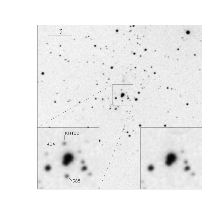
Figure 1: Digitization of a I-N/RG5 plate from 1968 Jan 21. North is up and east is left. The field of view is 20′$\times$20′, centered on the bright star HD 47887. Insets in the corners are close-ups of the region surrounding HD 47887, showing KH 15D and two of the reference stars before and after subtracting the PSF model (Eqn. 4).

We digitized these plates at Asiago Observatory using a commercial flatbed scanner with a resolution of 1600 dots per inch (dpi) and a dynamic range of 14 bits pixel^-1. The pixel scale of the digitized images is 1.53 arcseconds pixel^-1. Given the typical seeing was 6–9″, the digitized stellar images have a full width at half maximum of 4–6 pixels. The entire $5^{\circ}\times 5^{\circ}$ field of view was scanned, but for our analysis we extracted a $20\arcmin\times 20\arcmin$ subraster centered on HD 47887. A sample digitized image is shown in Figure 1.

3 Photometry

Astronomical photographic emulsions used throughout the last century typically consisted of a suspension of silver halide in a substrate of gelatin (Stock & Williams, 1962). When light strikes the halide, it produces a distribution of metallic silver grains that is made permanent by chemical development and fixation. The challenge of photographic stellar photometry is to relate the spatial distribution of the grains in a stellar image to the flux of the star.

The scanner measures $T(x,y)$, the fraction of transmitted light as a function of position on the plate. What is actually recorded is the “density distribution,”

$$d(x,y)=2^{N_{\rm bit}}\left[1-T(x,y)\right],$$ (1)

where $N_{\rm bit}=14$ is the number of bits per pixel in the digitized image. The relationship between $d(x,y)$ and stellar flux is nonlinear. In particular, for intensities above some threshold value, the density saturates. The following sections describe our method to correct for the effects of nonlinearity and saturation, and to calibrate the magnitude of KH 15D using a system of local reference stars on each plate.

3.1 Point-spread-function fitting

Our first step was to fit a parametric model to the density distribution of each star. The density distribution of faint stars is well described by a two-dimensional Gaussian function,

$$d_{G}(x,y)=d_{\rm sky}+\frac{d_{\rm peak}}{2\pi\sigma_{x}\sigma_{y}\sqrt{1-\rho^{2}}}\exp\left(-\frac{q^{2}}{2(1-\rho^{2})}\right),$$ (2)

Figure 2: Example density distributions from the plate shown in Fig. 1. The upper panels show a bright star (left) and KH 15D (right). The lower panels show the residuals after subtracting the PSF model (Eqn. 4).

where $\rho$ parameterizes the rotation and the dimensionless elliptical coordinate $q$ is defined via the equation

$$q^{2}=\frac{(x-x_{0})^{2}}{\sigma_{x}^{2}}-\frac{2\rho(x-x_{0})(y-y_{0})}{\sigma_{x}\sigma_{y}}+\frac{(y-y_{0})^{2}}{\sigma_{y}^{2}}.$$ (3)

In contrast, bright stars have a flat-topped density distribution, due to saturation. The top two panels of Fig. 2 show the density distributions of a bright star ($I\sim 9$) and the much fainter KH 15D, from the plate shown in Fig. 1. In order to accomodate a wide range of stellar magnitudes, one needs a function that changes shape with brightness. We obtained good results with a function presented by Stetson (1979),

$$d_{S}(x,y)=\left[d_{G}(x,y)^{-q}+d_{\rm sat}^{-q}\right]^{-1/q},$$ (4)

where $d_{\rm sat}$ is the saturation level of the plate, and $q$ describes the sharpness of the transition to saturation. This function has the desirable limits $d_{S}\rightarrow d_{G}$ for $d_{G}\ll d_{\rm sat}$, and $d_{S}\rightarrow d_{\rm sat}$ for $d_{G}\gg d_{\rm sat}$. It is specified by 9 parameters: $x_{0}$ and $y_{0}$; $d_{\rm sky}$ and $d_{\rm peak}$; $\sigma_{x}$, $\sigma_{y}$, and $\rho$; and the saturation parameters $d_{\rm sat}$ and $q$.

The bottom two panels of Fig. 2 show the residuals after fitting Eqn. 4 to the two example stars. In both cases the fit is excellent. For the range of stellar brightnesses considered in this paper, the peak residual was always $\lesssim$10% of the peak value of the density distribution. After fitting each star, we used the best-fitting values of the parameters to compute

$$S\equiv d_{\rm peak}\times\sigma_{x}\sigma_{y},$$ (5)

which is proportional to the volume of the density distribution above the sky level, in the limit $d_{\rm sat}\rightarrow\infty$. By computing $S$ in this manner, we attempt to correct for saturation and provide a quantity that is easily related to total stellar flux.

We selected 163 preliminary reference stars from the Flaccomio et al. (1999, hereafter F99) catalog of $BVRI$ CCD photometry of NGC 2264. Our selection criteria were that the stars should fall within the $20\arcmin\times 20$′ square region centered on HD 47887, lack close neighbor stars, and span a range of magnitudes ($12.5<I<16$) and colors ($0.5<V-I<3.0$) bracketing KH 15D ($I=14.4$, $V-I=1.6$).

For each star on each plate, we performed a nonlinear least-squares fit of Eqn. 4 to the $20\times 20$ pixel ($\approx$30$\arcsec\times 30\arcsec$) region surrounding the centroid of the density function. At first, the “plate parameters” $q$, $D_{s}$, $\sigma_{x}$, $\sigma_{y}$, and $\rho$ were determined independently for each star on a given plate. Then each plate parameter was fixed at the median of the values obtained for all stars on that plate, and the stellar fits were re-computed without varying the plate parameters. Finally, we computed $S$ for each star.

In practice, we found that KH 15D and many reference stars were well described by the simple Gaussian function (Eqn. 2). The results reported in this paper are based on the analysis using Eqn. 4, but we also repeated the analysis with the Gaussian function after dropping the brightest reference stars. None of our conclusions changed significantly.

3.2 Reduction to standard magnitudes

Next, we sought the relationship between $S$ and standard magnitudes. For the I-N/RG5 plates, we converted $S$ into Cousins $I$ using the relation

$$I=I_{0}-2.5(1+\epsilon)\log_{10}{S},$$ (6)

where $\epsilon$ represents the nonlinearity: the stellar flux is proportional to $S^{1+\epsilon}$. For each plate, we determined the values of $I_{0}$ and $\epsilon$ that minimized the sum of squared residuals between the fitted magnitudes and the F99 magnitudes. We experimented with higher-order nonlinear terms, and with color terms, but found that these were unhelpful. The residuals show no significant correlation with either magnitude or color (see Fig. 3). For most of the plates, $\epsilon$ was about 0.3.

Figure 3: The differences between fitted $I$ magnitudes and catalog (F99) $I$ magnitudes, as a function of F99 magnitude and colors. There are no significant correlations between the residuals and either color or magnitude, which is why we did not include color terms or higher-order nonlinear terms in Eqn. 6.

Many of the reference stars are cluster members which, as young stars, are likely to be variable. At this stage, we culled the most highly variable stars from the list. We computed the standard deviation $\sigma_{I}$ of each $I$ band time series, and rejected 110 stars with $\sigma_{I}>0.2$ mag. The remaining 53 stars were the final set of reference stars used to determine the magnitude of KH 15D. The choice of 0.2 mag is somewhat arbitrary; increasing the cutoff to 0.3 mag doubles the number of reference stars but has no systematic effect on the derived magnitudes of KH 15D.

Figure 4 is a color-magnitude diagram of the 53 reference stars and KH 15D, showing that KH 15D is bracketed in both color and magnitude. For each reference star, Table 1 gives the F99 catalog number, F99 $I$ magnitude, the mean $I$ magnitude measured in the Asiago plates, the difference between those two magnitudes, and $\sigma_{I}$.

Figure 4: A color–magnitude diagram for the 53 reference stars (filled circles), and KH 15D (asterisk). Data taken from F99.

For the three 103a-E/RG1 plates, we used the same set of 53 reference stars to convert $S$ into Johnson $R$ band, using a relation analogous to Eqn. 6. Likewise, for the single 103a-O/GG5 plate, we converted $S$ into Johnson $B$ band. The entries for these plates in Table 1 are estimates of $I$ under the assumption that the colors of KH 15D were $R-I=0.80$ and $B-I=2.94$, as measured by F99 (see also § 4.4).

3.3 Estimation of errors

Figure 5 is a plot of $\sigma_{I}$ vs. the time-averaged $I$ magnitude for all the reference stars. We interpret the lower envelope of the points in Figure 5 as the limiting uncertainty of our relative $I$ band measurements, as a function of magnitude. Reference stars for which $\sigma_{I}$ is much larger than this envelope are presumably variable stars. A reasonable approximation of the lower envelope is

$$\log{\sigma_{I,{\rm min}}}(I)=-0.990+0.144(I-14.4),$$ (7)

which is plotted as a dashed line in Fig. 5.

Figure 5: RMS scatter in the time series of each standard star, as a function of mean $I$ magnitude. The dashed line is our approximation $\sigma_{I,{\rm min}}(I)$ for the lower envelope.

The uncertainty in a single measurement on a given plate may be different than $\sigma_{I,{\rm min}}$, depending on the quality of that plate. One measure of plate quality is $\sigma_{m}$, the standard deviation of residuals to the fit of Eqn. 6, in magnitudes. We supposed that the uncertainty is proportional to $\sigma_{m}$. Thus, for a star with magnitude $I$ measured on a plate with fit error $\sigma_{m}$, we estimated the uncertainty to be

$${\rm Unc.}=\sigma_{I,{\rm min}}(I)\times\left(\frac{\sigma_{m}}{\sigma_{m,{\rm min}}}\right),$$ (8)

where $\sigma_{m,{\rm min}}$ is the minimum value of $\sigma_{m}$ among all the plates. For the three $R$-band measurements and the single $B$-band measurement, for which a long time series was not available, we used $\sigma_{m}$ as the estimate of uncertainty.

4 Results

The resulting $I$ band magnitudes of KH 15D are given in Table 2. Figure 6 shows the $I$ band light curve, in which there are significant variations. In the following sections we compare the Asiago light curve to the modern light curve.

Figure 6: $I$ band light curve of KH 15D from the Asiago plates. The dotted line markes the magnitude of the bright state as observed today. The error bars were computed with Eqn. 8.

4.1 Periodicity

The brightness variations were periodic in the past, as they are today. A Lomb-Scargle periodogram of the $I$ band light curve (Fig. 7) shows a highly significant peak at a period of 48.42 days, which is close to the modern period ($48.35\pm 0.02$ days; Herbst et al. 2002). To estimate the statistical uncertainty in our period determination, we used a Monte Carlo procedure. Assuming the measurement errors are Gaussian with standard deviations given by the recipe of § 3.3, we generated $10^{4}$ statistical realizations of the $I$ band light curve and determined the peak value of the periodogram in each case. The resulting distribution of periods had a standard deviation of 0.02 days. Thus, both our period and the modern period have a formal uncertainty of $\sigma=0.02$ days and differ by $3.5\sigma$, or $1.75\sigma$ in each period. This may indicate a discrepancy, but it is also quite possible that our Monte Carlo procedure underestimates the true uncertainty, due to the time evolution of the light curve.

Figure 7: Lomb-Scargle periodogram of the light curve shown in Fig. 6. Peaks above the dashed line have $<$1% chance of being a false alarm.

We computed the phase of each observation,

$$\phi=({\rm J.D.}-J_{0})\mbox{ mod }P,$$ (9)

where J.D. is the Julian date of the observation, $P=48.35$ days, and $J_{0}=2,452,690.67$, taken from the most recent ephemeris (Hamilton 2004, in preparation). Figure 8 shows the phased light curve. For comparison, we have also plotted CCD-based measurements from 2001–2002, kindly provided by C. Hamilton.

4.2 Brightness variations

In the Asiago light curve, the star alternates periodically between a bright state and a faint state. The fading events last $\approx$20 days, which is about the same duration as the 2000–2001 eclipses. However, the fractional variation in flux is much smaller in the Asiago light curve. The difference between the average magnitude in the bright state (defined as $-0.30\leq\phi\leq 0.10$) and the faint state ($0.25\leq\phi\leq 0.55$) is $\Delta I=0.67\pm 0.07$ mag. By contrast, the modern eclipse depth is 3.5 magnitudes. Interestingly, the three faintest measurements are also from the most recent time series (1979–1982; plotted with asterisks in Fig. 10), which is consistent with a progessive deepening of the eclipses.

Figure 8: Phased light curve of KH 15D from 1967-1982 (filled circles) and 2001-2002 (small dots). The solid line is a B-spline interpolation of the 2001-2002 data (see § 5).

4.3 Magnitude of the bright state

The mean magnitude of the bright state in the Asiago light curve is $I=13.57\pm 0.03$, as compared to $14.47\pm 0.03$ for the modern data. The bright state was formerly 0.90 magnitude (2.3 times) brighter than it is today. One might reasonably wonder whether this surprising discrepancy is due to an error in the zero point of our magnitude relation, or a systematic effect such as contamination by scattered light from HD 47887.

Regarding the accuracy of the zero point, Fig. 9 shows a histogram of $\Delta I$, the differences between the time-averaged magnitudes of the 53 reference stars in the Asiago plates, and the corresponding F99 magnitudes. More than 67% of the stars have $\Delta I<0.1$ mag, and the maximum $\Delta I$ is 0.3 mag. This gives us confidence that the zero point is accurate to $\approx$0.15 mag.

Regarding possible contamination, the I-N/RG5 plates were chosen precisely to minimize this problem. In the top right panel of Fig. 2, the halo of HD 47887 is evident as a small gradient in the sky level surrounding KH 15D. This gradient is too small to cause a 0.9 mag (230%) error in the estimate of the volume beneath the peak. Star 385 is even closer to HD 47887 (see Fig. 1) and has $\Delta I=-0.05$ mag. Star 404 is also within the halo of scattered light, and has $\Delta I=0.18$ mag, despite being a known variable star (Kukarkin et al., 1971).

4.4 Color variation

It would be interesting to know whether the decrease in overall brightness was accompanied by a color change. We have very limited color information, having concentrated on the I-N/RG5 plates, but the few bluer plates in our sample show no evidence for a color change. In particular, we obtained estimates of $B$ and $R$ from plates exposed less than one hour apart on 1974 December 15 (J.D. 2,439,774.6; see Table 2). The phase on this date was $\phi=0.11$, corresponding to the transition from the bright state to the faint state. The result was $B-R=2.0\pm 0.3$, in agreement with the F99 measurement, $B-R=2.14$.

Figure 9: Histogram of differences between mean $I$ magnitudes from the Asiago plates, and catalog $I$ magnitudes (F99), for the 53 reference stars. The distribution is centered near zero and has standard deviation 0.14.

4.5 Phase of minimum light

In the 30 years between the earliest group of Asiago observations and the determination of the Herbst et al. (2002) ephemeris, there have been more than 200 eclipses. The 0.02-day uncertainty in each period causes a phase uncertainty of $\Delta\phi\approx 0.1$ in the connection between the modern light curve and the Asiago light curve. Yet the phase of minimum light in the Asiago light curve occurs at $\phi_{m}=0.4$, rather than $\phi_{m}=0$ as in the modern light curve. This implies, at the 4$\sigma$ level, that there has been a shift in the phase of minimum light.

An important caveat, as mentioned in § 4.1, is that period determination for this system is difficult because the light curve does not repeat exactly from period to period. We believe it is reasonable that the period uncertainty has been underestimated, despite our best effort and the best effort of Herbst et al. 2002. This makes us reluctant to attach too much significance to the apparent phase shift before this point is clarified with additional archival data or continued monitoring.

5 Summary and discussion

The fading events of KH 15D were occurring between 1967 and 1982 with nearly the same period and duration as observed today. However, the system has changed over the past 30 years in two major respects. First, the bright state has decreased in flux by a factor of 2.3 ($0.9\pm 0.1$ mag). Second, the contrast between the bright state and the faint state has increased dramatically. Formerly, the flux of the faint state was 54% of the flux of the bright state ($\Delta I=0.67\pm 0.07$ mag). In modern observations, the corresponding figure is 4% (3.5 mag).

Interestingly, these two observations could both be explained by a time-independent flux that was present during the Asiago observations and not present during the modern observations. A steady light source with 1.3 times the flux of the eclipsing K7 star would increase the total flux by a factor of 2.3, and would also dilute the eclipses. When the K7 star is totally eclipsed, the total flux would be reduced to $1.3/2.3=57\%$ of the bright state.

To elaborate upon this idea, we created a smooth model of the 2000–2001 light curve using B-spline interpolation. This model is shown as a solid line in Figure 8. Then we considered three possible transformations of the model light curve: (1) add a constant light source of magnitude $I_{0}$; (2) shift the phase by $\Delta\phi$; and (3) stretch or compress the eclipse duration by a factor $R$. We determined the values of $I_{0}$, $\Delta\phi$, and $R$ that provide the best match to the Asiago light curve, using a nonlinear least-squares algorithm. The best fit was obtained for $I_{0}=14.11$, $\Delta\phi=0.38$, and $R=0.9$. In Figure 10, the transformed modern light curve is superposed on the Asiago data, and the residuals are plotted beneath the data. The RMS scatter of the residuals is 0.17 mag and the reduced $\chi^{2}$ is 2.1.

Figure 10: Phased light curve of KH 15D from 1967–1982, with a model based on a transformation of the 2000–2001 phased light curve (see § 5). The residuals (model$-$data) are plotted beneath the light curve.

The success of this simple model leads us to hypothesize that there is a second star in the KH 15D system. The second star was formerly blended with the $I=14.4$ K7 star seen today, but is now completely obscured. This provides an appealing explanation of the Asiago light curve but does raise an obvious question: where did the second star go?

The most economical answer, in the sense that it requires the fewest new complexities, is that the second star is currently behind the same opaque material that causes the periodic eclipses of the K7 star. The composition and arrangement of that material are unknown. Some theories are a nearly edge-on circumstellar or protoplanetary disk (Hamilton et al., 2001; Herbst et al., 2002; Winn et al., 2003; Agol et al., 2003), a dusty banana-shaped vortex (Barge & Viton, 2003), and a cometary distribution of accreting material around a low-mass companion (Grinin & Tambovtseva, 2002). The material might be distributed in such a way that one star is always hidden and the other star comes into view periodically, due to the orbital motion of the KH 15D or the circumstellar material.

If the system is truly a binary, one would expect to see radial velocity variations. Assuming the observed K7 star has a mass of $\approx$0.6 $M_{\odot}$, as estimated by Hamilton et al. 2001, and that it is in a 48-day edge-on orbit with a star of similar mass, its orbital velocity would be $\approx$30 km s^-1. This is ten times larger than the velocity shift measured by Hamilton et al. (2003) between two widely separated phases. Of course, it is possible that the full radial velocity curve shows larger variations. It is also possible that the second star is a wide binary companion, an unrelated background or foreground star, or a binary companion in a nearly face-on orbit.

Allowing the possibility of a second star to the system does not, by itself, explain the eclipses or their evolution. However, our discovery that KH 15D was brighter in the past puts two of the previous observations of this system in a different light. One of these is the result of the 1913–1951 Harvard plate analysis. Winn et al. (2003) derived limits on the fraction of time that the eclipses were $>$1 mag, but this ignored the possibility that the system was brighter at all phases in the past. The more precise statement of the result is that the system was rarely more than 1 mag fainter than the modern bright state. More speculatively, there may be a connection to the surprising observation by Kearns & Herbst (1998) that during a few of the re-brightening events, the system became brighter than the usual bright state by 0.1–0.5 mag. Perhaps during these events we were allowed a peek at the second star.

With the Asiago plates we have discovered several new clues regarding the mysterious eclipses of KH 15D, demonstrating the value of long-term preservation of astronomical images. It will be interesting to extend the historical analysis with additional plates from the 1980s and 1990s, to reveal when and how the extra light source turned off, and to complete the connection with modern data.

Table 1: Photometric reference stars in NGC 2264

F99	$I_{\rm F99}$	$I_{\rm Asiago}$	$\Delta I$	$\sigma_{I}$
Catalog No.
113	15.52	15.51	0.01	0.24
122	14.51	14.44	0.07	0.11
128	14.60	14.48	0.12	0.09
160	14.13	13.85	0.28	0.08
165	13.54	13.50	0.04	0.06
173	14.65	14.59	0.06	0.12
195	13.38	13.48	-0.10	0.09
208	13.73	13.70	0.03	0.07
227	13.39	13.30	0.09	0.11
263	13.40	13.29	0.11	0.06
272	12.57	12.57	0.00	0.06
281	13.60	13.58	0.02	0.05
289	14.94	14.95	-0.01	0.16
297	14.40	14.44	-0.04	0.11
305	13.31	13.32	-0.01	0.09
315	13.28	13.43	-0.15	0.06
320	12.88	12.94	-0.06	0.06
321	13.03	13.33	-0.30	0.12
338	13.58	13.57	0.01	0.06
342	13.94	14.10	-0.16	0.11
346	14.60	14.64	-0.04	0.11
353	13.63	13.63	0.00	0.06
364	15.21	15.27	-0.06	0.12
374	13.52	13.75	-0.23	0.11
378	14.25	14.33	-0.08	0.08
381	13.09	13.12	-0.03	0.06
385	12.91	12.96	-0.05	0.06
404	14.97	14.79	0.18	0.14
409	13.88	13.74	0.14	0.08
411	14.38	14.26	0.12	0.09
419	13.77	13.91	-0.14	0.18
422	13.66	13.67	-0.01	0.09
424	13.78	13.79	-0.01	0.06
426	13.56	13.72	-0.16	0.08
430	14.93	14.97	-0.04	0.14
431	13.01	12.97	0.04	0.07
432	14.46	14.38	0.08	0.08
434	12.98	13.07	-0.09	0.06
440	13.67	13.63	0.04	0.08
443	14.46	14.31	0.15	0.08
444	12.72	12.70	0.02	0.06
450	14.09	14.02	0.07	0.06
451	12.75	12.70	0.05	0.05
452	14.58	14.45	0.13	0.10
453	12.61	12.65	-0.04	0.06
460	13.24	13.22	0.02	0.07
462	13.54	13.48	0.06	0.05
463	12.88	12.79	0.09	0.06
481	13.40	13.45	-0.05	0.07
504	13.55	13.53	0.02	0.06
512	14.14	14.15	-0.01	0.10
515	12.68	12.78	-0.10	0.07

Table 2: Photometric Measurements of KH 15D

J.D.	$\phi$	I
2439530.46	0.8121	$13.46\pm 0.08$
2439763.22	0.6261	$13.43\pm 0.08$
2439765.65	0.6762	$13.7\pm 0.1$
2439769.65	0.7591	$13.45\pm 0.08$
2439771.58	0.7989	$13.5\pm 0.1$
2439772.56	0.8192	$13.47\pm 0.09$
2439773.59	0.8405	$13.5\pm 0.1$
2439774.62	0.8619	$13.44\pm 0.09$
2439774.67	0.8628	$13.5\pm 0.1$
2439775.63	0.8826	$13.49\pm 0.09$
2439796.57	0.3157	$14.09\pm 0.08$
2439826.67	0.9384	$13.6\pm 0.1$
2439827.66	0.9588	$13.5\pm 0.1$
2439831.69	0.04213	$13.7\pm 0.1$
2439852.63	0.4753	$14.1\pm 0.1$
2439860.58	0.6396	$13.60\pm 0.08$
2439876.33	0.9655	$13.50\pm 0.09$
2439877.33	0.9862	$13.53\pm 0.06$
2439878.48	0.009931	$13.5\pm 0.1$
2439878.52	0.01074	$13.45\pm 0.09$
2439879.30	0.02694	$13.47\pm 0.09$
2439881.51	0.07251	$13.5\pm 0.1$
2439885.53	0.1556	$13.82\pm 0.09$
2439887.50	0.1965	$13.9\pm 0.1$
2439905.46	0.5680	$13.7\pm 0.1$
2439943.30	0.3506	$14.0\pm 0.1$
2439947.31	0.4335	$14.0\pm 0.1$
2440127.66	0.1636	$13.7\pm 0.1$
2440241.49	0.5178	$13.73\pm 0.09$
2440264.25	0.9886	$13.65\pm 0.08$
2440273.28	0.1753	$13.9\pm 0.1$
2440274.44	0.1994	$14.0\pm 0.1$
2440479.66	0.4439	$14.3\pm 0.1$
2440485.66	0.5679	$14.0\pm 0.1$
2440509.67	0.06442	$13.9\pm 0.1$
2440569.55	0.3030	$14.3\pm 0.1$
2440588.51	0.6951	$13.64\pm 0.09$
2440589.58	0.7172	$13.5\pm 0.1$
2440621.55	0.3785	$14.3\pm 0.1$
2440626.32	0.4772	$14.3\pm 0.1$
2440647.35	0.9121	$13.6\pm 0.2$
2441960.64	0.07422	$13.6\pm 0.1$
2442373.51	0.6135	$14.0\pm 0.2$
2442396.49	0.08877	$13.4\pm 0.2$
2442397.49	0.1093	$13.3\pm 0.2$
2442397.50	0.1095	$13.6\pm 0.2$
2442816.44	0.7744	$13.60\pm 0.08$
2444202.51	0.4418	$14.6\pm 0.2$
2444292.42	0.3013	$14.4\pm 0.2$
2444609.31	0.8555	$13.7\pm 0.1$
2444642.49	0.5417	$14.5\pm 0.2$
2445002.48	0.9872	$13.8\pm 0.1$

References

- Agol et al. (2003) Agol, E., Barth, A.J., Wolf, S., & Charbonneau, D. 2003, preprint [astro-ph/0309309]
- Barbieri, Omizzolo, & Rampazzi (2003) Barbieri, C., Omizzolo, A., & Rampazzi, F. 2003, Memorie della Societa Astronomica Italiana, 74, 430
- Barge & Viton (2003) Barge, P. & Viton, M. 2003, ApJL, 593, L117
- Flaccomio et al. (1999) Flaccomio, E., Micela, G., Sciortino, S., Favata, F., Corbally, C. & Tomaney, A. 1999, A&A, 345, 521
- Grinin & Tambovtseva (2002) Grinin, V. P. & Tambovtseva, L. V. 2002, Ast. Lett. 28, 601
- Hamilton et al. (2001) Hamilton, C.M., Herbst, W., Shih, C., & Ferro, A.J. 2001, ApJ, 554, L201
- Hamilton et al. (2003) Hamilton, C. M., Herbst, W., Mundt, R., Bailer-Jones, C. A. L., & Johns-Krull, C. M. 2003, preprint [astro-ph/0305477]
- Herbst et al. (1994) Herbst, W., Herbst, D.K., Grossman, E.J. & Weinstein, D. 1994, AJ, 108, 1906
- Herbst et al. (2002) Herbst, W., Hamilton, C.M., Vrba, F.J., Ibrahimov, M.A., Bailer-Jones, C.A.L., Mundt, R., Lamm, M., Mazeh, T., Webster, Z.T., Haisch, K.E., Williams, E.C., Rhodes, A.H., Balonek, T.J., Scholz, A. & Riffeser, A. 2002, PASP, 114, 1167 [H02]
- Kearns & Herbst (1998) Kearns, K. E. & Herbst, W. H. 1998, AJ, 116, 261
- Kukarkin et al. (1971) Kukarkin, B.V., Kholopov, P.N., Pskovsky, Y.P., Efremov, Y.N., Kukarkina, N.P., Kurochkin, N.E. & Medvedeva, G.I., in General Catalog of Variable Stars, 3rd ed. (1971)
- Moro & Munari (2000) Moro, D. & Munari, U. 2000, A&AS, 147, 361
- Stetson (1979) Stetson, P.B. 1979, AJ, 84, 1056
- Stock & Williams (1962) Stock, J. & Williams, A.D. 1962, Photographic Photometry (University of Chicago Press), 374–423
- Winn et al. (2003) Winn, J.N., Garnavich, P.M., Stanek, K.Z., & Sasselov, D.D. 2003, ApJL, 593, L121