Testing for a Super-Acceleration Phase of the Universe

Abstract

We propose a method to probe the phenomenological nature of dark energy which makes no assumptions about the evolution of its energy density. We exemplify this method with a test for a super-acceleration phase of the universe i.e., a phase when the dark energy density grows as the universe expands. We show how such a phase can be detected by combining SNIa (SNAP-like) and CMB (Planck) data without making any assumptions about the evolution of the dark energy equation of state, or about the value of the matter density parameter.

I Introduction

Observations of distant Type Ia supernovae imply a presently accelerating universe riess98 ; perlmutter99 . In the standard cosmological model this is accommodated by introducing “dark energy”, a component which interacts with the rest of the universe only gravitationally and has a significantly negative pressure which leads to the acceleration of the universe.

In order to accelerate the universe, the dark energy component must have an energy density which decreases (if at all) much more slowly than matter density as the universe expands. Current data favor a dark energy density which is almost constant or increasing with time caldwell99 ; schuecker02 ; tonry03 ; knop03 ; choudhury03 ; alam03 and exciting results can be expected in the future weller01 ; frieman02 ; linder03 ; kratochvil03 . We label the phase when the dark energy density is increasing with the expansion of the universe as super-acceleration.

In this paper we discuss a method to probe phenomenological properties of dark energy without any assumptions about the evolution of dark energy density. We use this method to formulate a test to ascertain if the universe evolved through a super-acceleration phase by combining SNIa and CMB experiments. We quote our results in terms of two variables $\bar{w}_{\rm sn}$ and $\bar{w}_{\rm cmb}$ which are the best fit constant dark energy equation of state parameters for the SNIa and CMB experiments respectively. Our method does not rely on the equation of state parameter being constant. In fact, we do not need to assume anything about the evolution of the dark energy equation of state, or about the value of the matter density parameter.

We will outline our method in the context of the specific example of testing for super-acceleration using SNIa and CMB experiments. We will end with a discussion of how our method can be generalized to other questions one might ask about dark energy using SNIa, CMB and other experiments. Questions of the nature, “did the dark energy density increase with cosmic expansion?” are perhaps easier to answer than some questions previously asked in the literature. And yet they have the potential to revolutionize our thinking about dark energy. We stress that answering such questions does not necessarily require measuring the complete dark energy density evolution; the key point is that we are asking for less information.

In a nutshell, to apply this method one needs to fit a constant equation of state $\bar{w}$ to each of SNIa and CMB observations and plot conditional probabilities in the $\bar{w}$ versus $\Omega_{M}$ plane (e.g., Fig. 1). The probabilities are conditional in the sense that they are normalized at each value of $\Omega_{M}$. If the upper contours cross below $\bar{w}=-1$ then super-acceleration has been detected. We stress that the power to make such robust statements comes from combining different measures (SNIa and CMB) which have complementary dependencies on the dark energy equation of state and matter density.

In Section II we start with a discussion of dark energy and define super-acceleration rigorously. We then outline the general characteristics of models which could describe a super-acceleration phase. Given that dark energy is a total mystery even if it never went through a super-acceleration phase, our point of view is that super-acceleration is a question to be observationally settled. It is satisfying to note that this will be possible with upcoming experiments. We explain our evolution-independent method in Section III. We then proceed to forecast the possibilities with regard to measuring a super-acceleration phase from future missions in Section IV. We end with a discussion of how the method can be generalized.

II Dark Energy and Super-Acceleration

In this section we will consider dark energy in a general setting (without reference to a theory of gravity) and define it in terms of its phenomenological properties. This will allow us to motivate super-acceleration as a part of phenomenologically viable parameter space. Finally, we will consider some models where a super-acceleration phase might arise. These models are discussed with an aim to better understand the requirements that super-acceleration imposes.

II.1 Generalized Equation-of-state

The pressure of the dark energy (DE) $p_{X}$ is parameterized in terms of the equation of state $w_{X}$ which relates it to the physical energy density $\rho_{X}$ as $p_{X}=w_{X}\rho_{X}$. In terms of $w_{X}$ the evolution of the DE density with scale factor $a$ is $\rho_{X}(a)\propto\exp(-3\int^{a}d\ln a^{\prime}(1+w_{X}(a^{\prime}))$. If $w_{X}<-1$, then the DE density is actually increasing as the universe expands, which seems counter-intuitive. In the context of a scalar field ($\phi$) with canonical kinetic ($\dot{\phi}^{2}/2>0$) and potential ($V(\phi)>0$) terms, $w_{X}<-1$ is unphysical. This is easily seen by rewriting $w_{X}$ as $1+w_{X}=2\dot{\phi}^{2}/[\dot{\phi}^{2}+2V(\phi)]$ which is positive if $V(\phi)>0$.

The SNIa observations provide us with a magnitude–redshift relationship. If the SNIa can be standardized as sources with known luminosity, then they measure the luminosity distance $d_{L}(z)$ in units of $1/H_{0}$ where $H_{0}$ is the present expansion rate of the universe. Within the context of homogeneous and isotropic universes, we can then write

$$D(z)\equiv{H_{0}d_{L}(z)\over(1+z)}=\int_{0}^{z}{dz\over h(z)}\,,$$ (1)

where $h(z)=(\dot{a}/a)/H_{0}$ is the expansion rate of the universe normalized to unity today and $z=1/a-1$ is the redshift. Acceleration refers to the condition $\ddot{a}>0$. We can parameterize the expansion rate as

$$h^{2}(z)=(1+z)^{3}\left[\Omega_{M}+\Omega_{X}\exp(3\int_{0}^{z}d\xi\,w_{X}(\xi)/(1+\xi))\right].$$ (2)

This is completely general and it does not tie us down to a theory of gravity (see tegmark01 ; carroll01 ; linder02 ; dvali03 ; linder03 for examples of studying cosmology in this spirit). Any $h(z)$ can be written in terms of $w_{X}(z)$ as above. Eq. 2 is a phenomenological fit; we need a theory (for gravity, dark matter and dark energy) to interpret $\Omega_{M}$ and $w_{X}(z)$.

We can differentiate Eq. 2 to derive the acceleration of the scale factor. This yields

$$2\ddot{a}/a=-(1+3w_{X}(z))h^{2}(z)+3w_{X}(z)(1+z)^{3}\Omega_{M}\,.$$ (3)

The universe is accelerating if $w_{X}(0)<-1/[3(1-\Omega_{M})]$. Also, for $-1/[3(1-\Omega_{M})]>w_{X}(0)>-1/(1-\Omega_{M})$ we have $\ddot{a}(0)>0$ but $\dot{h}(0)<0$.

II.2 Super-Acceleration

We will refer to an expansion phase with $w_{X}(z)<-1$ as super-acceleration . Super-acceleration implies that the dark energy contribution to the expansion rate is increasing with time and this leads to interesting scenarios for the ultimate fate of the universe mcinnes01 ; caldwell03 . In particular, it is possible that the universe could end in a “Big-Rip”, with the time scale for such catastrophic events set by $1/H_{0}$. In order to draw such conclusions, the future evolution of $w_{X}(z)$ must be known.

We are interested in the issue of whether future observations will be able to ascertain that the universe went through a super-acceleration phase. The main motivation for thinking about super-acceleration is the simple fact about dark energy – we don’t know what it is. Given our current understanding, even if we know what $w_{X}(z)$ exactly is, dark energy will still be a mystery.

One of the troubling things about super-acceleration is that it seems to violate causality. The magnitude of the pressure is larger than the energy density and hence one might expect to transmit information faster than the speed of light. While this is a possibility, it is by no means guaranteed by having $|p_{X}|>\rho_{X}=3{\rm m}_{\rm pl}^{2}H_{0}^{2}[h^{2}(z)-(1+z)^{3}\Omega_{M}]$. $w_{X}(z)$ determines the global evolution of $\rho_{X}$; it does not tell us how small local perturbations propagate.

II.3 Modeling Super-Acceleration

Given the repercussions and the unintuitive nature of $w_{X}(z)<-1$ systems, it is of interest to investigate models which give rise to a super-acceleration measurement.

1. One possibility is that the universe is accelerating due to a cosmological constant (or perhaps some dynamical scalar field), but the effective $w_{X}$ at some epoch goes below -1 because of new physics we are unaware of. An example of new physics kaloper03 could be the coupling of photons to axions (not the QCD axion) csaki01 which has been proposed to explain the dimming of supernovae without the need for an accelerating universe.

2. A second (troubling) possibility is that the effective $w_{X}$ is less than -1 because of systematic effects. This is similar to (1) except it is not new physics but some systematic effect that results in the “apparent” super-acceleration.

3. $w_{X}<-1$ is a possibility if one postulates that dark energy is a scalar field with non-canonical kinetic terms caldwell99 ; picon99 ; chiba99 ; frampton02 . One must be careful about instabilities in the theory in this case carroll03 .

4. Another class of models appeals to a modification of gravity on scales $\mathrel{\mathchoice{\lower 3.6pt\vbox{\halign{$\mathsurround=0pt\displaystyle\hfil#\hfil$\cr<\crcr\sim\crcr}}}{\lower 3.6pt\vbox{\halign{$\mathsurround=0pt\textstyle\hfil#\hfil$\cr<\crcr\sim\crcr}}}{\lower 3.6pt\vbox{\halign{$\mathsurround=0pt\scriptstyle\hfil#\hfil$\cr<\crcr\sim\crcr}}}{\lower 3.6pt\vbox{\halign{$\mathsurround=0pt\scriptscriptstyle\hfil#\hfil$\cr<\crcr\sim\crcr}}}}1/H_{0}$ to obtain $w_{X}(z)<-1$. Like the other models in this section, this class of models does not solve the “why now?” problem since the scale $H_{0}$ is put in by hand to make sure that gravity is only modified today. There are severe constraints on modified gravity theories in the early universe carroll01 . The main impetus for considering modified gravity theories is provided by brane-world models wherein it might be possible to get super-acceleration sahni02 ; dvali03 .

III Detecting Super-Acceleration

In this section we lay out the method by which future experiments can unambiguously detect a super-acceleration phase, independent of the functional form of $w(z)$. First we show that if a constant equation of state is fitted to SNIa observations and a result less than $-1$ is obtained then either the true equation of state must at some point dip below $-1$, or the assumed matter density is incorrect. We then show the same thing for CMB observations. Finally we show how SNIa and CMB information together can overcome the need to assume a value for the matter density. Throughout we assume a flat universe.

III.1 Information from Supernova observations

Given a set of SNIa observations our method uses conventional $\chi^{2}$ fitting to obtain the best fitting constant equation of state for each $\Omega_{M}$ (see next section). The aim of the following paragraphs is to show the significance of this fitted constant equation of state, given that the actual equation of state is of unknown functional form.

A SNIa experiment measures the luminosity distance $D_{E}$ out to a certain set of redshifts. As usual, we define:

$$D_{E}(z)={1\over\sqrt{\Omega_{M}}}\int_{0}^{z}{dz\over\sqrt{(1+z)^{3}+r_{E}(z;\Omega_{M})}}\,,$$ (4)

where $r_{E}(z;\Omega_{M})\equiv(\Omega_{X}/\Omega_{M})\exp[3\int_{0}^{z}dz^{\prime}(1+w_{X}(z^{\prime}))/(1+z^{\prime})]$. The subscript $E$ in Eq. 4 explicitly denotes that this is the quantity measured by an experiment. We are further assuming that the experimental magnitude redshift relation is an unbiased estimator of the actual luminosity distance.

The next step in our method is to fit the distance $D_{E}(z)$ with a distance $D_{F}(z,\Omega_{M},\Delta w)$ which assumes a constant equation-of-state, $w_{X}(z)=\bar{w}_{\rm sn}=-1+\Delta w$. Thus $D_{F}$ is has the same form as $D_{E}$ but with $r_{E}$ replaced by $r_{F}(z;\Omega_{M})=(\Omega_{X}/\Omega_{M})(1+z)^{3\Delta w}$. The best-fit $\Delta w$ is found by maximizing the likelihood assuming gaussian errors (appropriate for SNAP) for the measured distances.

We give a more rigorous derivation in the following paragraphs, but to gain a qualitative understanding first consider the weighting function approach of Saini et. al. saini03 . They showed that to a good approximation a constant fitted equation of state from supernovae observations is simply a weighted average over redshift of the true equation of state, where the weighting function is always positive. From this it is clear that if the constant fitted equation of state is less than $-1$ then the true equation of state must also go below $-1$ for some redshift interval(s). The above is only true if the correct matter density has been assumed.

We now have the task of computing the best-fit $\Delta w$ for a given $D_{E}(z)$ at a fixed $\Omega_{M}$. This is found by minimizing the $\chi^{2}$ at fixed $\Omega_{M}$ with respect to $\Delta w$. The resulting equation does not have a simple solution. Our aim is to figure out when the best-fit $\Delta w<0$. To achieve this, we replace $D_{F}$ in the minimization equation by its a first order Taylor expansion in $\Delta w$, i.e.,

$$D_{F}(z,\Omega_{M},\Delta w)\simeq D_{\Lambda}(z,\Omega_{M})+\Delta w\,G_{\Lambda}(z,\Omega_{M})\,.$$ (5)

$D_{\Lambda}$ is defined the same way as $D_{F}$ but with $\Delta w=0$, i.e., $D_{\Lambda}(z,\Omega_{M})$ is the distance in $\Lambda$CDM cosmology. We define $G_{F}=dD_{F}/d\Delta w$ and the function $G_{\Lambda}(z,\Omega_{M})=G_{F}(z,\Omega_{M},\Delta w=0)$. For $\Omega_{M}>0.1$ and $0<z<1.7$, the error in the approximation given by Eq. 5 is smaller than 3% for $-0.5<\Delta w<0.5$. We note that Saini et. al. saini03 have shown that this kind of linear approximation works extremely well even when $\Delta w$ is not constant (in which case we need to take a functional derivative with respect to $\Delta w(z)$.)

We note three facts. One, we are only approximating the fit (to ascertain whether $\Delta w<0$) and not making any assumptions about the actual $w_{X}(z)$.

Two, the error in approximating $D_{F}$ according to Eq. 5 turns out to be unimportant. At the end of this section, we show explicitly that the only effect of this approximation is to make our results (on detecting super-acceleration) somewhat conservative.

Three, we could just as well use $D_{F}=D_{\Lambda}+\Delta wG_{\Lambda}$ as our exact fit and it would not change any of our arguments. We chose not to go this route because the above fit is unintuitive and has unphysical behavior for large $\Delta w$.

Applying the approximation in Eq. 5 to the equation resulting from the minimization procedure, we get the following implicit equation for the best-fit $\Delta w$:

$$\Delta w=\frac{\Sigma_{i}\,\left[D_{E}(z_{i})-D_{\Lambda}(z_{i},\Omega_{M})\right]G_{F}(z_{i},\Omega_{M},\Delta w)/\sigma^{2}(z_{i})}{\Sigma_{i}\,G_{F}(z_{i},\Omega_{M},\Delta w)G_{\Lambda}(z_{i},\Omega_{M})/\sigma^{2}(z_{i})}.$$ (6)

Both $G_{F}$ and $G_{\Lambda}$ are negative for all $z$. What Eq. 6 says is that if the best fit $\Delta w<0$, then $D_{E}(z_{i})>D_{\Lambda}(z_{i},\Omega_{M})$ for a finite number of $z_{i}$ or $\Omega_{M}$ is wrong. This in turn implies that if $\Omega_{M}$ is the true value, then $w_{X}(z)$ must be less than -1 for some redshift range.

A point of note here is that for each $\Omega_{M}$ we have a corresponding best-fit $\Delta w(\Omega_{M})$. We are not minimizing with respect to both $\Omega_{M}$ and $\Delta w$. The $\Omega_{M}$ resulting from a joint minimization need not be the true matter density and in fact it could be that the best-fit $\Delta w<-1$ even though the underlying $w_{X}(z)$ never enters a super-acceleration phase maor01 .

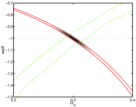
Figure 1: The shading shows the two-dimensional probability distribution from SNAP-type supernova data in the $\bar{w}_{\rm sn}$–$\Omega_{M}$ plane. The solid lines show 68 per cent limits at each $\Omega_{M}$ from the same simulated data. The dashed lines show 68 per cent limits at each $\Omega_{M}$ from a Planck-type simulation, marginalized over 5 other cosmological parameters. The input model has $\Omega_{M}=0.3$ and $w(z)=-1$ (a constant).

How are our results affected by the small error in approximating the fit luminosity distance $D_{F}$ by a first order Taylor expansion? To answer this question let us write

$$D_{F}(z,\Omega_{M},\Delta w) = (D_{\Lambda}(z,\Omega_{M})+\Delta w\,G_{\Lambda}(z,\Omega_{M}))$$ (7)

$$\times (1-\epsilon(z,\Omega_{M},\Delta w))\,.$$

For the interesting parameter space, $\epsilon(z,\Omega_{M},\Delta w)$ is smaller than about 0.03. Further, for all practical purposes, this approximation overestimates $D_{F}$. One can then show that the effect of this is to make $\Delta w$ smaller. Thus the conclusions drawn from Eq. 6 are conservative in the sense that $\Delta w$ is more negative than what we would find from Eq. 6.

An interesting exercise is to fit the supernova distances with $D_{F}(z,\Omega_{M},\Delta w)=D_{\Lambda}(z,\Omega_{M})+\Delta w\,G_{\Lambda}(z,\Omega_{M})$ exactly. We can then run through the same arguments as before and arrive at the same conclusion. In particular, we computed the new contours with $w_{\rm sn}\equiv-1+\Delta w$ and the quantitative results changed very little as expected.

III.2 Low redshift supernova calibration

In the discussion above, we have assumed that we can measure luminosity distance $D_{L}$ as a function of redshift from supernovae. However in practice we can only measure magnitudes $m$

$$m=\mathcal{M}+5\log D_{L}(z,\Omega_{m},w(z))\,,$$ (8)

where the calibration factor $\mathcal{M}$ is unknown unless we have a very large number of low redshift supernovae.

We expect a few hundred supernovae from SNFactory aldering02 and the low redshift Carnegie Supernova Program phillips04 and that will enable calibration of the luminosity distances to around 0.5 per cent. If the $\sim$6000 supernovae that should be seen by GAIA belokurov03 were all followed up then this could reduce the uncertainty to 0.2 per cent.

This additional uncertainty will reduce our ability to determine if super-acceleration occurred. We take the conservative (and not fully optimized) approach of assuming the worst possible value for the calibration parameter and feeding it through the analysis described above. If the luminosity distance calibration were actually a factor of 1.015 (3$\times$0.5 per cent) higher than estimated from the low redshift sample, then the supernova contours would shift from the solid lines in Fig. 2 to the dotted lines. This factor corresponds to the true calibration factor being about three $\sigma$ away from that estimated by the upcoming experiments. If there were significantly more supernovae followed up, then this would improve the picture. For example, we get the dashed contour with a factor of 1.006.

III.3 Information from CMB observations

The CMB is sensitive to the dark energy mainly through its effect on the angular diameter distance to the CMB, and therefore the positions of the acoustic peaks huey98 . It also has an effect on the largest scales since dark energy changes the Integrated Sachs Wolfe effect, through both the change in the expansion rate and clustering. Here we propose to ignore the CMB information on large scales so that there is no need to make assumptions about the clustering of dark energy.

In the case of the CMB, the approximation given in Eq. 5 does not work well. However we do not need the approximation since the CMB measures the angular diameter distance out to just one redshift, that of the last scattering surface. The equation to solve for the CMB is $D_{F}(\infty,\Omega_{M},\Delta w)=D_{E}(\infty)$ (neglecting the small error on $D_{E}$). Although the relation between $\Delta w$ and $D_{E}(z)$ is non-trivial here, the argument is simple. For the true $\Omega_{M}$ if the relation $D_{F}(z,\Omega_{M},\Delta w)=D_{E}(z)$ implies that $\bar{w}_{\rm cmb}\equiv-1+\Delta w<-1$ then a super-acceleration phase must happen over a finite range of redshift. This is simply a consequence of the fact that $D_{F}(z,\Omega_{M},\Delta w)$ is a monotonically decreasing function of $\Delta w$.

Qualitatively, when a constant equation of state is fitted to CMB data it measures roughly a weighted average of the true $w_{X}(z)$ where the weighting function is always positive saini03 . Therefore if the fitted $\bar{w}_{\rm cmb}$ gives a value less than $-1$ then the true equation of state must itself dip below $-1$. As for the SN1a argument, this is only true if the value of $\Omega_{M}$ has been guessed correctly.

III.4 Combination

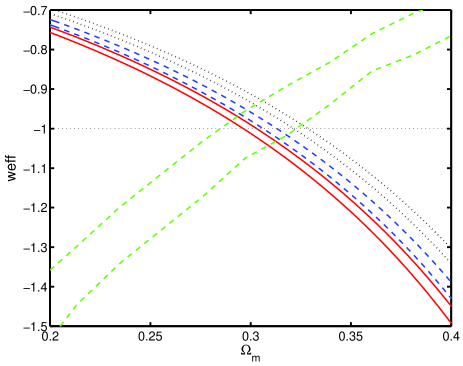
Figure 2: The contours in this figure are computed the same way as the contours in Fig. 1. The solid supernova contour assumes that the calibration error is negligible. The dashed lines are 68 % limits assuming a worst case calibration parameter estimated from 6000 low redshift supernovae. The dotted line is the same as the dashed but for 300 low redshift supernovae.

As discussed above, using SNIa alone it is not possible to uncover the nature of dark energy simultaneously with estimating the matter content $\Omega_{M}$. This is also true for CMB data alone. Therefore we need to combine information from SNIa and CMB. Given observed data we can determine the limits on $\bar{w}$ at each $\Omega_{M}$ for both SNIa and CMB and plot this conditional likelihood in the $\bar{w}$–$\Omega_{M}$ plane. In general the best-fit $\bar{w}$ at some $\Omega_{M}$ derived from SNIa will be different from that derived from CMB since they probe the equation of state at different redshifts. For illustration we use contours which encapsulate 68% of the likelihood throughout, however the method can be carried out for whatever confidence level is required.

The key point of our argument is that if, for every value of $\Omega_{M}$, the contour for either $\bar{w}_{\rm cmb}$ or $\bar{w}_{\rm sn}$ falls below -1, then it must be that dark energy went through a phase of super-acceleration for a finite period of time. We explain how this follows from the previous sections by discussing two examples.

Consider the example in Fig. 1. Suppose that we do not know the true value of $\Omega_{M}$. We get around this problem by considering each possible value for $\Omega_{M}$ in turn. For each $\Omega_{M}$ value we assess whether, if this were indeed the true value of $\Omega_{M}$, we would conclude that the universe underwent super-acceleration. If for all values of $\Omega_{M}$ we reach the same conclusion, then we can give a definitive answer, independent of the value of $\Omega_{M}$.

As an example let us first consider the value $\Omega_{M}=0.2$. In this case $\bar{w}_{\rm sn}>-1$ and $\bar{w}_{\rm cmb}<-1$. If this were the true value of $\Omega_{M}$ then we would have to conclude that at some point in the history of the universe, $w(z)<-1$. (In fact since the CMB probes the value of $w(z)$ at higher redshifts than SNIa then this would imply that $w$ was once less than $-1$ and has since risen above $-1$, but these details are not important for our argument.) We would reach this same conclusion for all matter densities with $\Omega_{M}\lower 2.15277pt\hbox{$\;\buildrel<\over{\sim}\;$}0.28$. Now consider the value $\Omega_{M}=0.4$. If this were the true value of $\Omega_{M}$ then we would again conclude that for some redshifts $w(z)<-1$, since $\bar{w}_{\rm sn}<-1$. We would reach the same conclusion for $\Omega_{M}\lower 2.15277pt\hbox{$\;\buildrel>\over{\sim}\;$}0.305$. However, for $\Omega_{M}=0.3$ then both data sets allow $\bar{w}>-1$, therefore we cannot be sure whether or not there was super-acceleration. Our conclusion from Fig. 1 is that either $0.28\lower 2.15277pt\hbox{$\;\buildrel<\over{\sim}\;$}\Omega_{M}\lower 2.15277pt\hbox{$\;\buildrel<\over{\sim}\;$}0.305$ or there was super-acceleration.

Now consider future observations providing the solid (SNIa) and dashed (CMB) lines in Fig. 4. Running through the same arguments as above, we conclude that, no matter what the value of $\Omega_{M}$, there must have been super-acceleration. This can be seen at a glance by the fact that the upper contours cross below $-1$.

The method we have just outlined determines if the universe underwent a super-acceleration phase without any assumptions about the evolution of dark energy density. It is clear from the above discussion that one cannot test for a super-acceleration phase if the deviation from $w_{X}=-1$ is arbitrarily tiny. How well can we do with future experiments? We turn to this question next.

IV Forecasts

In order to make a prediction about how well future experiments will do, we need to generate mock data ($D_{E}$) which in turn requires that we make some assumptions about the evolution of $w_{X}(z)$. This is not a major hurdle (as we show later), mostly because we interested in getting a rough sense of what future experiments can achieve. In the next section, we will discuss the procedure used to generate mock data assuming a particular $w_{X}(z)$ function. We generate data relevant for SNAP-like and Planck experiments.

IV.1 SNIa data

We assume that the luminosity distance will be measured to an accuracy of 1.4 per cent in each of 50 redshift bins evenly spaced between redshift 0.1 and 2. First we simulate data from a model with $w(z)=-1$ and $\Omega_{M}=0.3$.

On fitting the two parameters, $\bar{w}_{\rm sn}$ and $\Omega_{M}$ we obtain a tight constraint on the two parameters indicated by the shading in Fig. 1.

For our method the quantity of interest is not the two-dimensional probability (as shown by the shaded contour) but the confidence limits on $\bar{w}_{\rm sn}$ calculated for a given $\Omega_{M}$. These limits are shown by the solid lines on Fig. 1 and as expected the contours extend to $\bar{w}_{\rm sn}<-1$ in the direction of increasing $\Omega_{M}$.

IV.2 CMB data

We generate CMB temperature anisotropy (TT) data using the parameters for the Planck HFI 353 GHz channel: sensitivity $\Delta T/T=14.4\times 10^{-6}$, solid angle per pixel $4\pi/5.94\times 10^{6}$ (where $5.94\times 10^{6}$ is the number of pixels on the sky) and 5 arcmin FWHM beam and assume 100 per cent of the sky can be used. To speed up the computation we bin the observations with $\Delta\ell=10$ and go up to $\ell_{\rm max}=2500$. We also marginalize over the Hubble constant, the baryon content, and the amplitude and spectral index of the primordial scalar fluctuations. We ignore tensor modes and do not use CMB polarization information, although in principle these could both be included in the analysis.

The CMB data essentially constrain the angular diameter distance to last scattering $z\sim 1100$ and therefore there is a perfect degeneracy between $\bar{w}_{\rm cmb}$ and $\Omega_{M}$. Including the large scale ISW effect (the decay of gravitational potential due to dark energy domination) or lensing on small scales would break this degeneracy to some extent. However, a reliable estimation of the degeneracy breaking would require some assumptions about the clustering of dark energy. In light of the uncertain nature of the models of dark energy with $w_{X}(z)<-1$, we have decided to not use the lensing signal or the $\ell<50$ power spectrum (where the ISW effect is important). We again plot contours at the 68 per cent confidence limits for each $\Omega_{M}$ value, although the more conventional contours at constant two-dimensional probability look similar.

IV.3 Requirements on w(z) for detection

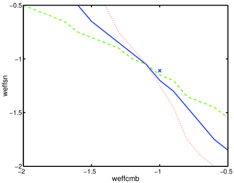
Figure 3: The value of $\bar{w}_{\rm sn}$ below which it is possible to detect super-acceleration, for a given $\bar{w}_{\rm cmb}$ and $\Omega_{M}$. The solid curve corresponds to a fiducial matter density of $\Omega_{M}=0.3$, the dashed line corresponds to $\Omega_{M}=0.2$ and the dotted line corresponds to $\Omega_{M}=0.4$. The cross shows the $\bar{w}_{\rm sn}$ at which super-acceleration can be detected for an evolving equation of state with a jump in $w_{x}(z)$ at redshift 0.3 for $\Omega_{M}=0.3$.

In the simplest approximation the shape of the contours in Fig. 1 is independent of the shape of $w_{X}(z)$. For now we assume this to be true and assume the shape is the same as that for a constant $w_{X}$. We discuss the validity of this approximation in the following subsection.

We produce plots similar to Fig. 1 but simulate data for models with various values for the constant equation of state. We fix $\Omega_{M}=0.3$ throughout and allow different values for the equation of state for the CMB simulations and the SNIa simulations. This corresponds to the case where the equation of state is varying with redshift and therefore the effective value is different for the two probes. For each assumed $\bar{w}_{\rm cmb}$ we calculate the $\bar{w}_{\rm sn}$ for which the upper CMB and SNIa 68% contours cross below $-1$, and therefore it is possible to detect super-acceleration. This is shown by the solid line in 3. For this value of $\bar{w}_{\rm sn}$ and lower it is possible to detect super-acceleration. The dashed and dotted lines show the equivalent for $\Omega_{M}=0.2$ and $\Omega_{M}=0.4$.

This takes into account the error bars predicted for SNAP-like and Planck-like experiments. For example, if the true value of $\Omega_{M}$ is 0.3 then if we measure $\bar{w}_{\rm cmb}=-1$ then $\bar{w}_{\rm sn}$ must be less than $-1.3$ if we are to detect super-acceleration from these future experiments. Note that it is not necessary for us to assume a value for $\Omega_{M}$ in order to detect super-acceleration; however the true value of $\Omega_{M}$ will affect how easy it would be to detect such a phase.

In making Fig. 3, we have assumed that the calibration error is negligible. Depending on the calibration error, the curves in Fig. 3 will shift down somewhat. The magnitude of this effect may be ascertained by looking at the shift of the contours in Fig. 2.

IV.4 Insensitivity to assumed fiducial $w_{X}$

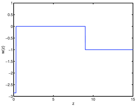
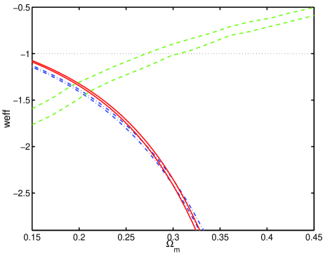
Figure 4: (a) The equation of state as a function of redshift for an extreme strongly evolving model. A large jump occurs at $z=0.3$. (b) Solid blue lines: 68 per cent confidence limits on $\bar{w}_{\rm sn}$ for each $\Omega_{M}$ value from a SNAP-type simulation with w(z) given by Fig. 3(a). Dash-dot lines: the simulation has $w(z)=-2.38$, the best fitting constant equation of state model to the supernova data. The solid and dash-dot lines are quite similar, despite the fact that the $w_{X}$ evolution is so different in the two cases. Since this w(z) was devised to give the same angular diameter distance to the CMB as a $w=-1$ model, the CMB contours (dashed lines) are unchanged from Fig. 1.

To calculate the lines in Fig. 3 we assumed that the shape of the contours (e.g., of Fig. 1) are independent of the form of $w(z)$. We take two approaches to assess the reliability of this approximation. First we calculate the mathematical requirements for this approximation to be true. Then we take an extreme example of a sharply changing $w(z)$ and show how even in this case, our predictions in Fig. 3 are not altered much.

To determine the mathematical requirements for our approximation let us assume we simulate mock data with a given value of matter density denoted by $\Omega_{M}^{t}$ (“true matter density”) and a particular evolution for the dark energy density. For this $D_{E}(z)$ we find the best fit $\bar{\Delta}w(\Omega_{M})$ (as described above in Section III). We are interested in the question of how $\Delta w(\Omega_{M})$ changes due to a change in $D_{E}(z)$ with the constraint that $\Delta w(\Omega_{M}^{t})$ is unchanged. Let us consider the following change $D_{E}(x)\rightarrow D_{E}(x)+\delta D_{E}(x)$. Then

$$\Delta w(\Omega_{M})=\bar{\Delta}w(\Omega_{M})+$$

$$\frac{\Sigma_{i}\,\delta D_{E}(z_{i})G_{F}(z_{i},\Omega_{M}^{t})W_{F}(z_{i},\Omega_{M},\Omega_{M}^{t})/\sigma^{2}(z_{i})}{\Sigma_{i}\,G_{F}(z_{i},\Omega_{M})G_{\Lambda}(z_{i},\Omega_{M})/\sigma^{2}(z_{i})},$$ (9)

where we have dropped the explicit dependence on $\Delta w$ in the right hand side of equation. In the above Eq. 9,

$$W_{F}(z,\Omega_{M},\Omega_{M}^{t},\Delta w)=\frac{G_{F}(z,\Omega_{M},\Delta w)}{G_{F}(z,\Omega_{M}^{t},\Delta w)}-1$$

$$\approx(\frac{\Omega_{M}}{\Omega_{M}^{t}}-1)\frac{d\ln G_{F}(z,\Omega_{M},\Delta w)}{d\ln\Omega_{M}}|_{\Omega_{M}^{t}}\,,$$ (10)

where the last approximation is valid for small departures from $\Omega_{M}^{t}$. This is in fact the situation we will be interested in. In this regime, $W_{F}(z,\Omega_{M},\Omega_{M}^{t})$ is sensibly constant. If $W_{F}(z)$ is truly constant, then $\Delta w(\Omega_{M})=\bar{\Delta}w(\Omega_{M})$. Thus we have shown that a $\Delta w-\Omega_{M}$ contour derived from a particular $D_{E}(z)$ is not significantly changed due to changes in $D_{E}(x)$ which leave the best-fit $\Delta w(\Omega_{M}^{t})$ unchanged.

We can illustrate the above formal derivation with an example. Consider the $w_{X}(z)$ given by the solid line in Fig. 4 (a), which has $w_{X}(z)=-2$ for $0<z<0.5$, $w_{X}(z)=0$ for $0.5<z<9$ and $w_{X}(z)=-1$ at higher redshifts. We keep $\Omega_{\rm m}=0.3$. This equation of state gives the same angular diameter distance to $z=1088$ as the $w_{X}(z)=-1$ simulation, so the CMB constraints are unchanged. Since the supernovae are most sensitive to low redshifts, the effective equation of state seen by the supernovae is closer to -2. The resulting conditional $\bar{w}$ versus $\Omega_{M}$ plot is shown in Fig. 4(b). The solid lines show the constraints from SNAP-like observations from a simulation using the $w(z)$ shown in Fig. 4(a). If we instead simulate SNAP-type data from a model with a constant equation of state, fixed to the best fitting $\bar{w}_{\rm sn}$ at $\Omega_{M}=0.3$ we obtain the dot-dashed line. By design the two coincide at $\Omega_{M}=0.3$, and overall they are very similar, as expected if our approximation is good.

We now modify this jumpy $w_{X}(z)$ model to find the limiting case where the upper contours only just cross at $\bar{w}=-1$. We keep the transition redshifts the same, and vary the high and low values of $w_{X}$, maintaining the condition that $\bar{w}_{\rm cmb}=-1$ (at $\Omega_{M}=0.3$). We find that a model with $w_{X}(z)=-1.1$ ($0<z<0.3$), and $w_{X}(z)=-0.9$ ($0.3<z<9$) meets this criterion. This has $\bar{w}_{\rm sn}=-1.03$ and and so for this shape of $w_{X}(z)$ the solid line of Fig. 3 should actually pass through the small cross. This illustrates the effect of different shapes of $w(z)$ on the result in Fig. 3.

V Conclusions

Throughout we have concentrated on the question of super-acceleration. However our method can be extended to other similar questions. For example it can answer the question of whether or not $w(z)$ ever went above $-1$. If the lower contours on the conditional $\bar{w}$ versus $\Omega_{M}$ plot cross above $-1$ then we can be sure that at some point $w(z)$ was greater than $-1$. Alternatively we can answer questions about different values of $w$. Denoting the $\bar{w}$ value where the contours cross as $\bar{w}_{\rm u}$ (upper contours) and $\bar{w}_{\rm l}$ (lower contours) we can say that at some point in the history of the universe $w(z)<\bar{w}_{\rm u}$, and at some point in the history of the universe (not necessarily the same point!) $w(z)>\bar{w}_{\rm l}$. In fact the line in the $\bar{w}$, $\Omega_{M}$ plane need not even be horizontal. For example, one could imagine testing for whether $\bar{w}<-1/[3(1-\Omega_{M})]$.

It is possible that this method could be extended to other methods of constraining the equation of state of dark energy, for example cosmic shear and cluster counts. This might make it easier to detect a super-acceleration phase.

In conclusion, we have discussed a method which can detect the super-acceleration of the universe without any assumptions about the evolution of the dark energy density, or about the present matter density. This example makes it clear that despite the intrinsic degeneracies in supernova and CMB observations and our ignorance about the evolution of dark energy density, it will be possible to make fundamental and robust discoveries about the phenomenological nature of dark energy with upcoming SNAP-like and Planck observations.

- (1) A. G. Riess et al., Astron. J. 116, 1009 (1998).
- (2) S. Perlmutter, M. S. Turner, and M. J. White, Phys. Rev. Lett. 83, 670 (1999).
- (3) R. R. Caldwell, Phys. Lett. B545, 23 (2002).
- (4) P. Schuecker et al., Astron. Astrophys. 402, 53 (2003).
- (5) J. L. Tonry et al., Astrophys. J. 594, 1 (2003).
- (6) R. A. Knop et al., (2003).
- (7) T. R. Choudhury and T. Padmanabhan, (2003).
- (8) U. Alam, V. Sahni, T. D. Saini, and A. A. Starobinsky, (2003).
- (9) J. Weller and A. Albrecht, Phys. Rev. D65, 103512 (2002).
- (10) J. A. Frieman, D. Huterer, E. V. Linder, and M. S. Turner, Phys. Rev. D67, 083505 (2003).
- (11) E. V. Linder, (2003).
- (12) J. Kratochvil, A. Linde, E. V. Linder, and M. Shmakova, (2003).
- (13) M. Tegmark, Phys. Rev. D66, 103507 (2002).
- (14) S. M. Carroll and M. Kaplinghat, Phys. Rev. D65, 063507 (2002).
- (15) E. V. Linder, Phys. Rev. Lett. 90, 091301 (2003).
- (16) G. Dvali and M. S. Turner, 2003, astro-ph/0301510.
- (17) B. McInnes, JHEP 08, 029 (2002).
- (18) R. R. Caldwell, M. Kamionkowski, and N. N. Weinberg, Phys. Rev. Lett. 91, 071301 (2003).
- (19) N. Kaloper, private communication.
- (20) C. Csaki, N. Kaloper, and J. Terning, Phys. Rev. Lett. 88, 161302 (2002).
- (21) C. Armendariz-Picon, T. Damour, and V. Mukhanov, Phys. Lett. B458, 209 (1999).
- (22) T. Chiba, T. Okabe, and M. Yamaguchi, Phys. Rev. D62, 023511 (2000).
- (23) P. H. Frampton, Phys. Lett. B555, 139 (2003).
- (24) S. M. Carroll, M. Hoffman, and M. Trodden, Phys. Rev. D68, 023509 (2003).
- (25) V. Sahni and Y. Shtanov, JCAP 0311, 014 (2003).
- (26) T. D. Saini, T. Padmanabhan, and S. Bridle, Mon. Not. Roy. Astron. Soc. 343, 533 (2003).
- (27) I. Maor, R. Brustein, J. McMahon, and P. J. Steinhardt, Phys. Rev. D65, 123003 (2002).
- (28) G. Aldering et al., in Survey and Other Telescope Technologies and Discoveries. Edited by Tyson, J. Anthony; Wolff, Sidney. Proceedings of the SPIE, Volume 4836, pp. 61-72 (2002). (PUBLISHER, ADDRESS, 2002), pp. 61–72.
- (29) M. M. Phillips et al., American Astronomical Society Meeting Abstracts 205, (2004).
- (30) V. Belokurov and N. W. Evans, Mon. Not. Roy. Astron. Soc. 341, 569 (2003).
- (31) G. Huey et al., Phys. Rev. D59, 063005 (1999).
- (32) M. D. Pollock, Nucl. Phys. B309, 513 (1988).