Large scale cosmic-ray anisotropy with KASCADE

Abstract

The results of an analysis of the large scale anisotropy of cosmic rays in the PeV range are presented. The Rayleigh formalism is applied to the right ascension distribution of extensive air showers measured by the KASCADE experiment. The data set contains about $10^{8}$ extensive air showers in the energy range from 0.7 to 6 PeV. No hints for anisotropy are visible in the right ascension distributions in this energy range. This accounts for all showers as well as for subsets containing showers induced by predominantly light respectively heavy primary particles. Upper flux limits for Rayleigh amplitudes are determined to be between $10^{-3}$ at 0.7 PeV and $10^{-2}$ at 6 PeV primary energy.

1 Introduction

The arrival direction of charged cosmic rays with primary energies between several hundred TeV and 10 PeV is remarkably isotropic. A possible anisotropy would reflect the general pattern of propagation of cosmic rays in the galactic environment. Model calculations, e.g. of Candia, Mollerach, & Roulet (2003) show that diffusion of cosmic rays in the galactic magnetic field can result in an anisotropy on a scale of $10^{-4}$ to $10^{-2}$ depending on particle energy and strength and structure of the galactic magnetic field. The diffusion is rigidity dependent, the cited model calculation reports roughly a factor of five to ten larger anisotropy for protons than for iron primary particles with the same energy. This rigidity-dependent diffusion is one of several explanations of the steepening in the cosmic ray energy spectrum at around 4 PeV. Another class of models explains this so-called knee in the energy spectrum as a result of a change in the acceleration efficiency of the source (e.g. Lagage & Cesarsky (1983)). There is no change in anisotropy at the knee expected from these models, while the models based on diffusion should result in an increase at about 4 PeV. Anisotropy measurements give, in addition to the measurements of mass dependent energy spectra, valuable information for the discrimination between models explaining the knee in the cosmic-ray energy spectrum.

Due to the small anisotropy expected a large data sample is necessary. The flux of cosmic rays in the PeV energy range is too low for direct measurements by experiments on satellites or balloons. Ground based experiments with large collecting areas measuring the secondary products of the interaction of the primary cosmic rays with Earth’s atmosphere are presently the only way to collect a suitable amount of events. Few statistically significant anisotropies were reported from extensive air shower experiments in the last two decades. EAS-TOP (Aglietta et al., 1996) published an amplitude of $(3.7\pm 0.6)\times 10^{-4}$ at $E_{0}\approx 200$ TeV. The Akeno experiment (Kifune et al., 1986) reported results of about $2\times 10^{-3}$ at about 5 to 10 PeV. An overview of experimental results can be found in (Clay, McDonough, & Smith, 1997).

In the following, the large scale cosmic-ray anisotropy is studied by application of the Rayleigh formalism to data of the KASCADE air shower experiment. The two-dimensional distribution of arrival directions of cosmic rays is reduced to one coordinate due to the limited field of view and the small amplitudes expected from theory and previous observations. A first order approximation of the multipole expansion of the arrival directions of cosmic rays is a harmonic analysis of the right ascension values of extensive air showers. The Rayleigh formalism gives the amplitude $A$ and phase $\Phi$ of the first harmonic, and additionally the probability $P$ for detecting a spurious amplitude due to fluctuations from a sample of $n$ events which are drawn from a uniform distribution (Mardia & Jupp, 1999):

$$A =\sqrt{C^{2}+S^{2}},\quad\Phi=\arctan\frac{S}{C}$$ (1)

$$S =\frac{2}{n}\sum_{i=1}^{n}\sin\alpha_{i},\ C=\frac{2}{n}\sum_{i=1}^{n}\cos\alpha_{i}$$ (2)

$$P (>A)=\exp{(-nA^{2}/4)}+O(n^{-2})$$ (3)

The sum includes $n$ right ascension values $\alpha_{i}$. Studies of higher harmonics are very limited as the expected amplitudes are too small compared to the statistical fluctuations of the data sets available.

In this article an analysis of data from the KASCADE experiment is presented, which is described in the following section. The data selection procedures, including an enrichment of light and heavy primary particles are presented in sections 3 and 4. Section 5 describes the corrections applied to the shower rates depending on atmospheric ground pressure and temperature. The main results, i.e. the Rayleigh amplitudes for all showers as well as for the mass enriched samples can be found in section 6.

2 KASCADE - experimental setup and data reconstruction

The extensive air shower experiment KASCADE (KArlsruhe Shower Core and Array DEtector) is located at Forschungszentrum Karlsruhe, Germany ($8.4^{\mathrm{o}}$ E, $49.1^{\mathrm{o}}$ N) at 110 m a.s.l. corresponding to an average vertical atmospheric depth of 1022 g/cm². KASCADE measures the electromagnetic, muonic, and hadronic components of air showers with three major detector systems: a large field array, a muon tracking detector, and a central detector (T. Antoni et al., 2003a).

In the present analysis data from the 200$\times$200 m² scintillation detector array are used. The 252 detector stations are uniformly spaced on a square grid of 13 m. The stations are organized in 4$\times$4 electronically independent clusters with 16 stations in the 12 outer and 15 stations in the four inner clusters. The stations in the inner/outer clusters contain four/two liquid scintillator detectors covering a total area of 490 m². Additionally, plastic scintillators are mounted below an absorber of 10 cm of lead and 4 cm of iron in the 192 stations of the outer clusters (622 m² total area). The absorber corresponds to 20 electromagnetic radiations lengths entailing a threshold for vertical muons of 230 MeV. This configuration allows the measurement of the electromagnetic and muonic components of extensive air showers. The number of electrons ($N_{e}$) and muons ($N_{\mu,tr}$) in a shower, the position of the shower core and the shower direction are determined in an iterative shower reconstruction procedure. The ’truncated’ muon number ($N_{\mu,tr}$) denotes the number of muons in the distance range from 40 to 200 m to the shower core. Shower directions are determined without assuming a fixed geometrical shape of the shower front by evaluating the arrival times of the first particle in each detector and the total particle number per station. The angular resolution for zenith angles less than 40^∘is 0.55^∘ for small showers and 0.1^∘ for showers with electron numbers of $\log_{10}N_{e}\geq 6$.

The detector array reaches full detection efficiency for extensive air showers with electron numbers $\log_{10}N_{e}>4$ corresponding to a primary energy of about $(6-9)\times 10^{14}$ eV. This is defined by a detector multiplicity condition resulting in a trigger rate of about 3 Hz. The data set for the following analysis contains $10^{8}$ events recorded in 1600 days between May 1998 and October 2002.

3 Data selection

Because of the very small amplitudes expected a very careful data selection is necessary. Contributions from amplitudes in local solar time can cause spurious signals in sidereal time. This leakage is due to the very small difference in daylength between a solar and a sidereal day ($\Delta t=236$ s). Amplitudes in solar time can be caused by variation of atmospheric ground pressure and temperature, and will be corrected for (Chapter 5). To minimize these spurious effects, several cuts are applied to the measured showers in order to enhance data quality. In the following, rates are determined in time intervals of half an hour (in sidereal time $\approx 1795$ SI seconds). In detail the selection criteria are:

1. To ensure reconstruction quality, only showers well inside the detector field with a maximum distance to its center of 91 m and with zenith angles smaller than $40$^∘ have been used. The latter cut restricts the visible sky to the declination band $9$^∘$<\delta<89$^∘.

2. More than 249 out of 252 detector stations have to be in working condition.

3. Sudden changes of the rate are detected by testing the uniformity of the rate as a function of time for each sidereal day. No deviations of the rates from the mean rate larger than 4$\sigma$ determined over the whole measurement time are allowed.

4. Only sidereal days with continuous data taking are used.

5. The array has to be fully efficient (100%) for EAS detection. Simulations show that this is the case for electron numbers $\log_{10}N_{e}>4$.

After application of these quality cuts about 20% of the showers from the initial data set are left. In total 269 out of 1622 sidereal days with continuous data taking are used in the following analysis. The seasonal distribution of these days is as follows: 114 days in spring (February-April), 18 in summer (May-July), 77 in autumn (August-October), and 60 in winter (November-January).

4 Enrichment of light and heavy primaries

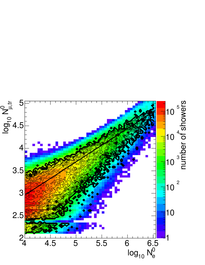
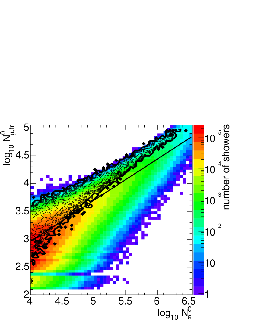
Figure 1: Number of muons versus number of electrons ($\log_{10}N_{\mu,tr}^{0}$ vs. $\log_{10}N_{e}^{0}$) of showers measured with KASCADE (shaded area). Simulated air showers induced by primary protons (left-hand side) or iron nuclei (right-hand side) are superimposed (contour lines). The straight lines in both figures indicate the separation between light and heavy primaries according to equation 4.

To evaluate the dependence of a possible Rayleigh amplitude on primary energy and mass, the data set is divided by a simple cut in the $\log_{10}N_{\mu,tr}$-$\log_{10}N_{e}$ plane into two sets. Simulation studies show, that showers initiated by light primary particles are predominately electron rich while those from heavy primaries are electron poor (Antoni et al., 2002). The extensive air showers are simulated utilising the CORSIKA package (Heck et al., 1998). The QGSJet-model (Kalmykov, Ostapchenko, & Pavlov, 1997) is used for hadronic interactions above $E_{Lab}>80$ GeV, GHEISHA (Fesefeldt, 1985) for interactions below this energy. The electromagnetic cascades are simulated by EGS4 (Nelson, Hirayama, & Rogers, 1985). The shower simulation is followed by a detector simulation based on GEANT (GEANT, 1993). A power law with constant spectral index of $\gamma=-2$ is used in the simulations. Figure 1 shows the distribution of muon number versus electron number ($\log_{10}N_{\mu,tr}^{0}$-$\log_{10}N_{e}^{0}$) of showers measured with KASCADE and from the mentioned simulations of proton- and iron-induced showers. There are several reasons for the differences between the measured and the simulated distributions. The chemical composition of cosmic rays consists of more than two components, the slope of the energy spectrum of the cosmic rays is different in the simulations and the number of measured showers exceeds by far the number of simulated showers.

A separation between light and heavy primaries can be expressed by the following ratio:

$$\log_{10}N_{\mu,tr}^{0}/\log_{10}N_{e}^{0}=0.74$$ (4)

The electron number $N_{e}$ and the truncated muon number $N_{\mu,tr}$ are zenith angle corrected to $\Theta=0$^∘ using the attenuation law:

$$N_{e}^{0} = N_{e}\cdot\exp{\left(X_{0}/\Lambda_{e}(\mathrm{sec}\Theta-1)\right)}$$ (5)

$$N_{\mu,tr}^{0} = N_{\mu,tr}\cdot\exp{\left(X_{0}/\Lambda_{\mu,tr}(\mathrm{sec}\Theta-1)\right)}$$ (6)

with the attenuation lengths $\Lambda_{N_{e}}=175$ g/cm² and $\Lambda_{N_{\mu,tr}}=823$ g/cm² (Antoni et al., 2003b).

This separation neglects the large fluctuations, especially of proton initiated showers. It also neglects the very different relative abundances of light to heavy primaries in cosmic rays.

5 Correction for atmospheric ground pressure and temperature

The influence of the atmospheric ground pressure $P$ and temperature $T$ on the rate of extensive air showers at ground is taken into account by a second order polynomial with additional time dependent corrections $\Delta R_{i}$ for $i$ different configurations of the detector system (e.g. with slightly different high-voltages of the detectors):

$$R(P,T,i)=R_{0} + \Delta R_{i}$$ (7)

$$+ p_{1}(P-P_{0})+p_{2}(P-P_{0})^{2}$$

$$+ p_{3}(T-T_{0})+p_{4}(T-T_{0})^{2}$$

$$+ p_{5}(P-P_{0})(T-T_{0})$$

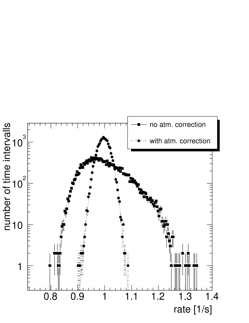
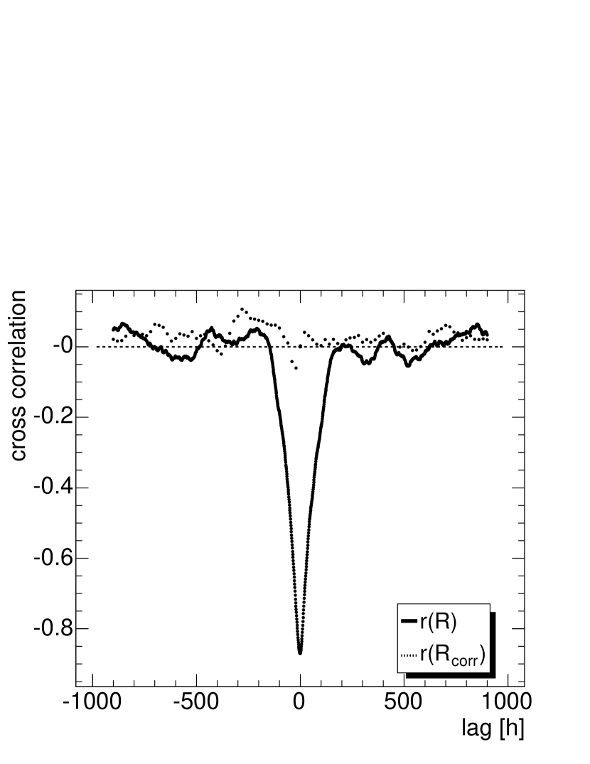
Figure 2: Left: Distribution of rates with and without correction for atmospheric ground pressure and temperature. A fit by a Gaussian function is shown by the line. Right: Cross correlation between hourly shower rate and atmospheric ground pressure with ($r(R_{corr})$) and without atmospheric correction ($r(R)$).

The detector parameters are constant during each of the $i$ time intervals. $R_{0}=0.966$ s^-1, $P_{0}=1002.95$ hPa , $T_{0}=9.7$^∘C  are the long-time mean values of rate, ground pressure, and temperature. All parameters $p_{1,2,3,4,5}$ and $\Delta R_{i}$ are estimated by a fit to the time dependent rates for the whole interval of four years and result in: $p_{1}=(-7.21\pm 0.0016)\cdot 10^{-3}$, $p_{2}=(-3.00\pm 0.13)\cdot 10^{-5}$, $p_{3}=(-3.64\pm 0.0023)\cdot 10^{-3}$, $p_{4}=(-3.19\pm 0.22)\cdot 10^{-5}$, and $p_{5}=(-3.76\pm 0.253)\cdot 10^{-5}$ in units of hPa, ^∘C, and seconds. The values for the $\Delta R_{i}$ are between $-2\times 10^{-2}$ and $2\times 10^{-2}$ s^-1. The correction itself is done for time intervals of 1795 s by subtracting or adding the necessary number of events calculated by Equation 7. Events are chosen randomly from the half-hour intervals to lower the number of showers. The events, which have to be added for this correction are chosen randomly from the set of showers of the same sidereal day. The quality of the correction can be estimated from Figure 2. The left figure shows the event rate distributions before and after the corrections. The uncorrected rates reflect the asymmetric distribution of the atmospheric ground pressure. The distribution of corrected rates is compatible with a Gaussian distribution, which is expected from remaining statistical fluctuations of the event rate. The right figure shows the cross correlation between rate and ground pressure. The very strong correlation $r(R)$ visible for the uncorrected rates vanishes after the correction ($r(R_{corr})$) with Equation 7.

6 Results

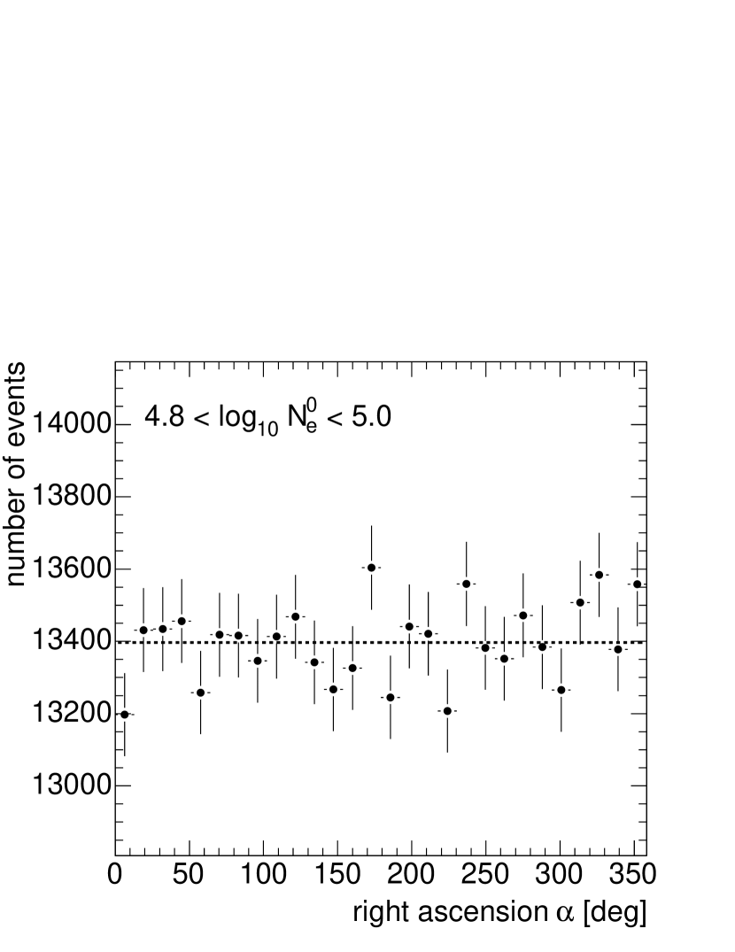
Figure 3: Example of a right ascension distribution after correction for atmospheric ground pressure and temperature in the stated electron number interval. The dashed line reflects the mean number of events.

An example for the right ascension distributions of showers after atmospheric correction for electron numbers in the interval $4.8<\log_{10}N_{e}^{0}<5$ is shown in Figure 3. The Rayleigh amplitudes $A$ of the right ascension distributions for electron numbers in the range from $\log_{10}N_{e}^{0}=4$ to $\log_{10}N_{e}^{0}=6.6$ are calculated according to Equation 1. The lower electron number limit is the efficiency threshold of the KASCADE detector field. As mentioned in section 3, full efficiency is required in order to minimize effects of the threshold to the amplitudes. The upper electron number limit at $\log_{10}N_{e}^{0}=6.6$ is determined by the small number of events ($\approx 1000$) in this electron number interval.

The showers are sorted in intervals of electron number $\log_{10}N_{e}^{0}$ and not in intervals of truncated muon number $\log_{10}N_{\mu,tr}^{0}$, although the latter one is a better estimator for primary energy and less dependent on the mass of the primary particle. The trigger threshold of the detector field is mainly determined by the number of electrons. The usage of $N_{\mu,tr}^{0}$ combined with the requirement of full detection efficency would shift the lower energy threshold of this analysis to energies above $4\times 10^{15}$ eV.

Figure 4 (left-hand side) shows the resulting Rayleigh amplitudes. The lines indicate the confidence levels for Rayleigh amplitudes with probabilities $1-P(>A)$ of 68/95/99 % respectively. Assuming a power law with spectral index $\gamma$ for the form of the electron size spectrum, the confidence levels are as well power laws with spectral indices of $-\gamma/2$ (see Equation 3). The confidence levels are only a function of the number of events used in the analysis. The increase of the confidence levels with electron number reflects therefore by no means an increase of anisotropy. Amplitudes which are below the lines indicating the confidence levels can be treated as fluctuations and are of no physical meaning. All calculated amplitudes are well below the 95% line. The fluctuation probability $P(>A)$ of each Rayleigh amplitude is shown in Figure 4 (right-hand side). The probabilities are all above 5% . There are no hints for nonzero Rayleigh amplitudes within the statistical limits.

The results of the two subsets of data containing electron-rich and electron-poor showers are shown in Figure 5. No correction for ground pressure $P$ and temperature $T$ is applied in this case. The variations of $P$ and $T$ alter beside the detection rate also the number of electrons and muons in a shower and therefore the effect of the separation line (Equation 4) between electron-poor and electron-rich showers. A further correction would require detailed information about the influence of atmospheric variations on $N_{e}$ and $N_{\mu,tr}$, which is beyond the scope of this analysis. Only a detection of significant amplitudes would require such further steps. As can be seen from Figure 5, no anisotropy can be deduced from the calculated amplitudes and fluctuation probabilities. The most prominent amplitude at $5<\log_{10}N_{e}^{0}<5.2$ has a significance of $\sigma=2.2$. The intersection of the confidence levels of electron poor and rich showers is due to the increasing fraction of heavy primary cosmic rays with increasing primary energy in the region of the knee (Antoni et al., 2002).

Additionally to the results presented in Figures 4 and 5, an analysis of the data set with different definitions of the electron number intervals and for showers above the knee sorted by truncated muon numbers yielded the same result of no significant amplitudes.

Figure 6 shows the upper limits on the large scale anisotropy derived in this analysis in context with results from other experiments and predictions from the model of Candia, Mollerach, & Roulet (2003). The primary energies of the extensive air showers measured by KASCADE are determined by a linear transformation of the particle numbers $\log_{10}N_{e}^{0}$ and $\log_{10}N_{\mu,tr}^{0}$. The transformation matrix is determined from CORSIKA simulations using the hadronic interaction models QGSJET and GHEISHA. The uncertainty of this simplified primary energy determination is about 20%. The figure shows that the KASCADE upper limits are in the range of the reported results from other experiments. The EAS-TOP experiment reported somewhat lower limits in the energy range below $2\times 10^{15}$ eV. The relatively large amplitudes published by the Akeno experiment are difficult to reconcile with the results of this analysis. The model calculations, which dependent of course on several parameters like the source distribution or the strength and structure of the galactic magnetic field, yield amplitudes in the range of $3\times 10^{-4}$ to $2\times 10^{-3}$ in the energy range of KASCADE. This is about a factor of 4-10 lower than the upper limits derived in this analysis. The contribution from anisotropy measurements towards a solution of the enigma of the knee are therefore still small. A significant observation of the anisotropy of separate cosmic ray components around and above the knee requires much larger data sets compared to the presently available.

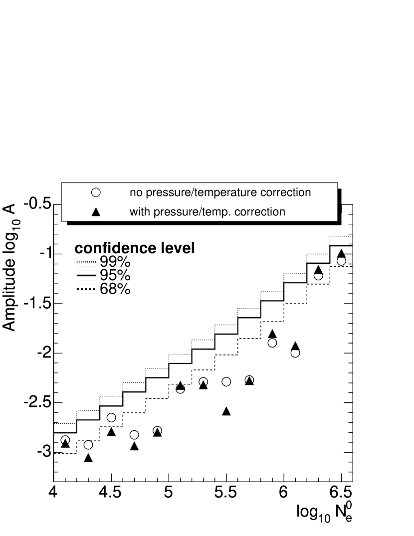
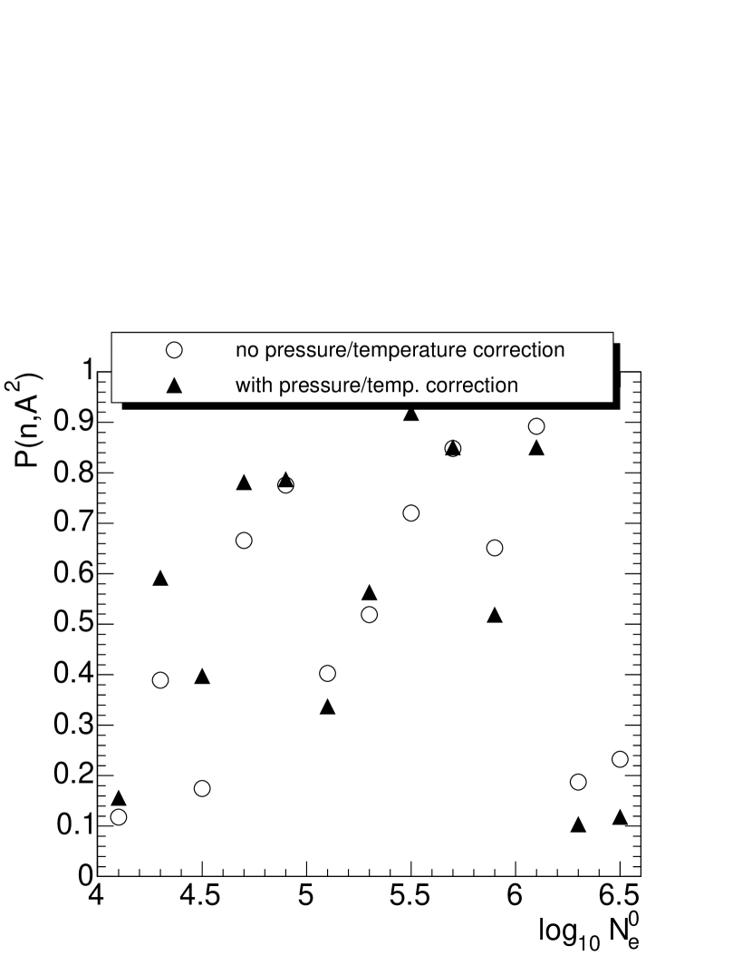
Figure 4: Result from the Rayleigh analysis for showers without and with correction for atmospheric ground pressure and temperature. Left-hand side: Rayleigh amplitude $A$ vs. electron number $\log_{10}N_{e}^{0}$. Right-hand side: Probability $P(n,A^{2})$ that the amplitudes plotted in the left figure are fluctuations from underlying uniform distributions.

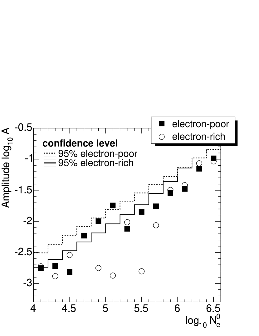
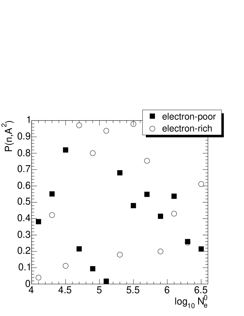
Figure 5: Result from the Rayleigh analysis for data sets of predominately light and heavy primaries. Left-hand side: Rayleigh amplitude $A$ vs. electron number $\log_{10}N_{e}^{0}$. Right-hand side: Probability $P(n,A^{2})$ that the amplitudes in the left figure are fluctuations from underlying uniform distributions.

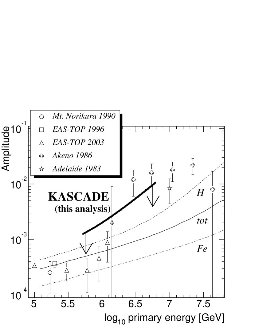
Figure 6: KASCADE upper limits (95%) of Rayleigh amplitudes $A$ vs. primary energy (bold line) compared to reported results from literature (Nagashima et al., 1990; Aglietta et al., 1996, 2003; Kifune et al., 1986; Gerhardy & Clay, 1983). Model predictions from Candia, Mollerach, & Roulet (2003) for the total anisotropy and for anisotropies of the proton and iron component are shown as well (thin lines).

References

- Aglietta et al. (1996) Aglietta, M. et al. (The EAS-TOP Collaboration) 1996, ApJ, 470, 501
- Aglietta et al. (2003) Aglietta, M. et al. (The EAS-TOP Collaboration) 2003, Proc. of 28th ICRC, Tsukuba, vol.4, p.183
- Antoni et al. (2002) Antoni, T. et al. (KASCADE collaboration) 2002, Astropart. Phys., 16, 373
- T. Antoni et al. (2003a) Antoni, T. et al. (KASCADE Collaboration) 2003a, Nucl. Instr. and Meth., A, 513, 490
- Antoni et al. (2003b) Antoni, T. et al. (KASCADE collaboration) 2003b, Astropart. Phys., 19, 703
- Candia, Mollerach, & Roulet (2003) Candia, J., Mollerach, S., & Roulet, E. 2003, Journal of Cosmology and Astropart. Phys, 5, 3
- GEANT (1993) CERN 1993, GEANT 3.21, Detector Description and Simulation Tool, CERN Program Library Long Writeup W5015, Application Software Group
- Clay, McDonough, & Smith (1997) Clay, R., McDonough, M.-A., & Smith, A. 1997, Proc. of 25th ICRC, Durban, vol.4, p.185
- Fesefeldt (1985) Fesefeldt, H. 1985, Report PITHA-85/02, RWTH Aachen
- Gerhardy & Clay (1983) Gerhardy, P. & Clay, R. 1983, J. Phys. G, 9, 1279
- Heck et al. (1998) Heck, P. et al. 1998 Report FZKA 6019, Forschungszentrum Karlsruhe
- Kalmykov, Ostapchenko, & Pavlov (1997) Kalmykov, N.N., Ostapchenko, S.S., & Pavlov, A.I. 1997, Nucl. Phys. B. (Proc. Suppl.), 52B 17
- Kifune et al. (1986) Kifune, T. et al. 1986, J. Phys. G, 12, 129
- Lagage & Cesarsky (1983) Lagage, P. & Cesarsky, C. 1983, A&A, 118, 223
- Mardia & Jupp (1999) Mardia, V. & Jupp, P. 1999, Directional statistics, John Wiley & Sons
- Nagashima et al. (1990) Nagashima, K. et al. 1990, Proc. of 21st ICRC, Adelaide, vol.3, p.180
- Nelson, Hirayama, & Rogers (1985) Nelson, W.R., Hirayama, H., & Rogers, D.W.O. 1985, Report SLAC 265, Stanford Linear Accelerator Centre