Ultra-High Energy Cosmic Rays from Quasar Remnants

Abstract

One of the models recently proposed to explain the origin of the ultra high energy cosmic rays assumes that these particles may be accelerated by the electromotive force around presently inactive quasar remnants. We study predictions for large and small scale ultra high energy cosmic ray arrival direction anisotropies in a scenario where the particles are injected with a mono-energetic spectrum by a discrete distribution of such sources. We find that known quasar remnants are typically distributed too anisotropically to explain the isotropic ultra high energy cosmic ray flux except in the unrealistic case where extragalactic magnetic fields of $\simeq 0.1\mu$G extend over many Mpc.

Keywords: uhc, blh, maf

FERMILAB-Pub-03/402-A, MADPH-03-1337

1 Introduction

Over the last few years the detection of several giant air showers, either through ground based detectors [1, 2] or fluorescence telescopes  [3, 4], have confirmed the arrival of ultra high energy cosmic-rays (UHECRs) with energies up to a few hundred EeV (1 EeV $\equiv 10^{18}\,$eV). Their existence poses a serious challenge and is currently subject of much theoretical research as well as experimental efforts (for recent reviews see [5, 6, 7]).

The problems encountered in trying to explain UHECRs in terms of “bottom-up” acceleration mechanisms have been well-documented in a number of studies (e.g., Refs. [8, 9, 10]). In summary, apart from energy draining interactions in the source, the maximal UHECR energy is limited by the product of the accelerator size and the strength of the magnetic field. According to this criterion it turns out that it is very hard to accelerate protons and heavy nuclei up to the observed energies, even for the most powerful astrophysical objects such as radio galaxies and active galactic nuclei.

In addition, nucleons above $\simeq 50\,$EeV suffer heavy energy losses due to photo-pion production on the cosmic microwave background (CMB) — the Greisen-Zatsepin-Kuzmin (GZK) effect [11] — which limits the distance to possible sources to less than $\simeq 100\,$Mpc [12]. Heavy nuclei at these energies are photo-disintegrated in the CMB within a few Mpc [13]. Unless the sources are strongly clustered in our local cosmic environment, a drop, often called the “GZK cut-off” in the spectrum above $\simeq 50\,$EeV is therefore expected [14], even if injection spectra extend to much higher energies. However, the existence of the latter is not established yet from the observations [15]. In fact, whereas a cut-off seems consistent with the few events above $10^{20}\,$eV recorded by the fluorescence detector HiRes [4], it is not compatible with the 8 events (also above $10^{20}\,$eV) measured by the AGASA ground array [2]. The solution of this problem may have to await the completion of the Pierre Auger project [16] which will combine the two complementary detection techniques adopted by the aforementioned experiments.

Adding to the problem, there are no obvious astronomical counterparts to the detected UHECR events within $\simeq 100\,$Mpc of the Earth [17, 9]. At the same time, no significant large-scale anisotropy has been observed in UHECR arrival directions above $\simeq 10^{18}\,$eV, whereas there are strong hints for small-scale clustering: The AGASA experiment has observed four doublets and one triplet within $2.5^{\circ}$ out of a total of 57 events detected above 40 EeV [2]. When combined with three other ground array experiments, these numbers increase to at least eight doublets and two triplets within $4^{\circ}$ [18]. This clustering has a chance probability of less than $1\%$ in the case of an isotropic distribution.

There are currently two possible explanations of these experimental findings. In the first one, which assumes negligible magnetic deflection, most of the sources would have to be at cosmological distances which would explain the absence of nearby counterparts and the apparent isotropy would indicate that many sources contribute to the observed flux, where a subset of specially powerful sources would explain the small-scale clustering [19]. This scenario predicts the confirmation of a GZK cutoff. The second scenario is more realistic and takes into account the likely existence of large scale intervening magnetic fields correlated with the large scale galaxy distribution. In this case magnetic deflection could be considerable even at the highest energies and the observed UHECR flux could be dominated by relatively few sources within about 100 Mpc. Here, large scale isotropy could be explained by considerable angular deflection leading to diffusion up to almost the highest energies and magnetic lensing [20] could contribute to the small scale clustering.

A possible way of explaining the origin of these particles is to assume a source population associated with quasar remnants currently inactive in the visible spectrum [21]. If these sources are sufficiently numerous, this would explain large scale isotropy, whereas a few nearby sources could explain the small scale clustering. In this scenario, UHECRs would be accelerated at the nuclei of those nearby dead quasars, whose underlying super-massive black holes are sufficiently spun-up to provide the necessary electromotive force. Hints of a possible correlation between some of these dormant quasars and the arrival direction of cosmic rays above $4\times 10^{19}\,$eV may support this scenario [22].

In the present study we perform numerical simulations in order to test a sample of candidate dead quasars as possible sources for the ultra high energy events. We first considered the case of an all-pervading turbulent magnetic field of 1nG strength, which corresponds to the primordial field necessary to explain galactic magnetic fields by adiabatic compression [23]. We also performed simulations with a relatively strong magnetic field of $0.1\mu$G, either following a pancake like structure mimicking the Local Supercluster, or homogenous up to the farthest sources. All these cases are consistent with Faraday rotation upper limits [24], although the strong field case may not be very realistic.

The paper is organised as follows: in Sec.II we outline the scenario underlying our numerical simulations which are briefly described in Sec.III. In Sec.IV we introduce the statistical quantities used for comparison with the data. In Sec.V we present our results and we conclude in Sec.VI.

2 The Quasar Remnant Scenario

Boldt and Ghosh [21] suggested that supermassive black holes, present in the center of normal galaxies [25], could be the principal sources of particles at the highest energies. As stressed in the introduction, the lack of observed counterparts to the highest energy events within an acceptable distance suggests the idea of sources currently inactive in the visible spectrum. These objects should be able to accelerate UHECRs and appear dormant at the same time. Quasars remnants or dormant AGNs (active in earlier phases), with underlying supermassive black holes, are among the astronomical objects which best satisfy these requirements. In this model the black holes were spun up to nearly their maximal spins during an earlier phase, when the dormant AGNs were active, and liberate their rotational energy in the form of UHE particles rather than in powerful jets.

The acceleration is due to the potential difference produced by magnetic field lines threading the event horizon of the supermassive black hole in rotation. The electromotive force generated by a rotating black hole of mass $M$, threaded by a magnetic field of strength $B$ extending on a range $R\approx R_{g}$ (gravitational radius $\equiv GM/c^{2}$) is given by [26]

$$emf\approx 9\times 10^{20}\left(a/M\right)B_{4}M_{9}\,\,{\rm volts}\,\,$$ (1)

where $a$ is the black hole specific angular momentum, $B_{4}\equiv B~{}/(10^{4}G)$ and $M_{9}\equiv M/(10^{9}M_{\odot})$. For a rapidly spinning hole, we can approximate $a/M\simeq 1$ which gives the maximal estimated energy.

Apart from the mass of the object, the only input to estimate the maximal energy achievable in a given supermassive black hole is the magnetic field which will depend on the mass accretion rate. By assuming pressure equilibrium between the magnetic field and the infalling matter we have [21]

$$B_{4}=1.33M_{9}^{-1}\dot{M}^{1/2}\,,$$ (2)

where $\dot{M}$ is the mass accretion rate in units of $M_{\odot}/yr$. From Eqs. 1 and 2 we obtain

$$emf\approx 1.2\times 10^{21}\dot{M}^{1/2}\,\,{\rm volts}\,.$$ (3)

In the present case, we consider protons as primary for which the energy loss dominant processes during the acceleration phase are due to pair production and photomeson production on ambient photons. We will neglect these energy losses at the source because an exceptional low accretion luminosity characterizes the supermassive black holes at the centers of nearby bright galaxies [27] making the mean free path for this interaction larger than $R_{g}$. The losses due to curvature radiation induced by the magnetic field are taken into acount as in Ref. [28]. Furthermore, as in [22], we assume the accretion rate onto the black hole to be about 10% of the bulge mass loss rate, $\dot{M}\simeq 0.1M_{12}^{B}$, with $M^{B}_{12}\equiv M_{bulge}/(10^{12}M_{\odot})$, and $M_{bulge}$ the bulge mass. The maximal proton energy expected is then given by

$$E_{\rm max} = 137(\dot{M})^{1/8}(M_{9})^{1/4}{\rm EeV}$$ (4)

$$\sim 104(M^{B}_{12})^{1/8}(M_{9})^{1/4}{\rm EeV}\,.$$

The list of sources we will use in our numerical simulations are given in Table 1 and is obtained by selecting from the table of massive dark objects in nearby galaxies given by Magorrian et al. [25, 29], Kormendy [30], and Marconi et al. [31] those which could accelerate particles beyond $4\times 10^{19}$ eV. We do not include NGC 4486 as from recent estimates of the spectral energy distribution at the core of this galaxy it is not possible to accelerate particles to the highest energy by the compact dynamo considered here [21] (second reference). Injection rates of individual sources are represented by a weight factor given by the mass accretion rate in units of $M_{\odot}/yr$ divided by the maximal energy in units of EeV. These weight factors are shown in the last column of Table 1.

Table 1: The list of sources used in our simulations. Here, $D$ is the distance to the source in Mpc, $M_{9}\equiv M/(10^{9}M_{\odot})$, $M^{B}_{12}=M_{\rm bulge}/(10^{12}M_{\odot})$, $E_{max}^{19}\equiv E_{max}/(10^{19}{\rm eV})$, $\alpha$ and $\delta$ are the equatorial coordinates and WF is the weight factor $\times 10^{4}$.

• 	Galaxy	D	$M_{9}$	$M^{B}_{12}$	$E_{\rm max}^{19}$	${\alpha}^{\circ}$	${\delta}^{\circ}$	WF
  1	NGC821	24.1	0.19	0.12	5.33	31.42	10.76	2.3
  2	NGC1399	17.9	5.2	0.32	13.7	54.14	-35.61	2.3
  3	IC1459	29.2	1.5	0.66	11.0	343.60	-36.29	6.0
  4	NGC1600	50.2	11.6	1.29	19.9	67.30	-5.19	6.5
  5	NGC2300	34.0	2.7	0.39	12.0	108.94	85.81	3.3
  6	NGC2832	90.2	11.4	0.98	19.1	139.18	33.96	5.1
  7	NGC3115	9.7	0.35	0.14	6.3	150.69	-7.48	2.2
  8	NGC3245	20.9	0.21	0.04	4.7	156.13	28.76	0.82
  9	NGC3379	10.6	0.39	0.076	6.0	161.30	12.85	1.2
  10	NGC3608	22.9	0.25	0.11	5.6	168.59	18.42	1.9
  11	NGC4168	36.4	1.19	0.27	9.3	182.43	13.48	2.9
  12	NGC4261	31.6	0.52	0.04	8.0	184.21	8.02	5.6
  13	NGC4278	17.5	1.56	0.14	9.1	184.41	29.56	1.5
  14	NGC4291	26.2	1.86	0.12	9.3	184.52	75.65	1.3
  15	NGC4342	11.4	0.22	0.01	4.0	185.28	7.32	0.25
  16	NGC4374	18.4	1.60	0.54	10.8	185.63	13.16	4.9
  17	NGC4459	16.1	0.07	0.36	4.7	186.62	14.25	7.6
  18	NGC4472	15.3	2.7	0.84	12.9	186.82	8.27	6.5
  19	NGC4473	15.8	0.34	0.09	6.0	186.82	13.71	1.6
  20	NGC4486b	16.1	0.92	0.003	4.9	186.99	12.77	0.06
  21	NGC4552	15.3	0.47	0.14	6.8	188.28	12.83	2.1
  22	NGC4564	15.3	0.25	0.04	5.0	188.48	11.71	0.88
  23	NGC4594	9.8	0.69	0.29	8.1	189.33	-11.33	3.6
  24	NGC4621	15.3	0.28	0.19	6.1	189.88	11.92	3.1
  25	NGC4636	15.3	0.23	0.32	6.2	190.07	2.96	5.2
  26	NGC4649	16.8	3.9	0.55	13.6	190.28	11.83	4.0
  27	NGC4660	15.3	0.28	0.01	4.4	190.50	11.46	0.31
  28	NGC4697	11.7	0.17	0.20	5.5	191.50	-5.53	3.6
  29	NGC4874	93.3	20.8	2.08	24.4	194.30	28.23	8.5
  30	NGC4889	93.3	26.8	1.28	24.5	194.43	28.24	5.2
  31	NGC5128	4.2	0.24	0.06	5.1	200.63	-43.76	1.1
  32	NGC5252	96.8	1.0	0.24	8.7	203.93	4.80	2.7
  33	NGC5845	25.9	0.24	0.02	4.4	225.87	1.83	0.43
  34	NGC6166	112.5	28.4	1.66	25.7	246.73	39.66	6.5
  35	NGC6251	107.0	0.61	0.67	8.8	249.49	82.64	7.6
  36	NGC7052	71.4	0.40	0.60	7.8	319.09	26.23	7.7
  37	NGC7768	103.1	9.1	0.89	17.9	357.11	26.87	5.0

3 Numerical simulations

The list of sources given in Table 1 has been implemented into the numerical code for UHECR propagation in extragalactic magnetic fields used in earlier studies, see Refs. [32, 33] for details.

For each configuration many nucleon trajectories originating from the sources were computed numerically by solving the equation of motion for the Lorentz force and checking for pion production every fraction of a Mpc according to the total interaction rate with the CMB. In case of an interaction, secondary energies were randomly selected according to the differential cross section. Pair production by protons is treated as a continuous energy loss process.

Each trajectory is abandoned if the particle reaches a distance from the observer twice bigger than the distance to the farthest source, i.e. 230 Mpc, or if the propagation time exceeds 10 Gyr.

A detection event was registered and its arrival direction and energy recorded each time the trajectory of the propagating particle crossed a sphere of radius 1 Mpc around the observer. For each configuration this was done until 5000 events where registered. For each detected event, we register also the source by which it has been emitted.

We assume a mono-energetic injection spectrum at the source: all particles coming from a source are emitted with the maximal energy of acceleration for that source as given in Table 1. We take into account the individual source power by including the weight factor in the last column of Table 1.

We assume a random turbulent magnetic field with power spectrum $<B(k)^{2}>\propto k^{n_{B}}$ for $(2\pi/1{\rm Mpc})<k<(2\pi/0.01{\rm Mpc})$ and $\langle B(k)^{2}\rangle=0$ otherwise. The magnetic field modes are computed on a linear grid in momentum space and are Fourier transformed onto the corresponding grid in location space. The r.m.s. strength $B$ is given by $B^{2}=\int_{0}^{\infty}\,dk\,k^{2}\left\langle B^{2}(k)\right\rangle$. We use $n_{B}=-11/3$, corresponding to Kolmogorov turbulence.

This turbulent spectrum is applied to three different cases: the first case is an all-pervading relatively weak magnetic field $\simeq 1\,$nG. For the case of a relatively strong magnetic field we performed two simulations: in the first one the field follows a rough representation of the Local Supercluster, a pancake profile with scale height of 12 Mpc and scale length of 25 Mpc; the center of the profile as at the Virgo cluster, 20 Mpc from the observer who is located in the plane of the pancake. The maximal field strength at the Virgo cluster equals 0.1$\mu$G. Its strength at the observer is then $B=0.5\times 10^{-7}\,$Gauss. In the second simulation we consider an all-pervading field of strength $B=0.1\,\mu$G.

4 Multi-poles and Autocorrelation function

For each simulated sky distribution typically 1000 mock data sets consisting of $N_{\rm obs}$ observed events were selected randomly and multiplied with the solid-angle dependent exposure function. For each such mock data set or for the real data set we then obtained estimators for the spherical harmonic coefficients $C(l)$ and the autocorrelation function $N(\theta)$. The estimator for $C(l)$ is defined as

$$C(l)=\frac{1}{2l+1}\frac{1}{{\cal N}^{2}}\sum_{m=-l}^{l}\left(\sum_{i=1}^{N_{\rm obs}}\frac{1}{\omega_{i}}Y_{lm}(u^{i})\right)^{2}\,,$$ (5)

where $\omega_{i}$ is the total experimental exposure at arrival direction $u^{i}$, ${\cal N}=\sum_{i=1}^{N_{\rm obs}}1/\omega_{i}$ is the sum of the weights $1/\omega_{i}$, and $Y_{lm}(u^{i})$ is the real-valued spherical harmonics function taken at direction $u^{i}$. For a detector at a single site we use the following parameterization:

$$\omega(\delta)\propto\cos a_{0}\cos\delta\sin\alpha_{m}+\alpha_{m}\sin a_{0}\sin\delta\,,$$ (6)

where $a_{0}$ is the latitude of the detector and $\alpha_{m}$ is zero for $\xi>1$, $\pi$ for $\xi<-1$, and $\cos^{-1}(\xi)$ otherwise, where $\xi\equiv(\cos\theta_{m}-\sin a_{0}\sin\delta)/[\cos a_{0}\cos\delta]$.

In Table 2 we give a list of the experimental features for the three experiments used in the next section. In order to have maximal sky coverage for the large scale multi-poles, we included data from the SUGAR array which operated from January 1968 to February 1979 in Australia at a latitude of $30.5^{\circ}$ South and $149^{\circ}38^{\prime}$ East [34].

Table 2: Experiments considered in the present study. Here, ${\rm Res.}^{40}$ is the angular resolution for energies above $40{\rm EeV}$, $a_{0}^{N(S)}$ is the latitude North (South) of the experiment and the angle $\theta_{m}$ is the maximal zenith angle out to which the detector is fully efficient.

• Exp	${\rm Res.}^{40}$	$a_{0}^{N}$	$a_{0}^{S}$	$\theta_{m}$
  AGASA	$1.6^{\circ}$	$+35.5^{\circ}$		$45^{\circ}$
  SUGAR	$10^{\circ}$		$-30.5^{\circ}$	$55^{\circ}$
  AUGER	$1.^{\circ}$	$+35^{\circ}$	$-39^{\circ}$	$60^{\circ}$

The estimator for $N(\theta)$ is defined as

$$N(\theta)=\frac{C}{S(\theta)}\sum_{j\neq i}\left\{\begin{array}[]{ll}1&\mbox{if $\theta_{ij}$ is in same bin as $\theta$}\\ 0&\mbox{otherwise}\end{array}\right\}\,,$$ (7)

where $S(\theta)$ is the solid angle size of the corresponding bin and $C=\Omega_{e}/(N_{\rm obs}(N_{\rm obs}-1))$, with $\Omega_{e}$ denoting the solid angle of the sky region where the experiment has non-vanishing exposure. In both cases for each $l$ we plot the average over all trials and realizations as well as two error bars. The smaller error bar (shown to the left of the average) is the statistical error, i.e. the fluctuations due to the finite number $N_{\rm obs}$ of observed events, averaged over all realizations, while the larger error bar (shown to the right of the average) is the “total error”, i.e. the statistical error plus the cosmic variance, in other words, the fluctuations due to the finite number of events and the variation between different realizations of the magnetic field.

In the figures shown in Sec.V, the histogram represents the data and the solid line represents the analytical prediction for an isotropic distribution in the case of future predictions. Given a set of observed and simulated events we define

$$\chi_{n}\equiv\sum_{i}\left(\frac{S_{i,{\rm data}}-\overline{S}_{i,{\rm simu}}}{\Delta S_{i,{\rm simu}}}\right)^{n}\,,$$ (8)

where $S_{i,{\rm data}}$ refers to $C_{l}$ and $N(\theta)$ defined above, obtained from the real data, and $\overline{S}_{i,{\rm simu}}$ and $\Delta S_{i,{\rm simu}}$ are the average and standard deviations of these quantities obtained from the simulated data sets. This measure of deviation from the average prediction is used to obtain an overall likelihood ${\cal L}$ for the consistency of a given theoretical model with an observed data set by counting the fraction of simulated data sets with $\chi_{n}$ larger than the one for the real data. The likelihoods are computed for n=4 in Eq. 8.

5 Results

In the following we compare the results obtained for the simulated UHECR propagation scenarios described above with the observational results. As discussed in the previous section, the comparison is based on the statistical properties of the simulated and observed events, expressed in terms of the angular power spectrum and the autocorrelation function of the UHECR arrival distributions.

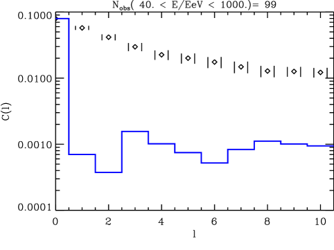
Figure 1: The angular power spectrum $C(l)$ as a function of multi-pole $l$, obtained for the AGASA+SUGAR exposure function, for ${\rm N}_{\rm obs}$=99 events observed above 40 EeV, sampled from 15 simulated configurations with $B=1\,$nG. The diamonds indicate the realization averages, and the left and right error bars represent the statistical and total (including cosmic variance due to different realizations) error, see text. The histogram represents the AGASA+SUGAR data. The total likelihood for this fit is $\ll 10^{-3}$.

To estimate the true power spectrum from Eq. (5) requires data with full sky coverage and therefore at least two detector sites such as foreseen for the Pierre Auger experiment. We therefore combine data from the AGASA and SUGAR experiments which had comparable exposure in the northern and southern hemisphere, respectively. The data set is made of 99 events: the 50 from AGASA (excluding 7 events observed by Akeno) and the 49 from Sugar above $4\times 10^{19}$eV. Usually care has to be taken in combining data from two experiments with significantly different angular resolution, see Table 2. This is possible only for multi-poles $l\leq 10$ which are not sensitive to scales $\leq 10^{\circ}$, as pointed out in [35].

In Fig.1 we compare with the combined AGASA+SUGAR data the angular power spectrum predicted by simulations for a scenario with all-pervading fields of r.m.s. strength $B=1\,$nG. The large predicted anisotropy is due to the fact that the sources follow the supergalactic plane and that UHECRs do not diffuse on the scale of the distance to the dominant, relatively close sources, since their Larmor radius $r_{L}\simeq 110(E/10^{20}eV)(B/10^{-9}G)^{-1}\,$Mpc. In addition, the distribution of events is concentrated around the directions to a few close sources which give the principal contribution to the detected flux. This can be understood by considering, in Fig.2, the number of events detected from source “$i$” in a given range of energy $n_{i}(E_{1}<E<E_{2})$, normalized to the total number of events detected from all sources in the same energy range, $n_{\rm tot}(E_{1}<E<E_{2})$, for this weak field case. The labels on the x axis correspond to the distances of sources in Mpc whereas at the top of each bin we mark the maximal acceleration energy of that source. Almost all particles are detected in the range between 40-100 EeV, whereas only $12\%$ of the total 75000 particles are detected outside this interval. The corresponding histogram also shows that only the sources in the list within 20 Mpc from Earth give a significant contribution. In case of negligible deflection we expect that clusters just reflect the point-like sources; if the number of observed events $N_{\rm obs}$ is larger than the number of contributing sources, as in the present scenario, each source contributes on average more than one event and strong clustering is expected. In addition, most of the closest sources are within an angular distance less than $5^{\circ}$ from each other. This implies that most of the events come from the same direction, and leads to a predicted autocorrelation function which at scales of a few degrees is about 30 times the value obtained from AGASA data.

The contribution of sources injecting above 40 EeV is strongly suppressed below this energy by two effects: the closest sources can give a contribution at low energies only when their maximal acceleration energy is close to 40 EeV, but they are sparse in the list considered here; the source NGC 4342 at 11.4 Mpc with ${\rm E}_{\rm max}=40\,$EeV is responsible for the first peak in the distribution below 40 EeV in Fig. 2. The farthest sources in contrast do not contribute below $\simeq 40\,$EeV because their maximal acceleration energy is sufficient to keep the energy of the particles above 40 EeV in the non diffusive regime. Fig. 2 shows that the contribution from the farthest sources is actually negligible at all energies, due to suppression by a factor proportional to “weight factor$/D^{2}$”, where $D$ is the distance to the source.

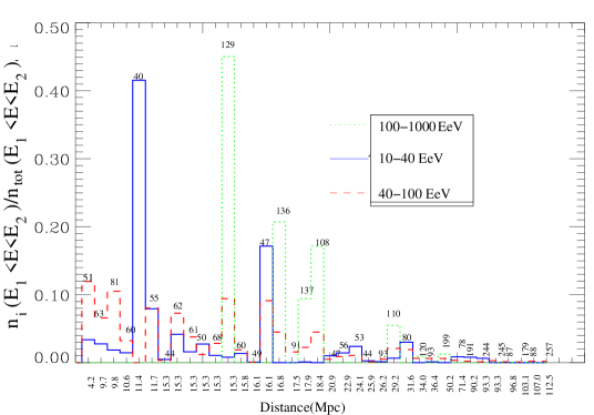
Figure 2: The number of detected events per source in a given range of energy, normalized to the total number of events detected in the same range of energy, averaged over 15 realizations, for the simulation with $B=1\,$nG. The x axis represents the distance corresponding to each source in Mpc. At the top of each histogram the maximal acceleration energy per source is shown. The solid line corresponds to the range (10-40) EeV, the dashed one to the range (40-100) EeV, and the pointed one to the range (100-1000) EeV.

So far we have found that the list of sources, as given in Table 1, cannot reproduce current data. If typical deflections are small, consistency with the data requires source distributions that are more homogeneously distributed than our sample in Table 1. If at least some of the sources in our list contribute significantly to the total flux, we would still expect a significant correlation between the arrival direction of the events and the positions of some of the objects in our list.

Following the same approach as in Ref. [28] we made a simple estimate of the positional coincidence between the sources in Table 1 and the UHECR events observed by AGASA with energy above $4\times 10^{19}$ eV. We calculate the number of real coincidences in circles centered on the position of a given source. For a circle radius of $4.8^{\circ}$, corresponding to a $3\sigma$ error box in angular resolution, coincidences with the AGASA data were only found for two relatively far sources, namely NGC4874 and NGC4889, and the source NGC 821 at 24 Mpc, which contribute negligibly to the flux, see Fig. 2. The source with the largest individual contribution (NGC5128) would predict $\simeq 6$ events in the range between 40 and 100 EeV, with a Poisson probability for no coincidence of about 0.1%. This implies that either deflection has to be significant and/or a considerable part of the observed flux is due to sources not in our list. We note in this context that hints of UHECR arrival direction correlations with another list of quasar remnants have been reported in Ref. [22].

We now investigate whether stronger magnetic fields, by providing larger angular deflection, might provide a better match to the observational data for this same source distribution. We performed simulations in turbulent magnetic fields following the profile of a sheet centered at 20 Mpc from Earth with strength $0.1\mu$G at the center of the sheet. We recall that infinitely extended profiles are consistent with Faraday rotation limits for fields up to fractions of a micro Gauss [24]. In Figs. 3 and 4 we show the autocorrelation function and angular distribution, respectively, above $4\times 10^{19}\,$eV, predicted by a simulation performed with fields following a pancake profile of scale length 25 Mpc and scale height 12 Mpc. The predictions are still not consistent with the data for our set of sources. Scenarios for pancake scale heights up to $\simeq 25\,$Mpc lead to similar results.

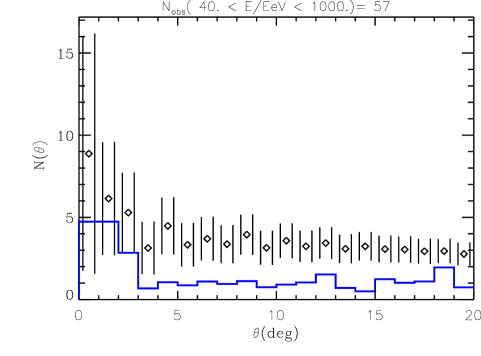
Figure 3: The angular correlation function $N(\theta)$, eq. (7), as a function of the angular distance $\theta$, using a bin size of $\Delta\theta=1^{\circ}$, obtained for the AGASA exposure function, for ${\rm N}_{obs}$=57 events observed above 40 EeV, sampled from 10 simulated realizations for a magnetic field following a pancake profile of scale length 25 Mpc and scale height 12 Mpc with $B=0.1\mu$G at the center. The diamonds indicate the realization averages, and the left and right error bars represent the statistical and total (including cosmic variance due to different realizations) errors respectively; see text for explanations. The histogram represents the AGASA data. The total likelihood for this fit is 0.01.

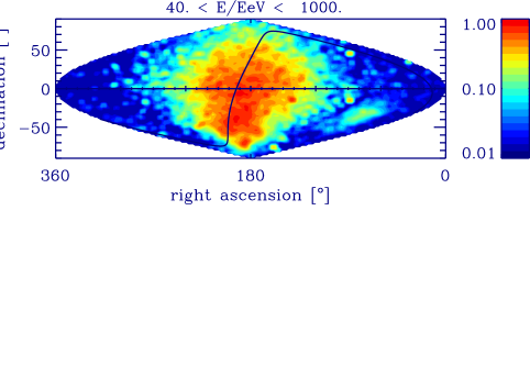
Figure 4: Angular distribution in equatorial coordinates on the celestial sphere for the same scenario as in Fig. 3. The solid line marks the supergalactic plane. The grey scale represents the integral flux per solid angle. The pixel size is $1^{\circ}$; the image has been convolved to an angular resolution of 1.6^∘ corresponding to AGASA.

In the scenario discussed above, the profile of the magnetic field in the sheet is such that the field is stronger in the middle plane than on the boundaries of the sheet. In Figs. 5 and 6 we show the angular distribution and the autocorrelation function, respectively, in the case where a magnetic field is distributed homogeneously rather than following a profile, although this is not a realistic scenario for our structured universe. As a result, when the effects of the boundary are absent, the predictions are more consistent with the data and the final distribution appears more isotropic.

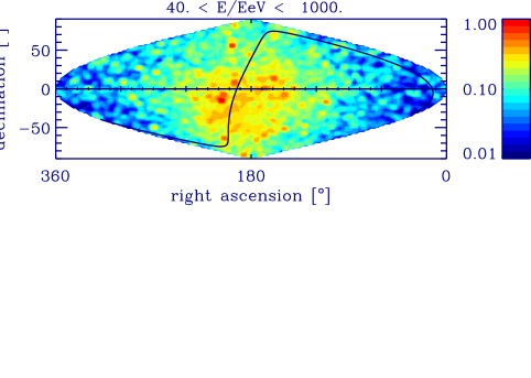
Figure 5: Same as Fig.4, but for a magnetic field $B=0.1\mu$G distributed homogeneously.

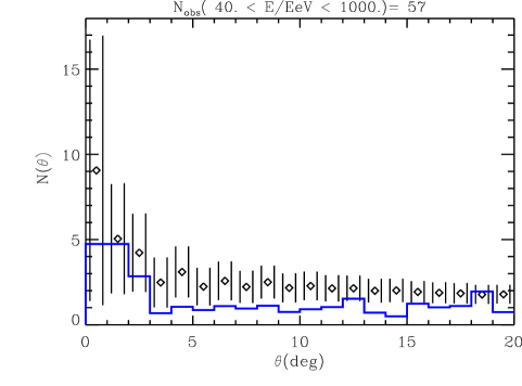
Figure 6: Same as Fig. 3, but for homogeneous field of $0.1\mu$G. The total likelihood for this fit is 0.18.

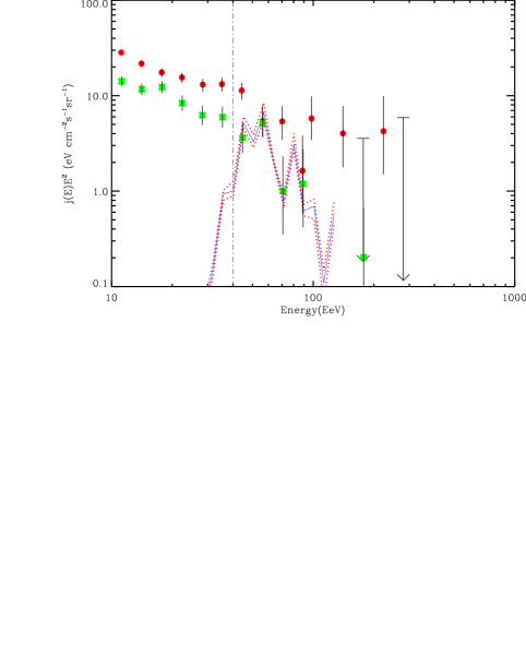
Figure 7: The realization averaged energy spectra corresponding to Figs. 5,6. The solid line represents the spectrum that would have been detected by AGASA, using the exposure Eq. (6). The dotted lines are the fluctuations due to the different magnetic field realizations and the one sigma error bars indicate the AGASA data (full dot) and HiRes data (asterisk).

In Fig. 7 we compare the spectrum predicted for this scenario with the AGASA and HiRes data. At the highest energies the cut-off is simply due to the fact that the maximal injection energy is 257 EeV, whereas we did not attempt to explain the flux below $\sim 40\,$EeV as we only included sources accelerating beyond this energy in our simulations. Less massive quasar remnants could well significantly contribute in this energy range as well.

The spectrum has been normalized to optimally fit the AGASA data which requires an average UHECR emission power of $\sim 10^{41}$erg/s for the nearby sources. At the same time the maximum power that can be extracted from a Kerr black hole is given by $L_{BH}\simeq 10^{40}(a/M)^{2}M_{6}^{2}B_{4}^{2}\,\,{\rm erg}\,\,{\rm s}^{-1}$ [36]. Using Eq. (2), the definition of $\dot{M}$ and the approximation $(a/M)\simeq 1$, as before, we parametrize the UHECR power as

$$L_{CR}\simeq\alpha_{CR}(0.17)10^{46}{M}_{12}^{B}\,\,{\rm erg}\,{\rm s}^{-1}\,,$$ (9)

where $\alpha_{CR}$ is the fraction of the power emitted as UHECRs. Comparing these two numbers and using typical bulge masses given in Table 1 for the closest sources implies a required UHECR injection efficiency of about $1\%$ of the accretion rate.

The spectrum in Fig. 7 shows no very pronounced GZK cut-off. This provides an important test for future experiments, especially the Pierre Auger project, which will be able to eventually confirm or falsify the presence of a GZK cut-off in the spectrum. If this cut-off is not observed, the quasar remnant scenario for UHECR origin here investigated could be promising good possibility but with a larger sample of sources such as to reproduce the observed isotropy at large scale. Future projects may provide sufficient statistics to probe the wiggles seen in Fig. 7 predicted by the monoenergetic injection.

In Fig.8 we shown the angular power spectrum for the exposure of the Pierre Auger experiment with full sky coverage, assuming 1500 events observed above 40 EeV, for the case of an all-pervading $0.1\,\mu$G field. For the exposure function we add Eq. 6 for two sites located at $a_{0}=-35^{\circ}$ and at $a_{0}=39^{\circ}$. The solid line represents the analytical prediction for a fully isotropic distribution, predicting $C_{l}\simeq(4\pi N_{\rm obs})^{-1}$. This scenario predicts an anisotropy that should be easily detectable by the Pierre Auger experiment.

Figure 8: The angular power spectrum $C(l)$ as a function of multi-pole $l$, obtained for the two-site Auger exposure function, assuming ${\rm N_{\rm obs}}$=1500 events observed above 40 EeV, sampled from 10 simulated realizations for an all-pervading turbulent $B=0.1\,\mu$G field. The solid line represents the analytical prediction for an isotropic distribution.

6 Conclusions

In the present work we considered a model where the sources of ultra-high energy cosmic rays are quasar remnants or dormant AGNs, with underlying supermassive black holes as suggested in Ref. [21]. We assumed a list of 37 of such objects injecting ultra high energy cosmic rays at an energy and with a power determined by their mass and accretion properties. We then studied the effects of propagation in different extragalactic magnetic fields scenarios on predicted distributions of arrival energies and directions. As statistical quantities for this analysis we used spherical multi-poles and the autocorrelation function. We found that for a weak magnetic field, of order of $1\,$nG, the predictions appear to be inconsistent with the observed distribution, as already pointed out in Ref. [33], because the magnetic field is too weak to isotropize the distribution coming from a limited number of non-uniformly distributed sources, as in our list.

We also found that the contribution from the farthest sources is completely negligible even for this weak magnetic field; this is true to an even larger degree for stronger fields, consistent with Ref. [33].

We found no coincidences between the position of the sources in our list and the arrival direction of the AGASA events. In the scenario with a weak magnetic field, we thus conclude that the list of quasar remnants considered here can not provide the dominant contribution to the observed flux. However, hints of correlations with another set of objects subjected to contain quasar remnants have been reported elsewhere [22].

These results show that if quasar remnants are the sources of ultra high energy cosmic rays, many more of them than considered here must contribute and/or an extended extragalactic magnetic field of $\sim 0.1\,\mu$G must exist. We note, however, that the number of sources cannot be arbitrarily high, as it would get in conflict with the estimates of total density and mass function of supermassive black holes at the current epoch [31].

We also performed simulations with magnetic fields of $\sim 0.1\,\mu$G following pancake profiles of various extensions. These two-dimensional sheets were centered at the Virgo cluster, at about 20 Mpc from the observer. For a sheet dimension of $\simeq 20\,$Mpc in the direction towards the observer, and $\simeq 10-20\,$Mpc perpendicular to it, the predicted large scale anisotropy and the autocorrelation beyond a few degrees are too large to be consistent with the data. The arrival directions are concentrated along the supergalactic plane and the conclusions are basically the same as for the weak field case. Only for all-pervading fields of $\sim 0.1\,\mu$G with homogeneous properties the predictions become more consistent with the data. However, this is unlikely to represent a realistic description for our structured universe.

The quasar remnant scenario tends to predict a relatively hard spectrum with at best a mild GZK cut-off which leaves the possibility for this kind of objects to be sources at the highest energies. Nevertheless, we recall that these results could be affected by the assumption of a mono-energetic injection, which is the more optimistic case but not necessarily the most realistic. Furthermore, if the flux at highest energies is dominated by just a few sources, mono-energetic or very hard injection spectra may lead to conspicuous wiggles in the spectrum. Finally, rough estimates show that about 1% of the accretion rate emitted in ultra-high energy cosmic rays suffices to reproduce the observed flux level.

As already pointed out in Ref. [28], this scenario also has some direct observational consequences at much lower energies which could be tested in the near future. The emitted spectrum of curvature photons peaks in the TeV band; therefore, these sources could be detected by future experiments like GLAST and MAGIC [28]. At the highest energies, the present development of large new detectors, such as the Pierre Auger [16] experiment and the space-based air shower detectors such as OWL [37] and EUSO [38], will considerably increase statistics. All of them are planned to achieve full sky coverage and anisotropies predicted by the quasar remnant scenario should be easily detectable.

References

References

- [1] See, e.g., M. A. Lawrence, R. J. O. Reid, and A. A. Watson, J. Phys. G 17 (1991) 733, and references therein; see also http://ast.leeds.ac.uk/haverah/hav-home.html.
- [2] M. Takeda et al., Phys. Rev. Lett. 81 (1998) 1163; Astrophys. J. 522 (1999) 225; Hayashida et al., [e-print astro-ph/0008102]; see also http ://www-akeno.icrr.u-tokyo.ac.jp/AGASA/.
- [3] D. J. Bird et al., Phys. Rev. Lett. 71 (1993) 3401; Astrophys. J. 424 (1994) 491; ibid. 441 (1995) 144.
- [4] T. Abu-Zayyad et al. (HiRes collaboration), [e-print astro-ph/0208243]; [e-print astro-ph/0208301].
- [5] For recent reviews see J. W. Cronin, Rev. Mod. Phys. 71 (1999) S165; M. Nagano, A. A. Watson, Rev. Mod. Phys. 72 (2000) 689; A. V. Olinto, Phys. Rept. 329 (2000) 333-334; X. Bertou, M. Boratav, and A. Letessier-Selvon, Int. J. Mod. Phys. A15 (2000) 2181; G. Sigl, Science 291 (2001) 73.
- [6] P. Bhattacharjee and G. Sigl, Phys. Rept. 327 (2000) 109; L. Anchordoqui, T. Paul, S. Reucroft, and J. Swain, [e-print hep-ph/0206072].
- [7] “Physics and Astrophysics of Ultra High Energy Cosmic Rays”, Lecture Notes in Physics, vol. 576 (Springer Verlag, 2001), eds. M. Lemoine, G. Sigl.
- [8] A. M. Hillas, Ann. Rev. Astron. Astrophys. 22 (1984) 425.
- [9] G. Sigl, D. N. Schramm, and P. Bhattacharjee, Astropart. Phys. 2 (1994) 401.
- [10] C. A. Norman, D. B. Melrose, and A. Achterberg, Astrophys. J. 454 (1995) 60.
- [11] K. Greisen, Phys. Rev. Lett. 16 (1966) 748; G. T. Zatsepin and V. A. Kuzmin, Pis’ma Zh. Eksp. Teor. Fiz. 4 (1966) 114 [JETP. Lett. 4 (1966) 78].
- [12] F. W. Stecker, Phys. Rev. Lett. 21 (1968) 1016.
- [13] J. L. Puget, F. W. Stecker, and J. H. Bredekamp, Astrophys. J. 205 (1976) 638; L. N. Epele and E. Roulet, Phys. Rev. Lett. 81 (1998) 3295; J. High Energy Phys. 9810 (1998) 009; F. W. Stecker, Phys. Rev. Lett. 81 (1998) 3296; F. W. Stecker and M. H. Salamon, Astrophys. J. 512 (1999) 521. G. Bertone, C. Isola, M. Lemoine and G. Sigl, Phys.Rev. D 66 (2002) 103003.
- [14] see, e.g., M. Blanton, P. Blasi, and A. V. Olinto, Astropart. Phys. 15 (2001) 275.
- [15] for a discussion see, e.g., D. De Marco, P. Blasi, and A. V. Olinto., [e-print astro-ph/0301497].
- [16] J. W. Cronin, Nucl. Phys. B (Proc. Suppl.) 28B (1992) 213; The Pierre Auger Observatory Design Report (ed. 2), March 1997; see also http://www.auger.org.
- [17] J. W. Elbert, and P. Sommers, Astrophys. J. 441 (1995) 151.
- [18] Y. Uchihori, M. Nagano, M. Takeda, M. Teshima, J. Lloyd-Evans, and A. A. Watson, Astropart. Phys. 13 (2000) 151.
- [19] P. G. Tinyakov and I. I. Tkachev, Pisma Zh. Eksp. Teor. Fiz. 74 (2001) 3 [JETP Lett. 74 (2001) 1].
- [20] D. Harari, S. Mollerach, E. Roulet and F. Sanchez, J. High Energy Phys. 03, 045 (2002).
- [21] E. Boldt and P. Ghosh, [e-print astro-ph/9902342], to appear in Mon. Not. R. Astron. Soc. (1999). E. Boldt and M. Loewenstein, MNRAS 316 (2000) L29.
- [22] D. F. Torres, E. Boldt, T. Hamilton, and M. Loewenstein, Phys. Rev. D 66 (2002) 023001.
- [23] for a review see, e.g., D. Grasso and H. Rubinstein, Phys. Rept. 348 (2001) 163.
- [24] P. Blasi, S. Burles, and A. V. Olinto, Astrophys. J. 514 (1999) L79.
- [25] J. Magorrian et al., Astron. J. 115 (1998) 2285.
- [26] R. L. Znajek MNRAS 185 (1978) 833.
- [27] A. C. Fabian and M. J. Rees, MNRAS 277 (1995) L55; A. C. Fabian and C. R. Canizares, Nature 333 (1988) 829.
- [28] A. Levinson, Phys. Rev. Lett. 85 (2000) 912.
- [29] K. Gebhardt, Astrophys. J. Lett. 539 (2000) L13; G. Bower et al., Astrophys. J 492 (1998) 111.
- [30] J. Kormendy, to appear in ”Carnegie Observatories Astrophysics Series, Vol. 1: Coevolution of Black Holes and Galaxies,” ed. L. C. Ho (Cambridge: Cambridge Univ. Press).
- [31] A. Marconi and L. K. Hunt, Astrophys. J. 589 (2003) L21.
- [32] M. Lemoine, G. Sigl, and P. Biermann, [e-print astro-ph/9903124]; G. Sigl, M. Lemoine, and P. Biermann, Astropart. Phys. 10 (1999) 141; C. Isola, M. Lemoine, and G. Sigl, Phys. Rev. D 65 (2002) 023004; G. Sigl, F. Miniati, and T. Enßlin, Phys.Rev. D 68 (2003) 043002.
- [33] C. Isola and G. Sigl, Phys. Rev. D 66 (2002) 083002.
- [34] M. M. Winn, J. Ulrichs, L. S. Peak, C. B. Mccusker and L. Horton, J. Phys. G 12 (1986) 653.
- [35] L. Anchordoqui et al., Phys.Rev. D 68 (2003) 083004.
- [36] astro-ph/0012314, accepted by Astroparticle Physics.
- [37] D. B. Cline and F. W. Stecker, OWL/AirWatch science white paper, astro-ph/0003459; see also http://lheawww.gsfc.nasa..gov/docs/gamcosray/hecr/OWL/.
- [38] R. Benson and J. Linsley, Astron. Astrophys. 7 (1992) 161; see also http://www.ifcai.pa.cnr.it/Ifcai/euso.html.