Local models of stellar convection:

We study stellar convection using a local three-dimensional MHD model, with which we investigate the influence of rotation and large-scale magnetic fields on the turbulent momentum and heat transport and their role in generating large-scale flows in stellar convection zones. The former is studied by computing the turbulent velocity correlations, known as Reynolds stresses, the latter by calculating the correlation of velocity and temperature fluctuations, both as functions of rotation and latitude. We find that the horizontal correlation, $Q_{\theta\phi}$, capable of generating horizontal differential rotation, attains significant values and is mostly negative in the southern hemisphere for Coriolis numbers exceeding unity, corresponding to equatorward flux of angular momentum. This result is also in accordance with solar observations. The radial component $Q_{r\phi}$ is negative for slow and intermediate rotation indicating inward transport of angular momentum, while for rapid rotation, the transport occurs outwards. Parametrisation in terms of the mean-field $\Lambda$-effect shows qualitative agreement with the turbulence model of Kichatinov & Rüdiger (KiRu93 (1993)) for the horizontal part $H\propto\frac{Q_{\theta\phi}}{\cos\theta}$ , whereas for the vertical $\Lambda$-effect, $V\propto\frac{Q_{r\phi}}{\sin\theta}$, agreement only for intermediate rotation exists. The $\Lambda$-coefficients become suppressed in the limit of rapid rotation, this rotational quenching being stronger and occurring with slower rotation for the $V$ component than for $H$. We have also studied the behaviour of the Reynolds stresses under the influence of a large-scale azimuthal magnetic field of varying strength. We find that the stresses are enhanced by the presence of the magnetic field for field strengths up to and above the equipartition value, without significant quenching. Concerning the turbulent heat transport, our calculations show that the transport in the radial direction is most efficient at the equatorial regions, obtains a minimum at midlatitudes, and shows a slight increase towards the poles. The latitudinal heat transport does not show a systematic trend as a function of latitude or rotation.

1 Introduction

The Sun is rotating differentially; its internal rotation profile is known from helioseismic inversions (e.g. Schou et al. Schou98 (1998), Thompson et al. Thompson03 (2003)). There also exists a meridional large-scale flow, although the magnitude and structure of this meridional circulation pattern is rather poorly known observationally (e.g. Stix Stix02 (2002)). For more active rapidly rotating stars, photometric (e.g. Hall Hall91 (1991); Henry et al. Henry95 (1995); Donahue et al. Dona96 (1996)) and spectroscopic (e.g. Collier Cameron et al. CoCa02 (2002); Reiners & Schmitt 2003a , 2003b ) observations have been used to deduce the surface differential rotation. These observations show that the relative differential rotation $\Delta\Omega/\Omega$ strongly decreases as a function of rotation, whilst the absolute one, $\Delta\Omega$, remains roughly constant.

The solar (and to some extent stellar) rotation has been studied using three main approaches: local and global convection models and mean-field calculations. The global convection models, which have been in use for more than two decades (e.g. Gilman Gilman77 (1977)) improving in the coverage of spatial scales, have only very recently started to show reasonable agreement with the helioseismic observations (e.g. Robinson & Chan RobCha01 (2001); Brun & Toomre BruTo02 (2002)). The clear advantage of these models is the fact that the Reynolds stresses, meridional flows, differential rotation and their non-linear interactions can be studied from the same model. These calculations, however, are computationally expensive, making a comprehensive study of different types of stars with varying rotation and depths of convection zones difficult to undertake. Furthermore, the spatial scales covered are not yet adequately small to consistently model the small-scale turbulence, which may have an important influence on the dynamics of the large-scale flow.

A theory of the role of anisotropic turbulence on angular momentum transport and large-scale motions was formulated by Rüdiger (R77 (1977), see also Rüdiger Rudiger89 (1989), hereafter R89, for a thorough discussion), in the form of the so-called $\Lambda$-effect: in a rotating anisotropic fluid additional Reynolds stresses arise, which are proportional to $\Omega$ itself, therefore non-vanishing even for rigid rotation; in stellar convection zones the radial density stratification provides a natural source of the required anisotropy. These turbulent stresses, as an ensemble average, lead to angular momentum transport both horizontally and vertically, giving rise to non-uniform rotation profiles. This can be quantified, under the mean-field approximation, as the components of the $\Lambda$-tensor in the series expansion $Q_{ij}=\Lambda_{ijk}\Omega_{k}+\mathcal{N}_{ijkl}\partial\left<u_{k}\right>/\partial x_{l}$. However, a major difficulty remains: how to determine the magnitude and form of the tensor components for the convectively turbulent flow, for which no complete theory exists.

The small-scale turbulent motions can also take part in the generation of meridional flows, due to the rotationally induced latitude dependence of the turbulent heat flux, measured by the correlation tensor $\langle u^{\prime}_{i}T^{\prime}\rangle$ (e.g. R89). The meridional component of the Reynolds stress tensor, $Q_{r\theta}$, can also have an influence on the meridional flows (e.g. R89), although the significance of this component has not yet been fully explored. Any meridional flow generated will take part in the angular momentum transport, capable of driving horizontal differential rotation; therefore, its investigation is of importance in determining the stellar rotation profiles.

In most cases the parametrisations for the turbulent quantities are derived under some simplifying assumptions, most notably the first order smoothing approximation (FOSA), also called the second order correlation approximation (SOCA) or the quasi-linear approach, in which no terms higher than second order in the linearised equations for the fluctuating fields are taken into account. This is valid in the hydrodynamic case if the Strouhal number, which is the ratio of the coherence time to the turnover time, is small. This condition is not very well satisfied in the stellar environment (e.g. Stix Stix02 (2002), see also Brandenburg et al. Brand04 (2004)). Nevertheless, models applying FOSA have been used to derive the $\Lambda$-tensor coefficients (recently e.g. by Kichatinov & Rüdiger KiRu93 (1993), hereafter KR93), the diffusive part of the turbulent stresses (Kitchatinov et al. 1994a ), and to investigate the behaviour of the $\Lambda$-coefficients in the magnetised regime (Kitchatinov et al. 1994b ).

The resulting formulations of the transport coefficients have been used to study stellar rotation with mean-field models, in which approach, in the simplest form, only the mean-field momentum (Reynolds) equation is solved for (e.g. Kitchatinov et al. 1994a ). More sophisticated models (e.g. Brandenburg et al. Brand92 (1992)) work with the MHD equations taking into account the thermodynamics as well. The advantage of these models is the low computational cost, allowing for the exploration of large parameter regimes. Using this approach, rotation laws of the young solar-like stars and the Sun, as well as some other stars (e.g. Kichatinov & Rüdiger KiRu93 (1993), KiRu95 (1995), KiRu99 (1999); Küker et al. Kuker93 (1993); Küker & Stix KuSti01 (2001)) have been calculated. Along a different line of study, Rieutord et al. (Rieutord94 (1994)) demonstrated that the differential rotation from a direct convection calculation in spherical coordinates agrees with a mean-field model using a $\Lambda$-effect derived from direct calculation.

Another way to derive the turbulent transport coefficients, bypassing the difficulties of solving the full problem in a spherical domain and the probably oversimplified analytical techniques, is to restrict the calculations to a small Cartesian domain, located at different latitudes and depths in the stellar convection zone. Following this kind of an approach, Hathaway & Somerville (Hatha83 (1983)), Pulkkinen et al. (Pulkki93 (1993)), Brummell et al. (Brumm98 (1998)), and, in a more comprehensive study, Chan (Chan01 (2001)), have calculated the off-diagonal components of the Reynolds stress tensor. In the study of Pulkkinen et al. (Pulkki93 (1993)) the turbulent heat transport was investigated as well.

The investigation of solar and stellar rotation plays an important role in understanding the stellar magnetic activity as well. This is because the solar and stellar magnetic fields are believed to arise due to the inductive action of turbulent motions and differential rotation, which is generally called the turbulent dynamo mechanism. In the special case of the Sun, for which the rotation profile is an observed quantity, the dynamo models succesfully reproduce the solar magnetic activity patterns only if a relatively strong meridional circulation is included (e.g. Bonnano et al. Bon02 (2002)); since the observational knowledge of such motions is still rather poor, it is important to study them from numerical models both on global and local scales. For the more active rapidly rotating stars, observational information is limited to the deduction of the surface differential rotation, giving an even more important role for the numerical investigations.

In this study, we investigate the characteristics and correlations in a turbulent convective flow, using a local three-dimensional MHD model of Caunt & Korpi (2001), on top of which we have implemented a three-layer setup consisting of an overshoot layer on the bottom, a convectively unstable layer in the middle, and a narrow cooling layer on top of the domain. As in the previous studies, we calculate the off-diagonal components of the Reynolds stresses and radial and meridional components of the turbulent heat transport tensor, but extend our calculations further to the rapid rotation end (up to Coriolis number 15), and also investigate the influence of imposed magnetic fields on the turbulent dynamics. As our model includes a stable overshoot layer below the convectively unstable one, we also report on the relevance of this layer for the turbulent dynamics, and in addition on the dependence of the overshooting efficiency as a function of rotation and latitude.

The remainder of the paper is organised as follows: in Sect. 2 the model is described, in Sect. 3 the parameters of the calculations are given and the methods used are discussed, and in Sect. 4 the mean-field theory of the $\Lambda$-effect and turbulent heat transport is introduced. Sects. 5 and 6 present the results and the conclusions, respectively.

2 The model

Figure 1: Sketch of the model setup. Left: the coordinate system is set up so that $x$-axis points from south to north, $y$-axis from west to east, and $z$-axis radially inwards. The angle $\Theta$ is the latitude, i.e. the angular distance of the centre of the box from the equator. Right: the domain is divided into three parts, an upper cooling layer, the convectively unstable layer, and the lower overshoot region. The coordinates $z_{0}$ and $z_{3}$ denote the upper and lower boundaries of the box, whereas $z_{1}$ and $z_{2}$ are the boundaries between stable and unstable layers.

The computational domain in our calculations is a rectangular box, situated on the southern hemisphere of a star at a latitude $\Theta$, see Fig. 1. The coordinates are chosen so that $x$, $y$, and $z$ correspond to the south-north, west-east, and radially inward directions, respectively. When analysing the results it is important to keep in mind that our $(x,y,z)$ corresponds to $(-\theta,\phi,-r)$ in spherical polar coordinates, where $\theta$ is the colatitude. The angular velocity as function of latitude can now be written as $\@vec{\Omega}=\Omega(\cos\Theta\@vec{\hat{{e}}_{x}}-\sin\Theta\@vec{\hat{{e}}_{z}})$. We solve a set of MHD-equations

$$\frac{\partial{\@vec{A}}}{\partial t} = {\@vec{u}}\times{\@vec{B}}-\eta\mu_{0}{\@vec{J}}\;,$$ (1)

$$\frac{\partial\ln\rho}{\partial t} = -({\@vec{u}}\cdot\nabla)\ln\rho+\nabla\cdot{\@vec{u}}\;,$$ (2)

$$\frac{\partial{\@vec{u}}}{\partial t} = -({\@vec{u}}\cdot\nabla){\@vec{u}}-\frac{1}{\rho}\nabla p-2\,\@vec{\Omega}\times{\@vec{u}}+{\@vec{g}}+$$ (3)

$$\hskip 71.13188pt+\frac{1}{\rho}{\@vec{J}}\times{\@vec{B}}+\frac{1}{\rho}\nabla\cdot\@tens{\sigma}\;,$$

$$\frac{\partial e}{\partial t} = -({\@vec{u}}\cdot\nabla)e-\frac{p}{\rho}(\nabla\cdot{\@vec{u}})+\frac{1}{\rho}\nabla\cdot(\chi\rho\nabla e)+$$ (4)

$$\hskip 71.13188pt+\Gamma_{\rm visc}+\Gamma_{\rm Joule}-\Gamma_{\rm cool}\;,$$

where ${\@vec{A}}$ is the vector potential, $\@vec{u}$ the velocity, ${\@vec{B}}=\nabla\times{\@vec{A}}$ the magnetic field, ${\@vec{J}}=\nabla\times{\@vec{B}}/\mu_{0}$ the current density, $\rho$ the mass density, $p$ the pressure, ${\@vec{g}}=g{\@vec{\hat{e}}}_{z}$ the (constant) gravity, and $e=c_{\rm V}T$ the internal energy per unit mass. $\eta$ and $\nu$ are the magnetic diffusivity and kinematic viscosity, respectively, $\mu_{0}$ the vacuum permeability, and $\chi$ the thermal diffusivity. The equation of state is that of an ideal gas

$$p=\rho e(\gamma-1)\;,$$ (5)

where the ratio of the specific heats $\gamma=c_{\rm P}/c_{\rm V}=5/3$. $\@tens{\sigma}=2\rho\nu\@tens{S}$ is the stress tensor where

$$S_{ij}=\frac{1}{2}\Big{(}\frac{\partial u_{i}}{\partial x_{j}}+\frac{\partial u_{j}}{\partial x_{i}}-\frac{2}{3}\,\delta_{ij}\nabla\cdot{\@vec{u}}\Big{)}\;.$$ (6)

The terms responsible for viscous and Joule heating can be written as

$$\Gamma_{\rm visc} = 2\nu S_{ij}\frac{\partial u_{i}}{\partial x_{j}}\;,$$ (7)

$$\Gamma_{\rm Joule} = \frac{\eta\mu_{0}}{\rho}{\@vec{J}}^{2}\;.$$ (8)

We use a narrow cooling layer on top of the convection zone, cooled with a term

$$\Gamma_{\rm cool}=\frac{1}{t_{\rm cool}}f(z)(e-e_{0})\;,$$ (9)

where $t_{\rm cool}$ is a cooling time, chosen to be short enough for the upper boundary to stay isothermal, $f(z)$ a function which vanishes everywhere else but in the interval $z_{0}\leq z<z_{1}$, and $e_{0}=e(z_{0})$ the value of internal energy at the top of the box. This parametrisation mimics the radiative losses at the stellar surface and, although still rather simple in comparison to the real surface layers of stars, works as a more realistic boundary condition and stabilises the numerics better than just imposing a constant temperature at the boundary.

We adopt periodic boundary conditions in the horizontal directions, and closed stress free boundaries at the top and bottom. The temperature is kept fixed at the top of the box and a constant heat flux is applied at the bottom

$$\frac{\partial u_{x}}{\partial z}=\frac{\partial u_{y}}{\partial z}=u_{z} = 0\;\hskip 56.9055pt{\rm at}\;\;\;z=z_{0},z_{3}\;;$$ (10)

$$e(z_{0}) = e_{0}\;,$$ (11)

$$\frac{\partial e}{\partial z}\Big{|}_{z_{3}} = \frac{g}{(\gamma-1)(m_{3}+1)}\;,$$ (12)

where $m_{3}$ is the polytropic index of the lower overshoot layer.

We adopt the same dimensionless quantities and box dimensions as Brandenburg et al. (Brand96 (1996)), and Ossendrijver et al. (Osse01 (2001), Osse02 (2002)). Thus by setting

$$d=\rho_{0}=g=\mu_{0}=c_{\rm P}=1\;,$$

length is measured with respect to the depth of the unstable layer, $d=z_{2}-z_{1}$, and density in units of the initial value at the bottom of the convectively unstable layer, $\rho_{0}$. Time is measured in units of the free fall time, $\sqrt{d/g}$, velocity in units of $\sqrt{dg}$, magnetic field in terms of $\sqrt{d\rho_{0}\mu_{0}g}$, and entropy in terms of $c_{\rm P}$. The box has horizontal dimensions $L_{x}=L_{y}=4$, and $L_{z}=2$ in the vertical direction. The vertical coordinates are set to be ($z_{0},z_{1},z_{2},z_{3}$) = ($-0.15,0,1,1.85$), where $z_{0}$ and $z_{3}$ are the top and bottom of the box, and $z_{1}$ and $z_{2}$ are the boundaries between stable and unstable layers.

The dimensionless parameters controlling the calculations are the kinematic and magnetic Prandtl numbers Pr and Pm, and the Taylor, Rayleigh, and Chandrasekhar numbers, denoted by Ta, Ra, and Ch, respectively. The relative importances of thermal and magnetic diffusion against the kinetic one are measured by the kinetic and magnetic Prandtl numbers

$${\rm Pr} = \frac{\nu}{\chi_{0}}\;,$$ (13)

$${\rm Pm} = \frac{\nu}{\eta}\;,$$ (14)

where $\chi_{0}$ is the reference value of the thermal diffusivity, taken from the middle of the unstably stratified layer. In the present study, $\nu$ and $\eta$ are constants. We set Pr = 0.4 which is a compromise between computational time (large diffusivity enforces a smaller time step) and realistic physics (in the Sun Pr $\ll 1$). In the magnetic runs we set Pm = 1 because of a similar compromise between realistic physics and the need to keep Rm reasonably large.

Rotation is measured by the Taylor number

$${\rm Ta}=\Big{(}\frac{2\Omega d^{2}}{\nu}\Big{)}^{2}\;.$$ (15)

A related dimensionless quantity is the Coriolis number, which is twice the inverse of the Rossby number, Co = $2\,\Omega\tau$, where $\tau=d/u_{t}$ is the convective turnover time, and $u_{t}=\langle\@vec{u}^{\prime 2}\rangle^{1/2}_{V}$ the rms-value of velocity fluctuations averaged over the convectively unstable layer and time. In our calculations Co varies about two orders of magnitude from about 0.1 to roughly 15 (see Tables 1 and 2).

Convection efficiency is measured by the Rayleigh number

$${\rm Ra}=\frac{d^{4}g\delta}{\chi_{0}\nu H_{\rm p}}\;,$$ (16)

where $\delta=\nabla-\nabla_{\rm ad}$ is the superadiabaticity, measured as the difference between the radiative and the adiabatic logarithmic temperature gradients, and $H_{\rm p}$ the pressure scale height, both evaluated in the middle of the unstably stratified layer in the non-convecting hydrostatic reference solution. The Schwarzschild criterion states that Ra $>0$ for the convective instability to occur but in reality it must exceed some threshold value $\rm Ra_{c}$. Rotation is known to increase $\rm Ra_{c}$ in general (Chandrasekhar Chandra61 (1961)) and its value at different latitudes varies (e.g. Hathaway & Somerville Hatha83 (1983)). The Rayleigh numbers ($2.5\cdot 10^{5}$ and $10^{6}$) used in this study are amply supercritical.

The magnetic field strength is given by the Chandrasekhar number

$${\rm Ch}=\frac{\mu_{0}B_{0}^{2}d^{2}}{4\pi\rho_{0}\nu\eta}\;,$$ (17)

where $B_{0}$ is the magnitude of the imposed field. We apply pseudo-vacuum boundary conditions

$$B_{x}=B_{y}=\frac{\partial B_{z}}{\partial z}=0\;.$$ (18)

We define the Reynolds numbers as

$${\rm Re}=\frac{u_{t}d}{\nu}\;,$$ (19)

$${\rm Rm}=\frac{u_{t}d}{\eta}\;.$$ (20)

The initial stratification is polytropic, described by the indices $m_{1},\ m_{2}$, and $m_{3}$ for the three layers. We set $m_{1}=\infty,\ m_{2}=1$, and $m_{3}=3$, respectively, which means that the cooling layer is initially isothermal, and the stratification of the lower overshoot layer resembles that of the solar model of Stix (Stix02 (2002)). For the convective instability to occur, the Rayleigh number must be positive, which requires that $m_{1}<m_{\rm ad}=3/2$. The stratification for the internal energy $e$ can thus be written as

$$e(z_{0}\leq z\leq z_{1}) = e_{0}\;,$$

$$e(z_{1}<z\leq z_{2}) = e_{1}+\frac{g\,(z-z_{1})}{(\gamma-1)(m_{2}+1)}\;,$$ (21)

$$e(z_{2}<z\leq z_{3}) = e_{2}+\frac{g\,(z-z_{2})}{(\gamma-1)(m_{3}+1)}\;.$$

Corresponding equations for the density are

$$\rho(z_{0}\leq z\leq z_{1}) = \rho_{0}\exp\bigg{\{}\frac{g\,(z-z_{0})}{(\gamma-1)e_{0}}\bigg{\}}\;,$$

$$\rho(z_{1}<z\leq z_{2}) = \rho_{1}\bigg{[}1+\frac{g\,(z-z_{1})}{(\gamma-1)(m_{2}+1)\,e_{1}}\bigg{]}^{m_{2}}\;,$$ (22)

$$\rho(z_{2}<z\leq z_{3}) = \rho_{2}\bigg{[}1+\frac{g\,(z-z_{2})}{(\gamma-1)(m_{3}+1)\,e_{2}}\bigg{]}^{m_{3}}\;.$$

Initially the radiative flux, $\@vec{F}_{\rm rad}=\kappa\nabla e$, where $\kappa=\gamma\rho\chi$ is the thermal conductivity, carries all of the energy through the domain. This constraint together with the Eqs. (2) define the thermal conductivities in each layer as

$$\frac{\kappa_{i}}{\kappa_{j}}=\frac{m_{j}+1}{m_{i}+1}\;,$$ (23)

where $m_{i}$ and $m_{j}$ are the polytropic indices of the respective layers. In the calculations the vertical profile of $\kappa$ is kept constant, which with the boundary condition for the internal energy, Eq. (12), assures that the heat flux through the domain is constant at all times. Furthermore, $\kappa$ is smoothed at the interfaces of the layers over an interval of about $0.1d$ by a sine function where the inflection point occurs at the gridpoint nearest to the interface. The initial state is perturbed with small scale velocity fluctuations of the order of $10^{-2}\sqrt{dg}$ which are deposited in the convectively unstable layer.

The code used in the calculations is a modified version of that presented in Caunt & Korpi (CauKo (2001)). The numerical method is based on sixth order accurate explicit spatial discretisation and a third order accurate Adams-Bashforth-Moulton predictor-corrector time stepping scheme. The code is parallelised using message passing interface (MPI). The calculations were carried out on the IBM eServer Cluster 1600 supercomputer hosted by CSC Scientific Computing Ltd., in Espoo, Finland.

Table 1: Summary of the Ra = $2.5\cdot 10^{5}$ calculations. In all cases investigated Pr = 0.4, $\delta=0.1$, $H_{\rm p}=0.45$, and $e_{0}=0.3$. With these parameters $\nu=5.96\cdot 10^{-4}$. The full computational domain extends over about $4.2$ pressure and $2.7$ density scale heights. The averages are calculated over the unstable layer and time.

$$\begin{array}[]{p{0.08\linewidth}cccccccccrc}\hline\cr\vskip 3.0pt plus 1.0pt minus 1.0pt\cr Run&\Theta&{\rm Re}&{\rm Ta}&{\rm Co}&\langle\@vec{u}^{2}\rangle^{1/2}_{V}&\langle\@vec{u}^{\prime 2}\rangle^{1/2}_{V}&\langle u_{x}^{\prime 2}\rangle^{1/2}_{V}&\langle u_{y}^{\prime 2}\rangle^{1/2}_{V}&\langle u_{z}^{\prime 2}\rangle^{1/2}_{V}&\mathcal{H}[10^{-4}]&\Delta T/\tau\\ \vskip 3.0pt plus 1.0pt minus 1.0pt\cr\hline\cr\vskip 3.0pt plus 1.0pt minus 1.0pt\cr Co01-00&\;\;\;0\degr&143&203&0.10&0.085&0.085&0.041&0.041&0.061&-3.8&103\\ Co01-7.5&-7.5\degr&143&203&0.10&0.086&0.085&0.041&0.041&0.062&-6.8&104\\ Co01-15&-15\degr&143&203&0.10&0.085&0.085&0.041&0.041&0.061&-1.3&103\\ Co01-30&-30\degr&142&203&0.10&0.085&0.085&0.041&0.041&0.061&1.6&103\\ Co01-45&-45\degr&143&203&0.10&0.086&0.085&0.041&0.042&0.061&3.1&102\\ Co01-60&-60\degr&143&203&0.10&0.085&0.085&0.042&0.041&0.062&7.3&103\\ Co01-75&-75\degr&143&203&0.10&0.085&0.085&0.041&0.042&0.061&5.1&103\\ Co01-82.5&-82.5\degr&144&203&0.10&0.086&0.086&0.042&0.042&0.061&-2.2&104\\ \hline\cr\vskip 3.0pt plus 1.0pt minus 1.0pt\cr Co05-7.5&-7.5\degr&144&5.08\cdot 10^{3}&0.50&0.088&0.086&0.042&0.042&0.061&0.0&106\\ Co05-30&-30\degr&144&5.08\cdot 10^{3}&0.50&0.087&0.086&0.042&0.042&0.061&8.7&106\\ Co05-60&-60\degr&145&5.08\cdot 10^{3}&0.50&0.087&0.086&0.043&0.043&0.061&3.6&107\\ Co05-82.5&-82.5\degr&144&5.08\cdot 10^{3}&0.50&0.086&0.086&0.042&0.043&0.061&8.6&106\\ \hline\cr\vskip 3.0pt plus 1.0pt minus 1.0pt\cr Co1-00&\;\;\;0\degr&143&2.03\cdot 10^{4}&1.00&0.093&0.085&0.042&0.041&0.061&-5.8&105\\ Co1-7.5&-7.5\degr&146&2.03\cdot 10^{4}&0.99&0.092&0.087&0.043&0.043&0.061&13.8&107\\ Co1-15&-15\degr&145&2.03\cdot 10^{4}&0.99&0.089&0.087&0.041&0.044&0.061&15.5&107\\ Co1-30&-30\degr&146&2.03\cdot 10^{4}&0.99&0.089&0.087&0.043&0.045&0.060&18.2&108\\ Co1-45&-45\degr&146&2.03\cdot 10^{4}&0.99&0.088&0.087&0.043&0.045&0.060&22.9&107\\ Co1-60&-60\degr&144&2.03\cdot 10^{4}&1.01&0.086&0.086&0.043&0.044&0.059&25.5&105\\ Co1-75&-75\degr&142&2.03\cdot 10^{4}&1.03&0.085&0.085&0.043&0.043&0.059&23.4&104\\ Co1-82.5&-82.5\degr&142&2.03\cdot 10^{4}&1.03&0.085&0.085&0.042&0.042&0.059&26.6&104\\ \hline\cr\vskip 3.0pt plus 1.0pt minus 1.0pt\cr Co2-7.5&-7.5\degr&150&8.14\cdot 10^{4}&1.93&0.095&0.089&0.042&0.050&0.060&2.4&110\\ Co2-30&-30\degr&148&8.14\cdot 10^{4}&1.97&0.090&0.088&0.046&0.050&0.057&32.4&109\\ Co2-60&-60\degr&142&8.14\cdot 10^{4}&2.06&0.085&0.085&0.044&0.046&0.056&52.8&105\\ Co2-82.5&-82.5\degr&136&8.14\cdot 10^{4}&2.17&0.081&0.081&0.041&0.041&0.056&41.5&100\\ \hline\cr\vskip 3.0pt plus 1.0pt minus 1.0pt\cr Co4-00h&\;\;\;0\degr&181&3.25\cdot 10^{5}&3.23&0.111&0.108&0.038&0.073&0.066&9.7&137\\ Co4-00l&\;\;\;0\degr&170&3.25\cdot 10^{5}&3.40&0.103&0.101&0.035&0.067&0.064&16.8&17.0\\ Co4-7.5h&-7.5\degr&167&3.25\cdot 10^{5}&3.48&0.101&0.100&0.047&0.062&0.061&48.7&127\\ Co4-7.5l&-7.5\degr&167&3.25\cdot 10^{5}&3.50&0.100&0.099&0.048&0.063&0.060&31.7&52.0\\ Co4-15l&-15\degr&157&3.25\cdot 10^{5}&3.71&0.094&0.094&0.050&0.056&0.056&-11.7&120\\ Co4-30h&-30\degr&146&3.25\cdot 10^{5}&4.03&0.087&0.087&0.048&0.050&0.052&11.4&111\\ Co4-30l&-30\degr&146&3.25\cdot 10^{5}&4.02&0.087&0.087&0.048&0.051&0.051&7.2&111\\ Co4-45l&-45\degr&135&3.25\cdot 10^{5}&4.39&0.081&0.081&0.045&0.045&0.049&28.7&103\\ Co4-60h&-60\degr&129&3.25\cdot 10^{5}&4.62&0.077&0.077&0.042&0.041&0.050&30.8&96\\ Co4-60l&-60\degr&132&3.25\cdot 10^{5}&4.54&0.079&0.079&0.043&0.042&0.050&26.7&100\\ Co4-75l&-75\degr&127&3.25\cdot 10^{5}&4.71&0.076&0.076&0.039&0.040&0.051&28.8&96.3\\ Co4-82.5h&-82.5\degr&126&3.25\cdot 10^{5}&4.75&0.075&0.075&0.039&0.039&0.051&32.7&95.7\\ Co4-82.5l&-82.5\degr&128&3.25\cdot 10^{5}&4.69&0.076&0.076&0.040&0.040&0.051&30.4&93.9\\ \hline\cr\vskip 3.0pt plus 1.0pt minus 1.0pt\cr Co7-7.5&-7.5\degr&173&9.97\cdot 10^{5}&5.98&0.105&0.103&0.053&0.060&0.063&134&131\\ Co7-30&-30\degr&142&9.97\cdot 10^{5}&7.26&0.085&0.084&0.050&0.048&0.048&-25.4&107\\ Co7-60&-60\degr&123&9.97\cdot 10^{5}&8.51&0.074&0.074&0.041&0.039&0.046&-4.5&89.9\\ Co7-82.5&-82.5\degr&123&9.97\cdot 10^{5}&8.60&0.074&0.073&0.039&0.039&0.048&1.1&89.1\\ \hline\cr\vskip 3.0pt plus 1.0pt minus 1.0pt\cr Co10-00&\;\;\;0\degr&321&2.03\cdot 10^{6}&4.81&0.248&0.191&0.034&0.142&0.112&-18.3&238\\ Co10-7.5&-7.5\degr&172&2.03\cdot 10^{6}&8.65&0.104&0.102&0.055&0.059&0.062&93.9&131\\ Co10-15&-15\degr&148&2.03\cdot 10^{6}&9.94&0.089&0.088&0.047&0.049&0.055&-57.1&33.8\\ Co10-30&-30\degr&136&2.03\cdot 10^{6}&10.9&0.081&0.081&0.047&0.044&0.049&-46.4&90.2\\ Co10-45&-45\degr&117&2.03\cdot 10^{6}&12.7&0.070&0.070&0.041&0.037&0.042&-33.3&75.6\\ Co10-60&-60\degr&112&2.03\cdot 10^{6}&13.3&0.067&0.067&0.038&0.036&0.041&-20.0&76.2\\ Co10-75&-75\degr&96&2.03\cdot 10^{6}&15.7&0.058&0.058&0.031&0.029&0.038&-13.3&22.6\\ Co10-82.5&-82.5\degr&118&2.03\cdot 10^{6}&12.5&0.071&0.070&0.041&0.038&0.041&-25.2&79.0\\ \hline\cr\end{array}$$

Table 2: Summary of the Ra = $10^{6}$ calculations. In these runs $\nu=2.98\cdot 10^{-4}$, other parameters as indicated in Table 1.

$$\begin{array}[]{p{0.1\linewidth}cccccccccrc}\hline\cr\vskip 3.0pt plus 1.0pt minus 1.0pt\cr Run&\Theta&{\rm Re}&{\rm Ta}&{\rm Co}&\langle\@vec{u}^{2}\rangle^{1/2}_{V}&\langle\@vec{u}^{\prime 2}\rangle^{1/2}_{V}&\langle u_{x}^{\prime 2}\rangle^{1/2}_{V}&\langle u_{y}^{\prime 2}\rangle^{1/2}_{V}&\langle u_{z}^{\prime 2}\rangle^{1/2}_{V}&\mathcal{H}[10^{-4}]&\Delta T/\tau\\ \vskip 3.0pt plus 1.0pt minus 1.0pt\cr\hline\cr\vskip 3.0pt plus 1.0pt minus 1.0pt\cr HICo1-7.5&-7.5\degr&263&5.79\cdot 10^{4}&0.92&0.081&0.078&0.038&0.039&0.056&5.1&45.9\\ HICo1-30&-30\degr&266&5.79\cdot 10^{4}&0.92&0.081&0.079&0.040&0.041&0.055&9.8&46.5\\ HICo1-60&-60\degr&269&5.79\cdot 10^{4}&0.91&0.080&0.080&0.041&0.041&0.055&15.6&46.9\\ HICo1-82.5&-82.5\degr&265&5.79\cdot 10^{4}&0.93&0.079&0.079&0.040&0.040&0.054&11.0&46.3\\ \hline\cr\vskip 3.0pt plus 1.0pt minus 1.0pt\cr HICo4-7.5&-7.5\degr&301&1.12\cdot 10^{6}&3.60&0.090&0.090&0.045&0.054&0.055&-7.8&52.5\\ HICo4-30&-30\degr&267&1.12\cdot 10^{6}&4.11&0.080&0.080&0.044&0.046&0.047&6.9&46.6\\ HICo4-60&-60\degr&245&1.12\cdot 10^{6}&4.55&0.073&0.073&0.039&0.039&0.047&26.7&42.7\\ HICo4-82.5&-82.5\degr&237&1.12\cdot 10^{6}&4.71&0.071&0.071&0.037&0.037&0.048&28.8&41.3\\ \hline\cr\vskip 3.0pt plus 1.0pt minus 1.0pt\cr HICo10-7.5&-7.5\degr&328&7.03\cdot 10^{6}&8.38&0.098&0.098&0.053&0.056&0.059&94.0&41.7\\ HICo10-30&-30\degr&241&7.03\cdot 10^{6}&11.4&0.072&0.072&0.042&0.040&0.041&-38.5&35.1\\ HICo10-60&-60\degr&205&7.03\cdot 10^{6}&13.7&0.061&0.061&0.034&0.032&0.039&-13.6&30.0\\ HICo10-82.5&-82.5\degr&201&7.03\cdot 10^{6}&14.0&0.060&0.060&0.032&0.031&0.040&-8.4&28.4\\ \hline\cr\end{array}$$

3 Summary of the computations, tests, and methods

The parameters used in the calculations are listed in Tables 1 and 2 along with a few diagnostic quantities calculated from the data. The calculations produced are labelled with the Coriolis number, estimated using the turbulent velocity from a non-rotating calculation, and latitude; as the turbulent velocity is changing as function of latitude and rotation especially in the rapid rotation regime, the actual Coriolis number realised in a calculation does not exactly coincide with its label (see the fifth column). The investigated Coriolis numbers vary between 0.1 and 15; calculations with even higher values would have required higher spatial resolution (see below).

To cut the computational expense some compromise concerning the latitudinal coverage had to be made. In sets Co01, Co1, Co4, and Co10 calculations were made at latitudes $0,-7.5\degr,-15\degr,-30\degr,-45\degr,-60\degr,-75\degr$, and $-82.5\degr$, whereas in the sets Co05, Co2, and Co7, only at latitudes $-7.5\degr,-30\degr,-60\degr$, and $-82.5\degr$. On the poles, the Reynolds stresses should vanish due to symmetry and thus the runs there were limited to a few test cases to confirm the expected behaviour.

The numerical resolution was kept fixed at a rather moderate $64^{3}$ grid points for the sets Co01, Co05, Co1, and Co2. This resolution turned out to be insufficient for the rapid rotation cases where strong azimuthal mean flows were generated. Since the spatial resolution in the vertical direction was already higher than in the horizontal directions and the vertical velocity was less affected by rotation (compare columns 9 and 10 in Tables 1 and 2), increasing the horizontal resolution moderately was a sufficient solution. Thus, for the full sets Co7, and Co10, and a subset of the Co4 runs a resolution of $96^{2}\times 64$ was used. Since one calculation in the Co10 set still ended in a numerical instability (Co10-15), we decided not to increase rotation further with the expense of even higher computational needs in the present study. Comparison with the two resolutions can be made within the Co4 set. The different resolutions are labelled with the suffix l (for lower resolution) and h (for higher resolution) in Table 1. The correspondance of the calculated quantities is satisfactory between the low and high resolution cases. We feel that the results obtained this way are consistent.

To see how the turbulent dynamics depends on Ra, we have performed subsets (latitudes $-7.5\degr,-30\degr,-60\degr$, and $-82.5\degr$) of sets Co1, Co4, and Co10 with a Rayleigh number of $10^{6}$. The numerical resolution was $128^{3}$ for the HICo1 and HICo4 sets and $192^{2}\times 128$ for the set HICo10. See Table 2 for further details. In what follows, we will present results mostly from the Ra = $2.5\cdot 10^{5}$ runs and report on the differences between the two Rayleigh numbers when they are significant.

3.1 Mean and fluctuating quantities

When measuring the turbulent properties of a flow one must make a clear distinction between the mean and fluctuating parts of the quantities involved. In this paper we use the following definitions: the mean of a quantity $q_{i}$ is taken to be the horizontal average

$$\langle q_{i}\rangle=\frac{1}{L_{x}L_{y}}\int\!\!\int q_{i}dxdy\;,$$ (24)

and the fluctuation is

$$q^{\prime}_{i}=q_{i}-\langle q_{i}\rangle\;,$$ (25)

where $q_{i}$ is the total value of the quantity. Using the Reynolds rules, the mean value of a correlation of two fluctuating quantities $q^{\prime}_{i}q^{\prime}_{j}$ can be written as

$$\langle q^{\prime}_{i}q^{\prime}_{j}\rangle=\langle q_{i}q_{j}\rangle-\langle q_{i}\rangle\langle q_{j}\rangle\;,$$ (26)

from which one can deduce the rms value of the fluctuating quantity as

$$\langle q_{i}^{\prime 2}\rangle^{1/2}=\sqrt{\langle q_{i}^{2}\rangle-\langle q_{i}\rangle^{2}}\;.$$ (27)

Furthermore, the volume average of quantity $q_{i}$ over the unstable layer is defined by

$$\langle q_{i}\rangle_{V}=\frac{1}{z_{2}-z_{1}}\int_{z_{1}}^{z_{2}}\langle q_{i}\rangle dz\;.$$ (28)

Additionally, a time average is defined by

$$\langle q_{i}\rangle_{t}=\frac{1}{\Delta T}\int_{t_{0}}^{t_{1}}\langle q_{i}\rangle dt\;,$$ (29)

where $\Delta T$ is the length of the average. The Reynolds rules are only approximately valid for time averages. However, the longer the averaging interval, the better the approximation. In the present study the time averaging intervals are long enough for the Reynolds rules to be very nearly obeyed. All the calculations were started from the same initial convectively unstable state from which it in most cases takes about 50 time units for the convection to reach a saturation. In order to remove the effects of the initial transient we always neglect the first 100 time units from the calculation of the time average. For rapid rotation sets Co7 and Co10 with the lower Rayleigh number, the transient is somewhat longer which is taken into account in the calculation of the averages. In what follows, the time average is applied always in addition to a horizontal or volume average.

3.2 Statistics and error estimation

It is known from previous studies (e.g. Pulkkinen et al. Pulkki93 (1993); Chan Chan01 (2001)) that the Reynolds stresses are highly fluctuating quantities and thus large data sets and as much averaging as possible is needed to derive reliable results. Chan (Chan01 (2001)) estimates that reasonable convergence of the Reynolds stresses is obtained by averaging at least over a hundred turnover times. Fig. 2 shows the horizontally-averaged Reynolds stress component $\langle Q_{xy}\rangle$ from the run Co1-45, averaged over six different time intervals, corresponding to 4, 19, 38, 60, 81, and 102 convective turnover times. The convergence of this quantity is indeed quite slow in this case, but the main features of the stress do not change significantly if the average is taken over more than 40 turnover times.

We list the integration times (minus the initial transient) of the calculations in Tables 1 and 2, from which we see that the integration time for the bulk of the runs exceed these limits, except for the cases which were terminated due to numerical problems. In order to restrict the computational costs, the $\rm Ra=10^{6}$ runs were integrated only approximately half the time (in dimensionless units) in comparison to the low resolution calculations.

We estimate the error of the averaged quantities using a modified mean error of the mean, defined as

$$\varepsilon=\bigg{[}\frac{\tau}{\Delta T}\frac{1}{(N-1)}\sum_{i=1}^{N}(f(i)-\langle f\rangle)^{2}\bigg{]}^{1/2}\;,$$ (30)

where $\frac{\Delta T}{\tau}$ is the number of turnover times in the average, giving an estimate of the number of independent realisations of convection during a calculation, and $N$ the number of data points in the average $\langle f\rangle$.

Figure 2: Convergence of the Reynolds stress component $\langle Q_{xy}\rangle$ from the run Co1-45. The approximate number of turnover times in the average of the corresponding linestyle is indicated in the plot.

4 The $\Lambda$-effect and turbulent heat transport

4.1 $\Lambda$-effect

We begin by introducing the mean field momentum equation (the Reynolds equation) in the magnetohydrodynamical regime. Firstly, the velocity and magnetic fields are separated into the mean and fluctuating parts, ${\@vec{U}}=\langle{\@vec{u}}\rangle+{\@vec{u}}^{\prime}$ and ${\@vec{B}}=\langle{\@vec{B}}\rangle+{\@vec{b}}^{\prime}$, which are then inserted into the momentum equation, Eq. (3). Taking the mean and applying the Reynolds rules one arrives at

$$\rho\Big{(}\frac{\partial\langle{\@vec{u}}\rangle}{\partial t}+\langle{\@vec{u}}\rangle\cdot\nabla\langle{\@vec{u}}\rangle\Big{)} = -\nabla\cdot(\rho\@tens{Q}-\@tens{M})+\rho{\@vec{g}}-\nabla p$$

$$+{\langle\@vec{J}}\rangle\times\langle{\@vec{B}}\rangle-\nabla\cdot\langle\sigma\rangle,$$

where the fluctuations of $\rho$ and $p$ have been ignored. The influence of the small-scale turbulence on the large-scale velocity comes through the Reynolds stress $Q_{ij}=\langle u^{\prime}_{i}u^{\prime}_{j}\rangle$ and the Maxwell stress $M_{ij}=\mu_{0}^{-1}\langle b^{\prime}_{i}b^{\prime}_{j}\rangle$ tensors, whilst the influence of the large-scale magnetic field through the Lorentz force $\langle{\@vec{J}}\rangle\times\langle{\@vec{B}}\rangle$, where $\langle{\@vec{J}}\rangle=\mu_{0}^{-1}\nabla\times\langle{\@vec{B}}\rangle$ is the mean electric current.

Furthermore, by adopting a spherical coordinate system, assuming that the quantities are axisymmetric due to which defining the mean values as azimuthal averages is meaningful, and neglecting the molecular viscosity which is known to be small in stellar convection zones, one can derive the equation for the angular momentum balance

$$\frac{\partial}{\partial t}(\rho s^{2}\Omega)+\nabla\cdot(\rho s^{2}\Omega{\@vec{u}}_{m} + s\langle\rho u^{\prime}_{\phi}{\@vec{u}}^{\prime}\rangle$$ (32)

$$- \mu_{0}^{-1}\langle b^{\prime}_{\phi}{\@vec{b}}^{\prime}\rangle)=0\;,$$

where $s=r\sin\theta$ is the lever arm, ${\@vec{u}}_{m}=(\langle u_{r}\rangle,\langle u_{\theta}\rangle,0)$ the meridional circulation, and $\langle u_{\phi}\rangle=r\Omega\sin\theta$ describes the basic rotation. From this equation it is evident that both the meridional circulation and the turbulent stresses contribute to the angular momentum transport.

If the Boussinesq ansatz was adopted for the Reynolds stresses, i.e. writing them in the form of a diffusion term $Q_{ij}=-\nu_{t}\big{(}\frac{\partial\langle u_{i}\rangle}{\partial x_{j}}+\frac{\partial\langle u_{j}\rangle}{\partial x_{i}}\big{)}$, they would act to reduce the gradients in the angular velocity rather than as a source of differential rotation. This, however, leads to a contradiction between the observed Reynolds stress component $Q_{\theta\phi}$ from sunspot proper motions (Ward Ward65 (1965); more recently determined by e.g. Pulkkinen & Tuominen Pulkki98 (1998)) and the one calculated from the observed latitudinal differential rotation. As proposed by Rüdiger (R77 (1977)) in the form of the theory of the $\Lambda$-effect, the rotational influence on a turbulent anisotropic flow may give rise to additional stresses proportional to $\Omega$ itself, capable of driving differential rotation rather than diffusing it. Taking this effect into account, also the sunspot measurements can be explained (e.g. Tuominen & Rüdiger TR89 (1989); Pulkkinen et al. Pulkki93 (1993)).

The theory of the $\Lambda$-effect is derived using the mean-field approach for hydrodynamics (see e.g. R89 for a thorough discussion). In a statistically steady and non-magnetic medium, the Reynolds stresses may be expanded in increasing powers of spatial derivatives of the mean velocities

$$Q_{ij}=\Lambda_{ijk}\Omega_{k}-\mathcal{N}_{ijkl}\frac{\partial\langle u_{k}\rangle}{\partial x_{l}}+\ldots\;,$$ (33)

where $\Lambda_{ijk}$ and $\mathcal{N}_{ijkl}$ are tensors which contain the non-diffusive and diffusive parts of the stresses, respectively. Higher order derivatives of the mean velocity can be neglected under the assumption of scale separation (i.e. that the mean-field approach is applicable). In the present study we confine our interest to the non-diffusive part of the Reynolds stresses, but note here that the diffusive part has been discussed in length by R89 and more recently investigated with analytical turbulence models based on the quasi-linear approach (e.g. Kitchatinov et al. 1994b ).

An appropriate form of the $\Lambda$-tensor leading to non-diffusive expressions can be constructed if the anisotropy due to the stratification in the radial direction is taken into account (see e.g. R89), resulting in

$$Q_{ij} = \left(\begin{array}[]{ccc}0&0&\Lambda_{V}\sin\theta\\ 0&0&\Lambda_{H}\cos\theta\\ \Lambda_{V}\sin\theta&\Lambda_{H}\cos\theta&0\\ \end{array}\right)\Omega\;,{\rm where}$$ (37)

$$\Lambda_{V} = \nu_{t}(V^{(0)}(r,\Omega)+V(r,\theta,\Omega))\;,{\rm and}$$ (38)

$$\Lambda_{H} = \nu_{t}H(r,\theta,\Omega)\;.$$ (39)

Here $\nu_{t}$ is the turbulent viscosity, $\theta$ the colatitude, and the coefficients $V$ and $H$ describe the generation of vertical (radial) and horizontal (latitudinal) differential rotation. In the limit of slow rotation only the fundamental mode $V^{(0)}$ is expected to be important, whilst for higher rotation rates also the $H$ and higher $V$ modes nonlinear in $\Omega$ may become excited (e.g. KR93).

The $r\theta$-component of the Reynolds stress tensor does not enter to the equation of angular momentum transport (Eq. 32), but appears in the meridional components of the Reynolds equation (Eq. 4.1), thereby being capable of influencing the meridional circulation pattern. As noted e.g. by R89, such a correlation may arise from the tensor $\Omega_{i}\Omega_{j}$, and can therefore be expected to take the form $Q_{r\theta}\propto\sin{\theta}\cos{\theta}$. In analogy with the Eqs. (38) and (39) we write

$$Q_{r\theta} = \nu_{t}M(r,\theta,\Omega)\sin\theta\cos\theta\;.$$ (40)

These coefficients are now obtainable from the calculations via the equations

$$H = -\frac{\langle Q_{xy}\rangle_{V}}{\nu_{t}\cos{\theta}\Omega}\;,$$ (41)

$$V = -\frac{\langle Q_{yz}\rangle_{V}}{\nu_{t}\sin{\theta}\Omega}\;,$$ (42)

$$M = \frac{\langle Q_{xz}\rangle_{V}}{\nu_{t}\sin{\theta}\cos{\theta}\Omega}\;,$$ (43)

where the minus signs are due to the transformation from the coordinate system used in the calculations to the spherical ones.

The mean velocity field can be afftected by the presence of a dynamically significant magnetic field by two principal ways, firstly through the large-scale Lorentz force $\mu_{0}^{-1}\langle{\@vec{J}}\rangle\times\langle{\@vec{B}}\rangle$, also known as the Malkus-Proctor effect, secondly through the turbulent Maxwell stresses $M_{ij}$, both of which are, in general, thought to reduce the generation of differential rotation through the $\Lambda$-effect; thereby this effect is referred to as the $\Lambda$-quenching. In some investigations (e.g. Jennings & Weiss JW91 (1991)) this quenching was assumed to take a similar form to the $\alpha$-quenching of mean-field dynamos, namely $\frac{\partial\Omega}{\partial r}\propto\frac{\partial\Omega_{0}}{\partial r}/(1+kB^{2})$. One must, however, note that it is usually not the differential rotation itself but the $\Lambda$-coefficients that are quenched in this simple algebraic fashion. More detailed investigations have been elaborated in the framework of the quasi-linear approach (e.g. Kitchatinov et al. 1994b), indicating that the behaviour of the turbulent stresses in the magnetic regime is complex and cannot be described by such a simple quenching formula. In contrast, in the regime of a weak magnetic field, the stresses can actually be enhanced, although in the magnetically dominated regime strong suppression is predicted (for more details see Sect. 5.7.4). This effect has been taken into account in some solar mean-field dynamo models, and it has been found to play an important role, e.g., for reproducing the torsional oscillations (Küker et al. Kuker96 (1996)), minima of magnetic activity reminiscent of the observed solar minima (Kichatinov et al. 1994b , Küker et al. Kuker99 (1999)) and longer term variation similar to the Gleissberg cycle (Pipin Pipin99 (1999)).

4.2 Turbulent heat transport

The mean energy equation in terms of the temperature, $T$, can be obtained from Eq. (4) by applying the Reynolds rules similarly as above in the case of the momentum equation

$$c_{V}\rho\Big{(}\frac{\partial\langle T\rangle}{\partial t}+\langle\@vec{u}\rangle\cdot\nabla\langle T\rangle\Big{)} = -\nabla\cdot(\rho c_{V}\langle\@vec{u}^{\prime}T^{\prime}\rangle)-p\nabla\cdot\langle\@vec{u}\rangle$$ (44)

$$+\nabla(\kappa\nabla\langle T\rangle)+\langle\Gamma\rangle\;,$$

where $\langle\Gamma\rangle$ contains the contributions from viscous and Joule heating and the cooling near the surface. The turbulent heat transport is described by the correlation tensor $\langle u_{i}^{\prime}T^{\prime}\rangle$, which can be expected to be latitude dependent due to the influence of rotation on the turbulence. This latitude dependence can induce temperature differences which are capable of driving meridional flows, which in turn may affect the angular momentum transport (as evident from Eq. 32).

Following the treatise of R89, this tensor can be represented by

$$\langle u_{i}^{\prime}T^{\prime}\rangle=\chi_{ij}\delta_{j}\;,$$ (45)

where $\chi_{ij}$ is the eddy heat conductivity tensor and $\delta_{j}=-(\nabla_{j}T-g_{j}/c_{\rm P})$ the superadiabatic temperature gradient in the direction $j$. In the present model geometry the horizontal temperature gradients vanish due to the periodic boundaries, and we must thus limit the discussion to the meridional components of the tensor. In analogy to the $\Lambda$-coefficients, Eqs. (38) and (39), we write $\chi_{ij}$ as

$$\chi_{rr} = -\chi_{t}VV(r,\theta,\Omega)\;,$$ (46)

$$\chi_{\theta r} = -\chi_{t}HV(r,\theta,\Omega)\;,$$ (47)

where $\chi_{t}$ is the turbulent heat conductivity for which we assume that $\chi_{t}=\nu_{t}$.

The correlations between velocity and temperature fluctuations derived from the calculations can now be used to determine the coefficients $VV$ and $HV$ with the equations

$$VV = \frac{\langle u_{z}^{\prime}T^{\prime}\rangle_{V}}{\beta_{z}\chi_{t}}\;,$$ (48)

$$HV = \frac{\langle u_{x}^{\prime}T^{\prime}\rangle_{V}}{\beta_{z}\chi_{t}}\;,$$ (49)

where the sign changes for both quantities due to the transformation to spherical coordinates.

5 Results

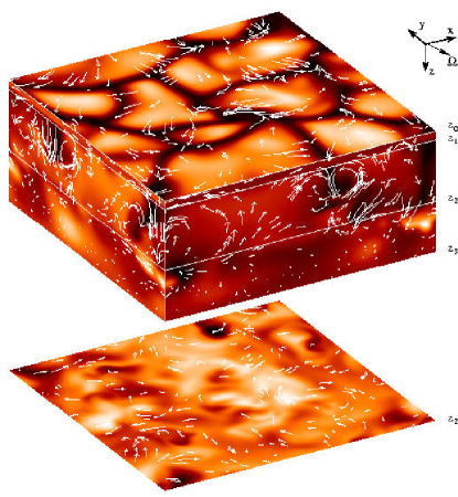
Figure 3: Snapshot of temperature fluctuations and velocity vectors from the run HICo1-30. At the top surface of the box we show horizontal contours at the $z=z_{1}$ plane and at the lower surface at the $z=z_{2}$ plane. The coordinate system and the direction of the rotation vector are shown in the upper right corner.

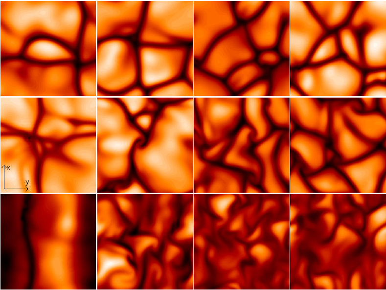
Figure 4: Horizontal cross-sections of temperature from fully developed convection at the top of the convectively unstable layer, $z=z_{1}$. From left to right, the individual frames are from latitudes $0$, $-30$, $-60$, and $-82.5$ degrees. The rotation rate increases from top to bottom, corresponding to sets Co01, Co1, and Co10. Here, the $x$-axis points to the east and the $y$-axis to the north.

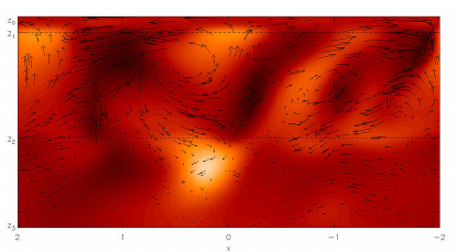
Figure 5: Vertical cross-section of temperature fluctuations and meridional velocity vectors in the $xz$-plane at $y=-1$ in the run Co7-60. The arrow at the upper right corner indicates the direction of the rotation vector.

5.1 Convective structures

To illustrate the general appearance of the structures arising in the present calculations we show a typical snapshot of temperature fluctuations overplotted with the velocity vectors from fully developed convection in a moderate rotation case HICo1-30 in Fig. 3. As in many previous studies we find a convection pattern dominated by broad warm upflows and narrow cool downflow plumes. Near the top the upflows form cells, separated from each other by a network of downflow structures at the cell boundaries. The downflow structures remain coherent over large depths, sometimes even extending over the whole convectively unstable layer. Generally, the horizontal scale of the convective pattern is observed to decrease as a function of depth. Note that the downflow lanes seen near the top tend to form a few well-defined plumes at larger depths and the regions of upward flow connect and become broader. However, the upflows also tend to become less well-defined, so that much more small-scale structure is seen as opposed to the large and well-defined ’granules’ near the top. Although this apparently contradicts the prediction of the mixing length theory, on average the upflows occupy a larger area in the deeper layers in accordance with the basic mixing length concept.

The effects of rotation can be studied from Fig. 4 where we show horizontal contours of temperature from three different calculation sets at four latitudes. In the weak rotation case (set Co01), shown in the uppermost row, the convective cells have more or less angular shapes, which pattern changes only slightly as function of latitude. There is a weak tendency of the sizes of the structures to get smaller towards the pole, which effect becomes more pronounced as the rotation is increased (the middle row, set Co1); the size of the structures clearly decreases as function of increasing latitude. The angular appearance of the cells also changes due to the strong vortical downflows which are generated by the interaction of the converging flow with the Coriolis force at the cell edges. In the rapid rotation case (the bottom row, set Co10) the convective pattern is dominated by rather irregular small-scale structures, except for the equatorial case, where the pattern is totally aligned with the rotation axis, reminiscent of the banana cells seen in some global convection models (e.g. Brun & Toomre BruTo02 (2002)). Such an alignment is a generic feature of the convective motions in the rapid rotation regime, as can be seen from Fig. 5, where $xz$-slices of temperature fluctuations overplotted with velocity field vectors are shown from the run Co7-60.

5.2 Velocity field characteristics

In Tables 1 and 2 we have calculated some diagnostics of the velocity field. Comparing the total and fluctuating rms-velocities (columns 6 and 7, respectively), one can note that both tend to decrease towards the poles and increase steeply near the equator for rapid rotation. A similar trend can be seen in the azimuthal and vertical velocity field components (columns 9 and 10). This is partly due to the fact that the convection is more efficient in the equatorial regions compared to the polar ones (see Sect. 5.4), partly because the increasing rotational influence generates azimuthal mean flows, seen as a deviation between the total and the fluctuation, which are strongest near the equator.

The degree of horizontal anisotropy, measured by the quantity

$$A_{H}=\frac{\langle u_{y}^{\prime 2}\rangle-\langle u_{x}^{\prime 2}\rangle}{u_{t}^{2}}\;.$$ (50)

is very small at all latitudes for the slow rotation cases (sets Co01 to Co1). As rotation is increased, $A_{H}$ obtains positive values near the equator due to the strong azimuthal mean flows generated there. However, the isotropy is more or less re-established at southern latitudes $\Theta>30\degr$, also for the rapid rotation cases.

The vertical component of the velocity is dominating over the horizontal ones for the slow rotation cases, which means that the preferred direction of the convective motions is the radial one, in which stratification and energy transport also occur. This anisotropy, measured by the quantity

$$A_{V}=\frac{\langle u_{y}^{\prime 2}\rangle-\langle u_{z}^{\prime 2}\rangle}{u_{t}^{2}}\;,$$ (51)

is observed to decrease as the rotational influence increases, because the convective structures become more and more aligned with the rotation vector. The sign of this quantity is also useful since it should coincide with the sign of the radial gradient of the angular velocity, $\frac{d\Omega}{dr}$ (Rüdiger Rudiger80 (1980)). In the present calculations, $A_{V}$ is almost always negative, except for the rapid rotation cases near the equator. Thus, the velocity anisotropy generated in our calculations reproduces the helioseismic result of positive $\frac{d\Omega}{dr}$ at the equator and at low latitudes and a negative one at higher latitudes only for the sets Co4 to Co10. However, we expect that this result is slightly affected by the fact that the averages were taken only over the convectively unstable region. In this case the flow regions where the vertical flows turn into horizontally diverging flows, mostly occurring in the upper boundary and overshoot layers, were excluded from the calculation, resulting in the overestimation of $u_{z}$ over $u_{y}$.

Figure 6: Volume-averaged kinetic helicity, $\mathcal{H}$, normalised by the maximum value, for the sets Co1 (dashed line) and Co10 (solid line). For comparison, the dotted line shows a $-\cos\theta$ profile and the dash-dotted line a $-\sin\theta$ profile multiplied by 0.65 in order to fit to the data.

Figure 7: Mean energy fluxes as functions of depth from the run Co1-30, normalised by the input flux, see Sect. 5.4 for definitions.

Figure 8: The Nusselt number as a function of Taylor (lower x-axis) and Coriolis (upper x-axis) numbers at different latitudes for the $\rm Ra=2.5\cdot 10^{5}$ (left) and $\rm Ra=10^{6}$ (right) calculations. Different linestyles are used for each latitude investigated, as indicated in the left panel.

5.3 Kinetic helicity

Column 11 in Tables 1 and 2 shows the volume averaged kinetic helicity, $\mathcal{H}$, defined by

$$\mathcal{H}=\langle(\nabla\times\@vec{u}^{\prime})\cdot\@vec{u}^{\prime}\rangle\;.$$ (52)

This quantity is interesting in that it is believed to play a major role in the dynamo theory, providing the so-called $\alpha$-effect, which describes the generation of large-scale poloidal magnetic fields due to the inductive action of helical turbulence. In the simplest approximation, making use of the first order smoothing and assumption of isotropy, $\alpha\approx-\frac{1}{3}\tau^{\prime}\mathcal{H}$, where $\tau^{\prime}$ is the correlation time associated with the turbulence. It has been noted that the $\alpha$ computed from magnetoconvection calculations qualitatively agrees with the above approximation (Ossendrijver et al. Osse01 (2001), Osse02 (2002)). Furthermore, it is possible to determine the sign and latitudinal distribution of the magnitude of $\mathcal{H}$ in the surface layers of the Sun from helioseismology (Duvall & Gizon DuGi00 (2000); see also Rüdiger et al. Rudetal99 (1999) who studied numerically the determination of $\mathcal{H}$ from surface flows). The aforementioned studies indicate that $\mathcal{H}$ is maximal at the poles with a nearly $\cos\theta$-latitude dependence. The sign of $\mathcal{H}$ is noted to be positive in the bulk of the convection zone in the southern hemisphere and negative in the northern hemisphere.

We find that on the low rotation calculations $\mathcal{H}$ shows several sign changes as function of depth so that the volume average is small and does not show a clear latitudinal trend. When rotation is moderate (sets Co1 to Co4) there is a clear tendency for the helicity to be positive in the convectively unstable region and to increase towards the pole (bar the Co4 set with Ra $2.5\cdot 10^{5}$), in accordance with the aforementioned studies. As function of depth, the positive values peak near the top of the convection zone while a region of smaller negative helicity resides in the overshoot layer. This region of negative $\mathcal{H}$ grows as rotation is increased so that for the strong rotation cases, only a narrow region of positive helicity remains in the surface layers. Near the equator, this positive peak dominates in the volume average of $\mathcal{H}$, but for latitudes $\Theta<-15\degr$ the sign is negative which behaviour carriers all the way to the pole, however, with monotonically decreasing absolute values (see Figure 6). Taken that the close relation between the helicity and the $\alpha$-effect persists in the rapid rotation regime, this would indicate that for strong enough rotation, the sign of the $\alpha$-effect changes from negative to positive and simultaneously decreases in magnitude at higher latitudes, whilst larger negative values occur in the equatorial regime. Interpreted in terms of the classical dynamo theory, in the regime of slow and moderate rotation, the poloidal field generation would be more efficient near the poles with equatorward migration of activity phenomena, when combined with the observed internal rotation law. In the rapid rotation regime, in contrast, the $\alpha$-effect would be more efficient in the equatorial regions, and the migration would be equatorward at low latitude regions and poleward at higher latitudes. However, the proportionality between $\mathcal{H}$ and the $\alpha$-effect is only approximate, and can yield incorrect results for realistic circumstances. Thus, calculations with magnetic fields are needed in order to determine whether the behaviour suggested by the helicity really occurs in the rapid rotation regime.

5.4 Convection efficiency

To show the energy transport in a typical calculation, we plot the depth dependence of the horizontally averaged energy fluxes in Fig. 7 for the run Co1-30. We define

$$F_{\rm rad} = \kappa\frac{\partial\langle e\rangle}{\partial z}\;,$$ (53)

$$F_{\rm conv} = -\gamma\langle\rho e^{\prime}u_{z}^{\prime}\rangle\;,$$ (54)

$$F_{\rm kin} = -\frac{1}{2}\langle\rho\@vec{u}^{2}u_{z}\rangle\;,$$ (55)

$$F_{\rm visc} = -2\nu\langle\rho S_{zi}u_{i}\rangle\;,$$ (56)

as the radiative, convective, kinetic, and viscous fluxes. The minus signs arise because we define positive flux to be directed outwards. Most of the energy is transported by radiative diffusion, whilst the convection transports roughly one fifth of the total energy flux through the convection zone. The flux of kinetic energy is directed downwards, and amounts to a few per cent of the total flux. The viscous flux is in all cases negligible. The change of sign of $F_{\rm conv}$ in the overshoot layer is due to the fact the negative temperature fluctuations entering the stable layer find themselves as positive fluctuations in the new background stratification. We find that the convective flux decreases as rotation is increased so that $F_{\rm conv}$ in the Co10 set is roughly half of that in the Co01 set.

The rotational influence on the convection efficiency can be estimated quantitatively by the Nusselt number, (see e.g. Brandenburg et al. Brand90 (1990))

$${\rm Nu}=\frac{F_{\rm tot}-F_{\rm ad}}{F_{\rm rad}^{(0)}-F_{\rm ad}}\;,$$ (57)

where $F_{\rm tot}=F_{\rm rad}+F_{\rm conv}+F_{\rm kin}+F_{\rm visc}$ is the total flux through the convectively unstable layer, $F_{\rm ad}=\kappa\big{(}\frac{\partial e}{\partial z}\big{)}_{\rm ad}$ the radiative flux if the layer is adiabatic, and $F_{\rm rad}^{(0)}=\kappa\frac{\Delta e}{\Delta z}$ the radiative flux if the temperature stratification in the unstable layer is linear. The Nusselt number gives the ratio of the total heat flux and the heat flux which would be transported by conduction alone. Thus Nu must exceed unity for convection to be present.

The resulting Nusselt numbers as functions of rotation, measured by Ta and Co, at the latitudes investigated are shown in Fig. 8. The slow rotation case Co01 does not show any definite latitudinal variation, which is indeed the expected behaviour. The variation seen within the set Co01 can then be used as an error estimate for the other sets. When the rotation is stronger, the efficiency of convection decreases as a function of latitude in a more or less monotonic fashion. Convection at equatorial regions seems to be most vigorous and for $\Theta\leq-45\degr$ the efficiency does not change appreciably as the latitude increases. The trend that convection at polar regions would be more vigorous than at some intermediate latitudes noted by Gilman (Gilman77 (1977)) and Pulkkinen et al. (Pulkki93 (1993)) is not observed here. Furthermore, we do not find a regime where Nu increases with increasing Ta (Hathaway & Somerville Hatha83 (1983)). For the $\rm Ra=10^{6}$ calculations the qualitative results are very similar, the distinction being the roughly 50% larger values of Nu.

5.5 Overshooting depth

Convective overshooting is thought to be important for example in the context of stellar magnetism providing means to store magnetic flux below the convection zone by resisting the buoyancy effect. In our calculations, indeed, the downflows very often overshoot into the stable layer below, where they decelerate due to the buoyancy force. We define the depth of overshooting as

$$d_{\rm os}=z_{2}-z_{\rm os},$$ (58)

where $z_{\rm os}$ is the depth where the horizontally averaged kinetic energy flux falls below a threshold value of $e^{-1}$ of its value at the bottom of the convectively unstable layer. In order to facilitate a comparison to a real star we normalise the overshooting depth by the pressure scale height, $H_{\rm p2}=e_{2}(\gamma-1)/g$, at the bottom of the convectively unstable layer.

The calculated depths for the Ra $=2.5\cdot 10^{5}$ runs are shown in the upper panel of Fig. 9 as functions of latitude and Coriolis number. As a general feature we find that the overshooting decreases as a function of increasing rotation at a given latitude. Such behaviour has earlier been reported by Brummell et al. (Brumm02 (2002)) and Ziegler & Rüdiger (ZieRu03 (2003)). For the slowest rotation investigated (set Co01) the overshooting extends rather deep, down to $0.4H_{\rm p2}$, and the latitude dependence is very weak as expected. For moderate rotation (sets Co05 to Co2) there is a clear trend of decreasing overshoot depth with latitude. However, as rotation is increased further, there is an opposite trend. At the poles, $d_{\rm os}$ seems to stay more or less constant, whilst it continues to decrease at the equator. This may be interpreted to be due to the stronger influence of the Coriolis force on the vertical downflows at the equatorial regions, where they tend to align with the rotation vector. The lower panel of Fig. 9 shows $d_{\rm os}$ as function of the Chandrasekhar number for the magnetic runs (see Sect. 5.7.4 for a detailed description of the runs). We find that the overshooting depth is reduced monotonically with increasing imposed field strength for the present range of parameters where the ratio of the gas to magnetic pressure in the bottom of the convection zone spans from $\approx 2.6\cdot 10^{5}$ to 260. Increase of $d_{\rm os}$ for small magnetic field strengths, noted by Ziegler & Rüdiger (ZieRu03 (2003)), is not observed.

For the most rapid rotation, $d_{\rm os}$ varies between about $0.1H_{\rm p2}$ at the equator to about $0.2H_{\rm p2}$ at high latitudes. This value is still larger than the estimates from helioseismology (e.g. Monteiro et al. Monte94 (1994)), but the rotational influence in our study is most probably still weaker than in the deeper layers of the solar convection zone. One must, however, bear in mind that the normalised energy flux, $F_{\rm tot}/\rho c_{\rm s}^{3}$, where $c_{\rm s}$ is the sound speed, at the bottom of the convectively unstable layer is roughly eight orders of magnitude larger than in the case of the sun. Furthermore, for non-rotating convection, the penetration depth scales with $u_{z}^{3/2}$ and the overshooting depth with the square root of the input flux (e.g. Zahn Zahn91 (1991); Hurlburt et al. Hurlburt94 (1994); Singh et al. Singh98 (1998)). The difference between penetration and overshooting is that the former extends the superadiabatic region and the latter does not. In the present calculations the thermal stratification does not appreciably change due to the overshooting and thus the latter scaling relation should be applicable. However, in our results no such scaling exists, since the input flux in the Ra=$10^{6}$ calculations is half the one used in the Ra=$2.5\cdot 10^{5}$ case but the overshooting depth decreases only by a factor of ten to fifteen per cent for the Co1 and Co4 sets and actually increases for the Co10 set (not shown). A possible explanation of this behaviour is that the mixing length theory, assumptions of which were used in the derivation of the scaling relation, breaks down when rotation is present. On the other hand, it has to be noted that our description of the overshoot region is not very realistic, the thermal diffusivity profile being essentially a smoothed step function, which quite probably acts to hinder the efficiency of overshooting in comparison to a smoothly varying profile.

5.6 Mean flows

Figure 9: Upper panel: overshooting depth, $d_{\rm os}$, as function of latitude for the calculations with Ra = $2.5\cdot 10^{5}$. Different linestyles are used for each set of calculations, differing by Coriolis number, as indicated in the figure. Lower panel: $d_{\rm os}$, as function of the Chandrasekhar number. The upper $x$-axis denotes the corresponding runs presented in Table 4.

Figure 10: Latitudinal (left) and azimuthal (right) mean flows, $\langle u_{x}\rangle$ and $\langle u_{y}\rangle$, respectively, plotted against depth from sets Co01 (top, slow rotation), Co1 (middle, moderate rotation), and Co10 (bottom, rapid rotation). The different linestyles correspond to different latitudes, which are denoted in the middle figure. On the lowest graph on the right, only a part of the equatorial azimuthal velocity is shown due to its large magnitude.

Figure 11: Reynolds stress components $\langle Q_{xy}\rangle/\nu_{t}$, $\langle Q_{yz}\rangle/\nu_{t}$, and $\langle Q_{xz}\rangle/\nu_{t}$ as functions of depth for the sets Co01 (top), Co1 (middle), and Co10 (bottom), respectively. Different latitudes are represented by the linestyles denoted in the middle figure.

The generation of differential rotation by the presence of anisotropic turbulence and uniform rotation is accounted for in the theory of the $\Lambda$-effect (e.g. R89) by the interaction of the anisotropic eddies with the Coriolis force. In the rectangular domain used in this study, this effect works to generate mean flows, of which of particular interest are the latitudinal and azimuthal ones which are indicative of the differential rotation in a full spherical domain. However, one must bear in mind that the boundary conditions in a spherical domain would permit a variety of other effects which affect the mean flows, such as horizontal temperature gradients, which in the present geometry could only be imposed and cannot arise naturally.

To investigate the depth dependence of the mean flows we average the horizontal velocities over a time period designated in Table 1 and over the horizontal directions. This procedure yields $\langle u_{x}\rangle(z)$ and $\langle u_{y}\rangle(z)$ for the latitudinal and azimuthal mean velocites, respectively, which are functions of $z$ alone. The vertical mean velocity $\langle u_{z}\rangle(z)$, calculated in this way, is very small in comparison to the horizontal ones due to the boundary conditions which do not permit a net vertical momentum flux. The fact that $\langle u_{z}\rangle$ still has a small finite value is due to the different filling factors of up- and downflows. Fig. 10 shows typical examples of these flows plotted at different latitudes for slow (Co01), moderate (Co1), and rapid rotation (Co10).

The predominant feature of the latitudinal flow for slow and intermediate rotation is the mostly negative (poleward) flow in the bulk of the convection zone and the positive (equatorward) flow in the overshoot layer. This trend is strongest for the set Co2, and when rotation increases, the latitudinal flow starts to diminish and the direction reverses for the most rapid rotation. For the rapid rotation cases (Co7 and Co10) there is a strong equatorward flow confined to a narrow layer near the surface and a much weaker poleward flow in the bulk of the convection zone. In the overshoot layer only a very weak equatorward flow is present.

The mean latitudinal flows in the slow rotation regime agree with the results of Chan (Chan01 (2001)) and Brummell et al. (Brumm98 (1998)). When rotation is stronger, the qualitative character of Chan’s results stays the same, in disagreement with ours, whereas in the study of Brummell et al. (Brumm98 (1998)) a sign change near the top of the domain is reported (their Fig. 6). The increasing magnitude of the latitudinal flow towards the equator noted by Brummell et al. (Brumm98 (1998)) is also present in our results for moderate rotation. However, the magnitude of the latitudinal flow in our study seems to grow for increasing rotation, a feature not present in the two aforementioned studies.

The azimuthal mean flow shows generally very similar behaviour, with increasingly negative values (westward motion) near the surface and smaller positive values (eastward) in the overshoot layer for slow and moderate rotation (up to the set Co2). The magnitude of the azimuthal flow decreases more or less linearly as function of depth, and also as function of increasing latitude. The latter effect is reminiscent of the Taylor-Proudman theorem (e.g. Chandrasekhar Chandra61 (1961)) which states that motions cannot vary in the direction of the rotation axis leading to cylinder shaped contours of the angular velocity. The former effect was discussed by Chan (Chan01 (2001)), who showed that the dominant term in the equation for the mean azimuthal flow at the equator is the horizontal component of the Coriolis force, $f_{\rm C}=2\,\Omega\cos\Theta u_{z}$, which produces a shear of approximate magnitude of

$$\frac{\Delta\langle u_{y}\rangle}{\Delta z}\approx 2\,\Omega\;,$$ (59)

where the difference $\Delta$ is taken over the unstable layer. Our results follow this relation for the slow and moderate rotation cases (sets Co01 to Co2), but this relation fails for the rapid rotation regime. However, a more general way of explaining the mean flows in the present calculations can be easily obtained by considering the Reynolds stresses, see Sect. 5.6.1 below.

Just as the latitudinal flow, also the azimuthal mean flow reverses direction in the bulk of the convection zone for the most rapid rotation (Co7 and Co10). There is also a moderate westward flow in the bulk of the convection zone and a layer of negative shear near the surface. A narrow layer of retrograde motion exists in the overshoot region. This behaviour is very similar to the investigations by Brummell et al. (Brumm98 (1998)) and Chan (Chan01 (2001)).

5.6.1 Generation of the mean flows by the Reynolds stresses

Next we study the horizontal momentum balance in the model by deriving the equations for the latitudinal, azimuthal, and vertical momentum balance, which are obtained by taking a horizontal average of the momentum equation, Eq. (3)

$$-\frac{\partial}{\partial z}(\langle\rho u_{x}u_{z}\rangle)-2\,\Omega\langle\rho u_{y}\rangle\sin\Theta = 0\;,$$ (60)

$$-\frac{\partial}{\partial z}(\langle\rho u_{y}u_{z}\rangle)+2\,\Omega\langle\rho u_{x}\rangle\sin\Theta = 0\;,$$ (61)

$$-\frac{\partial}{\partial z}(\langle\rho u^{2}_{z}\rangle)-2\,\Omega\langle\rho u_{y}\rangle\cos\Theta-\frac{\partial\langle p\rangle}{\partial z}+\langle\rho\rangle g = 0\;.$$ (62)

In the azimuthal equation we have dropped the Coriolis term involving the mean vertical momentum $\langle\rho u_{z}\rangle$, which vanishes due to the boundary conditions. Furthermore, applying the Reynolds rules, the remaining terms of the form $\langle u_{i}u_{j}\rangle$ can be expanded using Eq. (26). In this expansion terms with $\langle u_{z}\rangle$ appear, but these are very small in comparison to the other mean velocities and can be neglected. The remaining terms of Eqs. (60) to (62) can then be used to solve for the mean horizontal velocities

$$\langle u_{y}\rangle = -\frac{1}{2\,\Omega\langle\rho\rangle\sin\Theta}\frac{\partial}{\partial z}(\langle\rho\rangle\langle u^{\prime}_{x}u^{\prime}_{z}\rangle)\;,$$ (63)

$$\langle u_{x}\rangle = \frac{1}{2\,\Omega\langle\rho\rangle\sin\Theta}\frac{\partial}{\partial z}(\langle\rho\rangle\langle u^{\prime}_{y}u^{\prime}_{z}\rangle)\;,$$ (64)

$$\langle u_{y}\rangle = -\frac{1}{2\,\Omega\langle\rho\rangle\cos\Theta}\Big{[}\frac{\partial}{\partial z}(\langle\rho\rangle\langle u_{z}^{\prime 2}\rangle)+\frac{\partial\langle p\rangle}{\partial z}-\langle\rho\rangle g\Big{]}\;.$$ (65)

At the equator, the latitudinal mean flow vanishes due to symmetry, and Eq. (63) has a singularity. However, Eq. (65), which includes contribution of the diagonal Reynolds stress component $\langle u_{z}^{\prime 2}\rangle$ in the pressure field, can be used instead. We find that the vertical derivatives of the Reynolds stress components $\langle u^{\prime}_{y}u^{\prime}_{z}\rangle$ and $\langle u^{\prime}_{x}u^{\prime}_{z}\rangle$ explain the generated horizontal mean flows in all non-equatorial models. At the equator, Eq. (65) reproduces the observed zonal mean flow, and is applicable at all latitudes investigated. Thus, the observed mean flows in the models arise due to the non-vanishing transport of momentum driven by the Reynolds stresses as expected.

5.7 Reynolds stresses and the $\Lambda$-effect

In this section we discuss the spatial distribution of the Reynolds stress components generated in the calculations, and their dependence on rotation and large-scale magnetic fields. To draw conclusions of the effects of the generated stresses on the angular momentum transport and generation of differential rotation in a global spherical geometry, we parametrise the stresses in terms of the $\Lambda$-effect coefficients. This is also interesting because the calculations presented here are not restricted by the assumptions of FOSA, due to which the results may be used to test the validity of this approximation. It has to be born in mind, however, that our local calculations also have restrictions, including the effects of periodic horizontal boundaries, limited number of pressure and density scale heights included, and the small Reynolds and Rayleigh numbers, due to which the turbulence modelled is relatively weak and the convection rather inefficient.

5.7.1 The stresses due to the generated mean flows

As discussed in the previous section, mean flows exhibiting radial gradients naturally arise in the calculations due to the non-zero Reynolds stresses (they also vary as a function of latitude measured from different calculation sets, but due to the periodic horizontal boundaries the latitudinal gradients vanish in the calculations). In this case, in the series expansion of the Reynolds stresses, Eq. (33), the diffusive contribution will become non-zero as well, due to which it should be separated before calculating the $\Lambda$-coefficients, for which we have adopted the following procedure. Using the radial profiles of the latitudinal and azimuthal mean flows generated in the calculation of interest as an additional imposed velocity field component stationary in time (i.e. writing the velocity field as ($u_{x}+u_{x}^{\rm shear}(z)$,$u_{y}+u_{y}^{\rm shear}(z)$,$u_{z}$) and adding advection terms of types $u_{i}^{\rm shear}\partial u_{j}/\partial{x_{i}}$ and $u_{z}\partial u_{i}^{\rm shear}/\partial{z}$ to the equations), we repeat a few calculations switching off rotation, and calculate the generated Reynolds stresses. These stresses now correspond to the diffusive part in the series expansion, denoted here by $Q_{ij}^{(\rm shear)}$. Subtracting these stresses from the ones generated in the full calculations, we obtain the non-diffusive contribution

$$Q_{ij}^{(\Lambda)}=Q_{ij}^{(\rm tot)}-Q_{ij}^{(\rm shear)}\;.$$ (66)

We chose to apply this procedure only to a subset of the full calculations, namely for the sets Co1 and Co10, corresponding to moderate and rapid rotation, respectively, and at the latitudes of $0\degr$, $-7.5\degr$, $-30\degr$, and $-60\degr$; the results are summarised in Table 3.

We note that the stresses generated by the shear flows are largest in the cases where the imposed flows were taken from the equatorial or near-equatorial cases. The stress component $Q_{xy}^{(\rm shear)}$ is small in comparison to $Q_{xy}^{(\rm tot)}$ for all latitudes in the Co1 set (note that the stress components $Q_{xy}$ and $Q_{xz}$ should vanish at the equator due to symmetry). In the rapid rotation case $Q_{xy}^{(\rm shear)}$ is approximately one fifth of the total stress near the equator and about one eight for latitude $-30\degr$. For the other two latitudes the stresses are statistically consistent with zero. Since the contribution of the shear is of the same sign as the total, we note that it acts as to diminish the contribution of the $\Lambda$-effect. We thus conclude that the horizontal $\Lambda$-effect derived from the total stress is overestimated by maximally 20 per cent near the equator for the most rapid rotation cases.

The stress component $Q_{yz}$ shows an opposite trend: $Q_{yz}^{(\rm shear)}$ is in general of opposite sign to $Q_{yz}^{(\rm tot)}$ which indicates an underestimation of the vertical $\Lambda$-effect. This underestimation is largest near the equator due to the large azimuthal mean flows there (see Figure 10). Noteworthy is that the shear contribution is almost equal to the $\Lambda$ part at the equator for the Co10 case but for the latitude $-7.5\degr$ the shear contribution is already insignificant. In conclusion, the vertical $\Lambda$-effect estimated from $Q_{yz}^{(\rm tot)}$ is in general underestimated near the equator possibly by a factor of two to three but that this effect is significantly weaker for all higher latitudes, being maximally a few tens of per cents in the moderate rotation cases. The stress component $Q_{xz}^{(\rm shear)}$ is insignificantly small in comparison to $Q_{yz}^{(\rm tot)}$ for all non-equatorial cases studied.

Table 3: Comparison of the volume averaged Reynolds stresses generated by rotation and dynamically generated mean flows versus stresses generated by mean flows alone (in units of [$10^{-3}]$).

$$\begin{array}[]{p{0.24\linewidth}cccc}\hline\cr\vskip 3.0pt plus 1.0pt minus 1.0pt\cr Run&\langle Q_{xy}\rangle_{V}/\nu_{t}&\langle Q_{yz}\rangle_{V}/\nu_{t}&\langle Q_{xz}\rangle_{V}/\nu_{t}\\ \vskip 3.0pt plus 1.0pt minus 1.0pt\cr\hline\cr Co1-00&-0.09&\ \ 1.60&-0.03\\ Co1-00-shear&\ \ 0.06&-1.37&-0.06\\ Co1-7.5&-4.83&\ \ 3.10&-4.59\\ Co1-7.5-shear&-0.12&-1.17&-0.37\\ Co1-30&-0.86&\ \ 7.28&-6.64\\ Co1-30-shear&\ \ 0.07&-0.44&-0.20\\ Co1-60&-0.56&\ \ 7.15&-4.87\\ Co1-60-shear&\ \ 0.04&\ \ 0.01&-0.13\\ \hline\cr Co10-00&\ \ 0.72&-2.53&\ \ 0.19\\ Co10-00-shear&-1.39&\ \ 7.03&-0.09\\ Co10-7.5&\ \ 27.4&-9.39&-1.53\\ Co10-7.5-shear&\ \ 5.70&\ \ 0.07&\ \ 0.04\\ Co10-30&\ \ 8.68&-3.19&-8.76\\ Co10-30-shear&\ \ 1.00&\ \ 0.05&-0.58\\ Co10-60&\ \ 2.62&-0.28&\ \ 4.02\\ Co10-60-shear&\ \ 1.74&\ \ 0.30&-0.15\\ \vskip 3.0pt plus 1.0pt minus 1.0pt\cr\hline\cr\end{array}$$

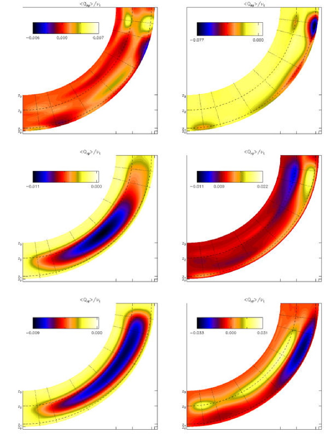
Figure 12: A polar representation of the horizontally averaged Reynolds stress components $\langle Q_{\theta\phi}\rangle$ (top), $\langle Q_{r\phi}\rangle$ (middle), and $\langle Q_{r\theta}\rangle$ (bottom), normalised by the turbulent viscosity. Data from the sets Co1 (left) and Co10 (right) is shown. The dashed lines denote the top and bottom of the convectively unstable layer, and the dotted lines indicate the latitudes for which data exists; to represent the latitudinal dependence of the stresses smoothly, a cubic spline interpolation between the datasets has been made. Note that the stresses are presented as they would appear in spherical coordinates on the southern hemisphere.

Figure 13: The volume averaged Reynolds stress components $\langle Q_{\theta\phi}\rangle$ (left), $\langle Q_{r\phi}\rangle$ (middle), and $\langle Q_{r\theta}\rangle$ (right) in units of $[10^{-2}]$, from the Ra = $2.5\cdot 10^{5}$ calculations, normalised by $\nu_{\rm t}\Omega$. The errorbars are calculated from Eq. (30). For comparison, the dashed lines show the results of KR93 for the corresponding Coriolis number.

Figure 14: Same as Fig. 13, but for the Ra $=10^{6}$ calculations.

5.7.2 Radial distribution

We continue by discussing the vertical (radial) profiles of the Reynolds stresses as the Taylor number is varied. These are shown for the horizontally averaged off-diagonal Reynolds stress components, normalised by an estimate of the turbulent viscosity $\nu_{t}=\frac{1}{3}u_{t}d$, in Fig. 11 for slow (set Co01), moderate (Co1), and rapid rotation (Co10). In order to visualise the latitudinal variation of the stresses, the data from the two latter sets are shown in a polar plot in Fig. 12.

The horizontal component, $\langle Q_{xy}\rangle$, shows several sign changes as function of depth and no clear trends are apparent for slow rotation (sets Co01 to Co05). For moderate rotation (Co1 and Co2) larger negative values tend to occur in the convection zone near the equator. For more rapid rotation, this latitudinal trend is more pronounced, and as a function of depth, a positive peak near the upper boundary develops. The magnitude of this feature increases with increasing rotation. A smaller positive peak develops in the overshoot region for the rapid rotation cases. The uppermost panels of Fig. 12 show more clearly the tendency of $\langle Q_{xy}\rangle$ to obtain its largest value near the equator. The maxima of $\langle Q_{xy}\rangle$ also tends to occur in the regions where the vertical flow is deflected to the horizontal directions, namely in the overshoot layer immediately below the convection zone and near the upper boundary.

The vertical Reynolds stress component, $\langle Q_{yz}\rangle$, shows a distinct trend of being mostly positive in the bulk of the convection zone for the slow and moderate rotation. Considerably weaker positive values of the stress occur in the overshoot region for these cases. The magnitude of this component increases up to the set Co2, after which the trend begins to change and for the set Co4 this quantity is more or less zero in the bulk of the convection zone near the equator (the positive peak in the overshoot layer remains) and the overall magnitude at other latitudes decreases. Similar trend continues in the set Co7. There is a sign change in the bulk (but not in the stable region) for the most rapid rotation (set Co10). As the latitude increases, the negative dip near the top of the domain becomes narrower.

The meridional component of the stress, $\langle Q_{xz}\rangle$, is negative throughout the domain for the slow rotation cases Co01 to Co1. The magnitude of this quantity is less in the overshoot region than in the bulk of the convection zone. For the set Co2 the same trend continues on the lower latitudes but there is a sign change at higher latitudes. With even more rapid rotation, $\langle Q_{xz}\rangle$ still exhibits a negative dip in the unstable region, but in addition a comparable positive peak appears in the overshoot region.

In comparison, the depth dependencies of the Reynolds stresses are in many cases at variance with those obtained by Chan (Chan01 (2001)). The accordance seems to be the best for the slow rotation cases ($\rm Co\leq 1$) and for the components $\langle Q_{yz}\rangle$ and $\langle Q_{xz}\rangle$. The sign changes observed when the rotation becomes large enough are seen to occur in the results of Chan (Chan01 (2001)) only for $\langle Q_{xy}\rangle$, whereas in our case all components exhibit this behaviour. The differences here also reflect the variance seen in the mean velocities.

Figure 15: Coefficients $H$ (left) and $V$ (right) from different latitudes as function of the Taylor number.

5.7.3 Latitudinal distribution

Figs. 13 and 14 depict the volume averages of the Reynolds stresses normalised by $\nu_{\rm t}\Omega$ as functions of latitude for all sets of calculations. We have adopted spherical coordinates in order to facilitate comparisons with other studies. Here we give an error estimate using a modified mean error of the mean, Eq. (30). For comparison, we show the results of KR93 for the corresponding Coriolis number for each set.

We begin our analysis from the horizontal component $\langle Q_{\theta\phi}\rangle_{V}$ (shown in the left columns of Figs. 13 and 14), which shows a lot of scatter and the errorbars are large for the slow rotation cases $\rm Co<1$; it seems that no real effect is present for these cases. As the rotation is increased, a trend starts to appear: the sign of the stress is negative at all latitudes, and the maximal magnitude is obtained at the latitude of $\Theta=-7.5^{\degr}$ accompanied by a rapid increase near the equator and a slower decrease when moving towards the poles; a series expansion in increasing powers of $\sin^{2}\theta$ traditionally used in describing the latitudinal distribution (e.g. R89) fits poorly to these profiles (not shown). This behaviour is very similar to the one reported by Pulkkinen et al. (Pulkki93 (1993)) for $\rm Co\approx 5$ in our notation, and visible also in the results of Chan (Chan01 (2001)).

For this stress component observations from the Sun exist (e.g. Ward Ward65 (1965); Virtanen Virtanen89 (1989)). On the sun $\langle Q_{\theta\phi}\rangle_{V}$ is negative on the southern hemisphere with a more or less a linear variation as a function of latitude (Pulkkinen & Tuominen Pulkki98 (1998)). The negative sign indicates that there is an angular momentum flux towards the equator. Qualitative correspondence with the observations is fairly good when $\rm Co\geq 2$.

A comparison with KR93 shows that, for the moderate rotation cases, the sign of $\langle Q_{\theta\phi}\rangle_{V}$ is the same in both studies, but that the latitudinal distribution is much more concentrated towards the equator in the present results. Also the magnitude of the horizontal $\Lambda$-effect, $H\equiv\frac{\langle Q_{\theta\phi}\rangle_{V}}{\nu_{t}\cos\theta\Omega}$, seems to be larger in our case. We find that the absolute value of $\langle Q_{\theta\phi}\rangle_{V}$ increases up to the set Co7, but the growth seems to have saturated for the set Co10, where the magnitude is comparable to the Co7 set. What this implies is that $H$ itself is decreasing as function of $\Omega$ for the most rapid rotation cases. This is an indication of rotational quenching of the horizontal $\Lambda$-effect, see the left panel of Fig. 15, which is noticiable when $\rm Co\geq 4$. Recent observational studies of rapidly rotating stars seem to support the view that generation of horizontal differential rotation is strongly suppressed when rotation is large enough (e.g. Reiners & Schmitt 2003b ).

The stress component $\langle Q_{r\phi}\rangle_{V}$ (the middle columns of Figs. 13 and 14) describes the radial flux of angular momentum, and is thus vital in generating radial differential rotation. We find that $\langle Q_{r\phi}\rangle_{V}$ is mostly negative, corresponding to inward transport of angular momentum, for all sets except the case Co01, where no clear trend is seen and the two most rapid rotation cases where a change of sign occurs. The magnitudes at the midlatitudes tend to be the largest for all the sets up to Co4. As the rotation is increased further, the sign changes, starting from the equatorial regions so that for the set Co10, $\langle Q_{r\phi}\rangle_{V}$ is positive at all latitudes, and obtains the maximum near the equator. The qualitative picture of $\langle Q_{r\phi}\rangle_{V}$ for the sets Co1 to Co4 is in accord with Pulkkinen et al. (Pulkki93 (1993)) and Chan (Chan01 (2001)), whereas on the rapid rotation end we seem to have come to a regime not yet encountered in the other studies. A comparison to the results of KR93 seems to support this view as well. The relatively strong and positive vertical $\Lambda$-effect of KR93 for slow rotation is not present in our results. When rotation is intermediate (sets Co2 and Co4), the correspondence is rather good, but the sign change at high rotation is not seen in the study of KR93. We note here that absolute value of $\langle Q_{r\phi}\rangle_{V}$ does not change appreciably from the set Co2 to Co10, which means that the vertical $\Lambda$-effect $V=\frac{\langle Q_{r\phi}\rangle_{V}}{\nu_{t}\sin\theta\Omega}$ is also subject to strong rotational quenching, and that this effect is much more clear for $V$ than for $H$ (see the right panel of Fig. 15).

Finally, the Reynolds stress capable of driving meridional flow, $\langle Q_{r\theta}\rangle_{V}$, does not show as clear trends as the two other components. For slow rotation (sets Co01 to Co1) this component is negative at all latitudes. For moderate rotation (set Co2), the values near the pole start to get positive. Towards the rapid rotation end, there seems to be a negative dip at low latitudes ($\Theta\approx-15\degr\ldots-30\degr$) and a positive one at high latitudes ($\Theta\approx-60\degr$). This qualitative trend is again similar to what Pulkkinen et al. (Pulkki93 (1993)) find in their study.

Our main conclusions for the Reynolds stress components relevant for the generation of differential rotation indicate that the angular momentum is transported towards the equator when rotation is significant (cases Co1 and up) and radially inwards for slow and moderate rotation (sets Co05 to Co4), and outwards for rapid rotation (sets Co7 and Co10). The efficiency of the angular momentum transport is largest at mid-latitudes for slow and moderate rotation and near the equator for the rapid rotation cases.

The observed rotational quenching of the $\Lambda$-coefficients is of great interest in the context of the dynamo theory, where the generation of the toroidal magnetic field occurs via the $\Omega$-effect, dependent on the absolute differential rotation $\Delta\Omega$. According to our results the generators of the $\Omega$-effect may be significantly reduced, the quenching of the $V$ coefficients being stronger and taking place with lower rotation rates than for the $H$ coefficients. This implies that the horizontal differential rotation would dominate over the radial one in stars with moderate rotation rates, but that even the horizontal differential rotation would diminish significantly in the rapid rotation regime. Therefore, the dynamos operating in rapidly rotating stars can be expected to be of $\alpha^{2}$-type. One must, however, note that the $\alpha$-effect is probably, at least at the poles, subject to rotational quenching as well (Ossendrijver et al. Osse01 (2001)). It remains to be seen how the reverse of the sign and latitude distribution of the helicity noted in Sect. 5.3 in the rapid rotation regime changes this picture.

Table 4: Summary of the calculations with an imposed azimuthal magnetic field.

$$\begin{array}[]{p{0.04\linewidth}cccccccccccc}\hline\cr\vskip 3.0pt plus 1.0pt minus 1.0pt\cr Run&{\rm Ch}&{\rm Rm}&H_{\rm tot}[10^{-2}]&V_{\rm tot}[10^{-1}]&M_{\rm tot}[10^{-2}]&{\rm E_{kin}}\;[10^{-3}]&{\rm E_{mag}/E_{kin}}&{u_{t}}&{b_{t}}&A_{H}\;[10^{-3}]&A_{V}\;[10^{-3}]&\Delta T/\tau\\ \vskip 3.0pt plus 1.0pt minus 1.0pt\cr\hline\cr M0&0&-&\;\;\;4.38&-3.67&-5.80&2.03&-&0.085&-&1.6&-12.1&108\\ M1&1&141&-0.01&-3.57&-2.41&1.98&0.22&0.084&0.009&1.5&-12.1&57.8\\ M2&10&133&\;\;\;2.26&-3.90&-6.77&1.74&0.50&0.079&0.021&2.8&-13.0&54.4\\ M3&10^{2}&129&-2.94&-5.41&\;\;\;8.27&1.51&1.04&0.073&0.035&3.5&-10.8&50.5\\ M4&10^{3}&119&-9.38&-5.90&-8.86&1.43&4.15&0.071&0.042&16.0&\;\;\;7.9&47.7\\ \vskip 3.0pt plus 1.0pt minus 1.0pt\cr\hline\cr\end{array}$$

Figure 16: The volume averages of the rms-velocities (left) and rms-magnetic fields (right) in different directions.

Figure 17: Vertical profiles of the horizontally averaged total turbulent stresses $\langle T_{ij}\rangle$ normalised by the turbulent viscosity from the magnetic runs M0 to M4 transformed into spherical coordinates.

Figure 18: $\Lambda$-coefficients $H_{\rm tot}$, $V_{\rm tot}$, and $M_{\rm tot}$ as functions of the normalised field strength, $\beta_{m}=|\@vec{B}|/\sqrt{\mu_{0}\rho u_{t}^{2}}$. The quenching functions derived by Kitchatinov et al. (1994b ) are overplotted with the dotted linesymbols (see Sect. 5.7.4 for explanations).

5.7.4 The effect of an imposed azimuthal magnetic field

We investigated the behaviour of the total turbulent stresses, defined as

$$T_{ij}=Q_{ij}-(\mu_{0}\rho)^{-1}M_{ij},$$ (67)

where $Q_{ij}$ and $M_{ij}$ are the corresponding Reynolds and Maxwell stress tensor components, in the magnetic regime by a set of calculations (listed in Table 4) in which we impose a large-scale azimuthal magnetic field ${\@vec{B}}=(0,B_{0}=\rm const,0)$ of varying strength on top of a convection pattern at a saturated state. This choice seems plausible since the dominating component of the solar mean magnetic field is the toroidal one. Since the imposed field has no gradients, the large-scale Lorentz-force vanishes in the calculations, whilst the Maxwell stresses are non-zero due to the turbulent magnetic field component generated when the convective turbulence is acting on the mean field. We define the modified $\Lambda$-coefficients including the effect of the Maxwell stresses as

$$H_{\rm tot} = -\frac{\langle T_{xy}\rangle_{V}}{\nu_{t}\cos{\theta}\Omega}\>,$$ (68)

$$V_{\rm tot} = -\frac{\langle T_{yz}\rangle_{V}}{\nu_{t}\sin{\theta}\Omega}\>,$$ (69)

$$M_{\rm tot} = \frac{\langle T_{xz}\rangle_{V}}{\nu_{t}\sin{\theta}\cos{\theta}\Omega}\;,$$ (70)

and list the values obtained from the calculations in the columns 4, 5, and 6 of Table 4.

As a base calculation for this study we took the run Co2-60, where all the Reynolds stress components were appreciably large. The maximum Chandrasekhar number was chosen to be $10^{3}$ (run M4) which corresponds to a situation where the magnetic energy is roughly four times the kinetic energy of turbulence (Table 4, column 8) in the saturated state. This calculation can be thought to represent the superequipartition case, whereas M3 corresponds to equipartition.

When a magnetic field is imposed on top of the convection pattern, the flow undergoes a transition stage of a few tens of time units, after which it relaxes to another stable state; in measuring the quantities listed in Table 4 we have neglected this transition phase. Due to the convective motions acting on the magnetic field, a fluctuating magnetic field is generated. The strength of the fluctuating field (measured by the rms-alue listed in column 10) grows roughly exponentially up to M3, after which the growth seems to become quenched. For the runs M1 to M3 the fluctuating field is dominating over the large-scale field, although the fraction of small-scale energy over the large-scale one is decreasing nearly exponentially when the strength of the imposed field is increased. For the run M4 the large-scale field is dominating over the fluctuating one and also tends to elongate convective structures along its direction. The total and fluctuating velocity fields, measured by the total kinetic energy and the rms-value listed in columns 7 and 9, respectively, become suppressed by the magnetic field, as expected; from M1 to M3 the suppression is, again nearly exponential, but seems to cut off for M4.

Due to the presence of the imposed azimuthal field, an additional anisotropy is induced to the system. The azimuthal magnetic field is excerting a force opposing the movements in the directions perpendicular to it, which is seen as the suppression of the latitudinal and vertical velocity components, whilst the azimuthal velocity component is less affected (see Fig. 16 panel on the left). For the largest field strength (run M4) the azimuthal velocity exceeds the other components, indicating that motions occur mostly along the field lines in contrast to the non-magnetic case (M0) in which the vertical (radial) direction was preferred. This anisotropy is also seen in the quantities $A_{H}$ and $A_{V}$ listed in columns 11 and 12, defined by Eqs. (50) and (51); the former is obtaining larger positive values as the magnetic field strength grows, the latter smaller negative values and finally changing sign when the azimuthal motions grow larger than the radial ones. The fluctuating magnetic field components (see Fig. 16 panel on the right) generated by the convective motions rather closely reflect this anisotropy bar the run M4, so that, e.g., the velocity component containing the most of energy generates the strongest fluctuating magnetic field in its direction.

The generated total turbulent stresses $T_{ij}$, plotted in Fig. 17, show rather an unexpected behaviour. Although, in general, the fluctuating velocity field becomes suppressed, the turbulent correlations are rather enhanced in magnitude when the strength of the imposed field is increased. In the hydrodynamic case M0, the stress components responsible for the generation of differential rotation, $\langle T_{r\phi}\rangle$ and $\langle T_{\theta\phi}\rangle$, are negative throughout the domain, the former being the strongest in magnitude. For this component the profile retains its shape in the magnetic regime, only the magnitude increasing as magnetic field grows. The growth is accompanied by the increase of the mean latitudinal flow $\langle u_{x}\rangle$, so that it is roughly twice as strong in the case M4 than in M0. The two weak negative peaks seen in $T_{\theta\phi}$ develop in a less systematic manner, the one at the interface of the convective and overshoot layers remains more or less unaffected by the growing magnetic field, but the one near the surface changes its sign and gains in magnitude. The behaviour of $T_{r\theta}$ does not show any clear trend, but changes its magnitude, profile and sign rather irregularly. The mean azimuthal flow, generated by the $r\theta$ component, also lacks a systematic behaviour, although it tends to change its sign averaged over depth, being preferably positive in the regime of strong magnetic field.

The coefficients $H_{\rm tot}$, $V_{\rm tot}$, and $M_{\rm tot}$, calculated from the horizontal averages of the total stresses, are plotted in Fig. 18 as functions of the normalised field strength $\beta_{m}=|\@vec{B}|/\sqrt{\mu_{0}\rho u_{t}^{2}}$, where $|\@vec{B}|=B_{0}+b_{t}$. In the hydrodynamic case M0 (see Fig.13 fourth row) the horizontal $\Lambda$-coefficient is positive, whilst the vertical coefficient and the quantity $M$ are negative. As the magnetic field is applied to the system, the horizontal coefficient changes its sign and increases monotonically in magnitude (the dashed line in Fig. 18), the growth being somewhat reduced in the run M4. The vertical coefficient (the solid line) retains its negative sign, and also shows a monotonic increase in magnitude, with less evident signs of a suppression of the growth in the strong field limit. No obvious trend is visible for the quantity $M$ (dashed-dotted line), as already implied by the irregular behaviour of the stress $\langle T_{r\theta}\rangle$.

Figure 19: Volume averaged eddy heat flux tensor components $\chi_{rr}/\chi_{t}$ (left), and $\chi_{\theta r}/\chi_{t}$ (right) as functions of latitude for the Ra $=2.5\cdot 10^{5}$ runs. The errorbars denote the modified mean error of the mean as calculated from Eq. (30).

Figure 20: Same as Fig. 19 but for the Ra $=10^{6}$ sets.

As a comparison, we have overplotted the quenching functions for the weak field limit $\beta_{m}\ll 1$ derived by Kitchatinov et al. (1994b ) in Fig. 18 (dotted lines). Their derivation is made in the limit of slow rotation for arbitrary field strength, due to which the results are not very well compatible with our moderate rotation case with $\rm Co=2$, but nevertheless provide useful comparison with the analytical turbulence models. In the hydrodynamical slow rotation limit, the vertical coefficient is predicted to be positive (see the dashed lines plotted in the first row of Fig. 13 or Fig. 2 of KR93), whilst the horizontal coefficient vanishes. The inclusion of a weak magnetic field causes the appearance of an additional horizontal component negative in sign, which is enhanced as the magnetic field grows $(\propto\beta_{m}^{2})$, except for the strong field regime, where the coefficient becomes quenched $(\propto\beta_{m}^{-3})$. In our case, the horizontal component is clearly enhanced, even so that the growth exceeds the prediction of the analytical model (plotted on top with the dotted line, scaled to match the sign and hydrodynamical value of the calculated $H$-profile) and also shows a sign change compared to the hydrodynamic case, but the signs are reversed in comparison to the analytical results. Although the growth becomes somewhat suppressed in the strong field limit, it is significantly milder than predicted by the analytical investigation. A quenching function of a similar form (plotted on top of the calculated $V$-profile with a dotted line, scaled to match the hydrodynamical value) was derived for the vertical component, accompanied by a sign change from positive to negative with increasing magnetic field. In our calculations the vertical component remains negative and increases in magnitude as function of $\beta_{m}$. The growth is also much stronger than the one predicted by the analytical expression and no significant quenching, as expected from the analytical theory ($\propto\beta_{m}^{-3}$), however, is found in the strong field regime.

In summary, the produced set of magnetic runs with an imposed azimuthal field indicate that the $\theta\phi$ and $r\phi$ components of the turbulent stresses, capable of generating horizontal and vertical differential rotation, respectively, increase in magnitude with increasing imposed field strength whilst the $r\theta$ component, capable of affecting the meridional circulation pattern, shows no clear trends although also gains its maximum value for the case of the strongest magnetic field. The model setup, however, hardly represents the situation in a real stellar convection zone, where magnetic fields arise due to the turbulent convective and large-scale shearing motions, exhibiting gradients and thereby mean electric currents leading to the Malkus-Proctor effect, which has been excluded from this investigation.

5.8 Turbulent heat transport

In Figs. 19 and  20 we show the latitudinal variation of the volume averaged eddy heat flux tensor components $\chi_{rr}$ and $\chi_{\theta r}$, defined via Eq. (45). We use an estimate of the turbulent conductivity $\chi_{t}=\nu_{t}$ as normalisation. The error is estimated as in Figs. 13 and 14.

The radial component $\chi_{rr}$ is always positive, indicating that the heat flux is directed radially outwards, except at the equator for the case of highest rotation (Co10-00). In this calculation the temperature stratification becomes distorted by the strong rotational influence so that $\delta_{r}$ becomes negative. The latitudinal trends for $\chi_{rr}$ are clear: maximum occurs at the equator with diminishing magnitude towards the pole and with increasing rotation rate. There seems to be, in general, a tendency for the minimum to occur at a latitude $\Theta\approx-45\degr\ldots-60\degr$, indicating a minimum in the efficiency of convection. These trends concur with the ’deeper layer’ results of Pulkkinen et al. (Pulkki93 (1993)). However, the occurence of the minimum in the turbulent heat flux at mid-latitudes seems to contradict the one obtained from the Nusselt numbers (see Fig. 8), which indicates that the efficiency of convection decreases monotonically from the equator towards the pole. This discrepancy can be explained as follows: the value of the Nusselt number, Eq. (57), depends on only $F_{\rm rad}^{(0)}=\kappa\frac{\Delta\langle e\rangle}{\Delta z}$, where the difference $\Delta$ is taken using the values at the layers $z_{1}$ and $z_{2}$. In other words, the temperature stratification is assumed to be linear. If this was true, the radial superadiabacity, $\delta_{r}$, would be proportional to $F_{\rm rad}^{(0)}$, and the latitudinal profiles of $\chi_{rr}$ would show the same qualitative trend as the Nusselt number since $\langle u_{z}^{\prime}T^{\prime}\rangle$ itself and Nu show similar tendencies as function of latitude. The superadiabatic layer, however, gets shallower from the equator to the pole, which affects $F_{\rm rad}^{(0)}$ immediately because it depends only on the values of $e$ at depths $z_{1}$ and $z_{2}$. On the other hand, the convection zone is more superadiabatic (i.e $\delta_{r}$ is larger) at mid-latitudes than near the poles. Since $\chi_{rr}$ takes into account the whole stratification rather than just the endpoints, it probably gives a more reliable estimate of the convection efficiency than the Nusselt number does.

The $\chi_{\theta r}$ component shows a less coherent picture. For slow and moderate rotation $\chi_{\theta r}$ is negative throughout the latitude range, the maximum being at low latitudes ($\Theta\approx-10\ldots-30\degr$). For the case Co4 $\chi_{\theta r}$ obtains positive values near the pole and for the higher rotation cases there is a definite positive peak at high latitudes, and another near the equator.

Due to the boundary conditions we cannot actually have a temperature difference between the top layers of the boxes situated at different latitudes, but the radial gradient and the value at the bottom of the box are not constrained. In accordance with the latitudinal distribution of $\chi_{rr}$, we find that the temperature gradient in the equatorial cases is always shallower than at higher latitudes, and that the mid-latitudes do seem to be the least favoured in the sense that there the gradient is the steepest. If this situation was naively moved onto a spherical star where we assume the core to have a constant surface temperature below the convection zone, this would result in a warm equator and pole, and a cooler region at mid-latitudes. However, this approach is probably too simple since it does not take into account the latitudinal transport which shows a more complex pattern. For slow rotation (Co01 to Co1), the negative values of $\chi_{r\theta}$ indicate an equatorward heat flux at all latitudes. In the intermediate regime (Co2 and Co4) there is a poleward flux at the polar regions and a less pronounced equatorward one near the equator, supporting the view of the cooler mid-latitudes discussed above. This tendency, however, is reversed in the rapid rotation regime, so that a poleward flux appears at the equatorial regions, and an equatorial one at high latitudes, which kind of a flux would act as smoothing out the latitudinal temperature difference generated by the radial heat flux.

6 Conclusions

We have performed local three-dimensional hydrodynamical calculations of compressible convection with the inclusion of an overshoot layer in Cartesian volumes placed at various latitudes and with largely varying rotation. We find that the convective structure changes from an ordered cellular pattern of slow and moderate rotation (Co $\leq 2$) to a highly irregular small-scale pattern for rapid rotation (Co $\geq 4$). The efficiency of convection is noted to, in general, decrease as function of increasing rotation, while the latitudinal dependence indicates a minimum at mid-latitudes and more efficent convection at the equator and near the poles.

The kinetic helicity, $\mathcal{H}$, shows a similar trend as previous numerical studies of magnetoconvection (e.g. Ossendrijver et al. Osse02 (2002)) and helioseismic inversions (Duvall & Gizon DuGi00 (2000)) or large positive values at the south pole and an approximately $\cos\theta$-latitude dependence for slow and moderate rotation. We, however, find that for rapid enough (Co $\geq 4$) rotation the sign of the helicity changes and the latitudinal distribution follows more a $\sin\theta$-dependence at latitudes $\Theta\leq-15\degr$ than the $\cos\theta$-profile typical for the two aforementioned studies. It has been concluded that the $\alpha$ computed from magnetoconvection calculations qualitatively agrees with the first order smoothing result $\alpha\approx-\frac{1}{3}\tau^{\prime}\mathcal{H}$ (e.g. Ossendrijver et al. Osse01 (2001)). If this behaviour carries over to the rapid rotation regime, the $\alpha$-effect would also be subject to a sign change and simultaneous decrease of magnitude at higher latitudes.

The convective overshooting is reduced monotonically as a function of rotation. The latitudinal dependence shows two regimes; (i) for slow and intermediate rotation the overshooting depth decreases as latitude increases, and that (ii) for rapid rotation the trend is the opposite. Imposing an azimuthal magnetic field causes the overshooting depth to decrease monotonically as a function of increasing field strength.

The mean flows, generated by the Reynolds stresses, also show two distinct regimes; in cases of slow and intermediate rotation the latitudinal flow is poleward and the azimuthal one retrograde. Both components exhibit a more or less linear shear profile in the convectively unstable region. For rapid rotation, the signs of the mean flows change so that there is a strong equatorward flow in a narrow region near the surface and a weak poleward flow in the bulk of the convection zone. The azimuthal flow is prograde in the bulk and with a retrograde dip near the upper boundary.

The volume-averaged Reynolds stress components, $\langle Q_{\theta\phi}\rangle_{V}$ and $\langle Q_{r\phi}\rangle_{V}$, responsible for the generation of horizontal and vertical differential rotation, respectively, indicate that the angular momentum is transported equatorwards in all cases where rotation is significant (a positive horizontal $\Lambda$-effect). The radial transport occurs inwards (negative vertical $\Lambda$-effect) for slow and moderate rotation and towards the surface for rapid rotation (positive vertical $\Lambda$-effect). The latitudinal distribution shows that the inward transport in situated mostly at high latitudes and the outward transport near the equator. The meridional Reynolds stress component, $\langle Q_{r\theta}\rangle_{V}$ is negative for slow rotation and reaches positive values at high latitudes near the pole. We find that both $\Lambda$-effects are subject to rotational quenching, indicating the suppression of differential rotation in rapidly rotating stars. Comparison to the analytical turbulence model of KR93, based on the quasi-linear approach, shows a rather close agreement for the horizontal $\Lambda$-effect near the polar regions, whilst the values obtained from our calculations are systematically larger near the equator and less suppressed as the rotation is increased. The regime of positive vertical $\Lambda$-effect for slow rotation is not found from our calculations, but for intermediate rotation the agreement with KR93 is fairly good. For the rapid rotation regime, however, the positive vertical $\Lambda$-effect obtained in this study is in disagreement with the analytical theory.

We have also produced a set of magnetohydrodynamical calculations by imposing a mean azimuthal magnetic field on a saturated convection pattern with $\rm Co=2$. As the imposed field does not have any gradients, no mean currents are present in the system, due to which the large-scale Lorentz force vanishes. The action of the convective motions on the mean azimuthal field, however, leads to the generation of a fluctuating component of the magnetic field and non-zero Maxwell stresses. In the magnetohydrodynamical regime both the Reynolds and Maxwell stresses contribute to the angular momentum transport; the magnitude of the total turbulent stresses is observed to increase monotonically, although the turbulent velocity field, in general, becomes suppressed. The horizontal $\Lambda$-effect is observed to change sign from positive to negative as the field strength increases, indicating a new regime of poleward transport due to the presence of the magnetic field.

The turbulent heat transport indicates a rather strong latitudinal dependence of the radial heat flux, whereas the latitudinal flux shows no distinct tendencies. A simple analysis of the radial heat flux indicates that the equatorial regions should be the warmest, followed by the polar regions, and a cool belt at mid-latitudes would appear. However, this interpretation is most probably based on too simple assumptions since the thermal structure is also affected by the latitudinal heat flux and the meridional circulation. On the other hand, the latter depends on the thermal structure so a straightforward analysis as above is inadequate.

Having the knowledge of the Reynolds stresses and turbulent heat transport as functions of rotation and latitude it is, in principle, possible to investigate the implications of these local results on the global dynamics (rotation law, thermal structure) by utilizing a mean-field model in a spherical geometry. However, this analysis is not within the scope of this paper.

- (1) Bonanno, A., Elstner, D., Rüdiger, G. and Belvedere, G. 2002, A&A, 390, 673
- (2) Brandenburg, A., Nordlund, Å., Pulkkinen, P., Stein, R. F. & Tuominen, I. 1990, A&A, 233, 277
- (3) Brandenburg, A., Moss, D., Tuominen, I. 1992 A&A, 265, 328
- (4) Brandenburg, A., Jennings, R. L., Nordlund, Å., et al. 1996, JFM, 306, 325
- (5) Brandenburg, A., Käpylä, P. J. & Mohammed A. 2004, Physics of Fluids, 16, 1020
- (6) Brummell, N. H., Hurlburt, N. E. & Toomre, J. 1998, ApJ, 493, 955
- (7) Brummell, N. H., Clune, T. L. & Toomre, J. 2002, ApJ, 570, 825
- (8) Brun, A. S. & Toomre, J. 2002, ApJ, 570, 865
- (9) Collier Cameron, A., 2002, AN, 323, 336
- (10) Caunt, S. E. & Korpi, M. J. 2001, A&A, 369, 706
- (11) Chan, K. L. & Sofia, S. 1986, ApJ, 307, 222
- (12) Chan, K. L. 2001, ApJ, 548, 1102
- (13) Chandrasekhar, S. 1961, Hydrodynamic and Hydromagnetic Stability (Oxford: Clarendon)
- (14) Donahue, R. A., Saar, S. H. & Baliunas, S. L. 1996, ApJ, 466, 384
- (15) Duvall, T. L. Jr. & Gizon, L. 2000, Solar Phys., 192, 177
- (16) Gilman, P. A. 1977, Geophys Astrophys Fluid Dyn., 8, 93
- (17) Hall, D. 1991, in: The Sun and Cool Stars: activity, magnetism, dynamos, IAU Coll. 130, eds. I. Tuominen, D. Moss & G. Rüdiger, Lecture Notes in Physics 380 (Springer)
- (18) Hathaway D. H. & Somerville R. C. J., 1983, JFM, 126, 75
- (19) Henry, G. W., Eaton, J. A., Hamer, J. & Hall, D. S. 1995, ApJS, 97, 513
- (20) Hurlburt, N. E., Toomre, J., Massaguer, J. M. & Zahn, J. P. 1994, ApJ, 421, 245
- (21) Jennings, R. L., Weiss, N. O. 1991, MNRAS 252, 249
- (22) Kichatinov, L. L. & Rüdiger, G. 1993, A&A, 276, 96 (KR93)
- (23) Kitchatinov, L. L., Pipin, V. V. & Rüdiger, G. 1994a, AN, 315, 157
- (24) Kitchatinov, L. L., Rüdiger, G. & Küker, M. 1994b, A&A, 292, 125
- (25) Kichatinov, L. L. & Rüdiger, G. 1995, A&A, 299, 446
- (26) Kichatinov, L. L. & Rüdiger, G. 1999, A&A, 344, 911
- (27) Küker, M., Rüdiger, G. & Kichatinov, L. L. 1993, A&A, 279, L1
- (28) Küker, M., Rüdiger, G. & Pipin, V. V. 1996, A&A, 312, 615
- (29) Küker, M., Arlt, R. & Rüdiger, G. 1999, A&A, 346, 922
- (30) Küker, M. & Stix, M. 2001, A&A, 366, 668
- (31) Monteiro, M. J. P. F. G., Christensen-Dalsgaard, J. & Thompson, M. J. 1994, A&A, 283, 247
- (32) Ossendrijver, M., Stix, M. & Brandenburg, A. 2001, A&A, 376, 726
- (33) Ossendrijver, M., Stix, M., Brandenburg, A. & Rüdiger, G., 2002, A&A, 394, 735
- (34) Pipin, V. V. 1999, A&A, 346, 295
- (35) Pulkkinen, P., Tuominen, I., Brandenburg, A., Nordlund, Å. & Stein, R. F. 1993, A&A, 267, 265
- (36) Pulkkinen, P. & Tuominen, I., 1998, A&A, 332, 755
- (37) Reiners, A. & Schmitt, J. H. M. M. 2003a, A&A, 398, 647
- (38) Reiners, A. & Schmitt, J. H. M. M. 2003b, A&A, 412, 813
- (39) Rieutord, M., Brandenburg, A., Mangeney, A. & Drossart, P. 1994, A&A, 286, 471
- (40) Robinson, F. J. & Chan K. L. 2001, MNRAS, 321, 732
- (41) Rüdiger, G. 1977, AN, 298, 245
- (42) Rüdiger, G. 1980, Geophys. Astrophys. Fluid Dyn. 16, 239
- (43) Rüdiger, G. 1989, Differential rotation and stellar convection: Sun and solar-type stars, Akademie-Verlag, Berlin (R89)
- (44) Rüdiger, G. & Kichatinov, L. L. 1992, A&A, 269, 581
- (45) Rüdiger, G., Brandenburg, A. & Pipin V. V. 1999, AN, 320, 135
- (46) Schou, J. S., Antia, H. M., Basu, S. et al. 1998, ApJ, 505, 390
- (47) Singh, H.P., Roxburgh, I. W. & Chan, K. L. 1998, A&A, 340, 178
- (48) Stix, M. 1972, A&A, 37, 121
- (49) Stix, M. 2002, The Sun: An introduction, Second Edition, Springer-Verlag, Berlin Heidelberg New York
- (50) Thompson, M. J., Christensen-Dalsgaard, J., Miesch, M. S. & Toomre, J. 2003, ARA&A, 41, 599
- (51) Tuominen, I. & Rüdiger, G. 1989, A&A, 217, 217
- (52) Virtanen, H., 1989, Licentiate thesis, University of Helsinki
- (53) Ward, F. 1965, ApJ, 141, 534
- (54) Zahn, J. P. 1991, ApJ, 252, 179
- (55) Ziegler, U. & Rüdiger, G. 2003, A&A, 401, 433