CMB Observations and the Production of
Chemical Elements at the End of the Dark Ages

The metallicity evolution and ionization history of the universe must leave its imprint on the Cosmic Microwave Background through resonant scattering of CMB photons by atoms, ions and molecules. These transitions partially erase original temperature anisotropies of the CMB, and also generate new fluctuations. In this paper we propose a method to determine the abundance of these heavy species in low density (over-densities less than $10^{4}-10^{5}$) optically thin regions of the universe by using the unprecedented sensitivity of current and future CMB experiments. In particular, we focus our analysis on the sensitivity of the PLANCK HFI detectors in four spectral bands. We also present results for l=220 and 810 which are of interest for balloon and ground-based instruments, like ACT, APEX and SPT. We use the fine-structure transitions of atoms and ions as a source of frequency dependent optical depth ($\tau_{\nu}$). These transitions give different contributions to the power spectrum of CMB in different observing channels. By comparing results from those channels, it is possible to avoid the limit imposed by the cosmic variance and to extract information about the abundance of corresponding species at the redshift of scattering. For PLANCK HFI we will be able to get strong constraints ($10^{-4}-10^{-2}$ solar fraction) on the abundances of neutral atoms like C, O, Si, S, and Fe in the redshift range 1-50. Fine-structure transitions of ions like CII, NII or OIII set similar limits in the very important redshift range 3-25 and can be used to probe the ionization history of the universe. Foregrounds and other frequency dependent contaminants may set a serious limitation for this method.

1 Introduction

High precision observations of CMB anisotropies are giving us unique information about the angular distribution of CMB fluctuations, as well as their spectral dependence in a very broad frequency range. HFI and LFI detectors of PLANCK spacecraft will provide unprecedented sensitivity in 9 broad band $(\Delta\nu/\nu\sim 20-30\%)$ channels, uniformly distributed in the spectral region of the CMB where contribution of different foregrounds are expected to be at a minimum. CMBpol and other proposed missions are expected to reach noise levels 20 - 100 times lower than that of PLANCK HFI with technology already available (Church 2002). The WMAP satellite was designed to provide measurements of the CMB temperature anisotropies in the whole sky with an average sensitivity of 35$\mu$K per $0.3^{\circ}\times 0.3^{\circ}$ pixel at the end of the mission (Bennett et al. 2002, Page et al. 2002). Once such sensitivity limit is reached, the WMAP data will be the first real-life test for all those attempts to estimate, with extremely high precision, the key parameters of our universe using this sensitivity (Bond, Efstathiou & Tegmark 1997, Einsestein, Hu & Tegmark 1999, Prunet, Sethi & Bouchet, 2000). Indeed, after the first 12 months of operation, the WMAP team is recovering the first multipoles of the CMB power spectrum with an accuracy of a few percent (Hinshaw et al. 2003).

In this paper we are presenting an additional use of the tremendous sensitivity of PLANCK and CMBpol, and ground-based experiments like ACT, APEX and SPT. We propose to look for or to place upper limits on the abundances of heavy elements present in the inter galactic medium and/or in optically thin clouds of gas everywhere in the redshift range $[1,500]$. We shall focus on the fine-structure lines of neutral (CI, OI, SiI, FeI, …) and ionized (CII, NII, OIII, …) atoms, which might provide information about the epoch of first star formation and ionization history of the universe. Limits on abundances of heavy atoms and ions can be obtained by utilizing the frequency dependent opacity that will be generated by scattering of background photons by these species; giving rise to different $\delta C_{l}$-s in in different observing bands of the experiments. Although Planck HFI is expected to detect the combined signal from the strongest lines, like OI $63.2\mu$, CII $157.7\mu$ and OIII $88.4\mu$, future multichannel broadband CMB anisotropy experiments like CMBpol might permit to detect contributions from these lines separately from the epoch when dark ages were terminating, universe became partially ionized and heavy element production begun. It is important that the polarization signal arising due to resonance scattering depends strongly on the properties of the transition (Sazonov et al. 2002), and together with the temperature signal will permit us to separate contributions of different species.

The observed primordial acoustic peaks and angular fluctuations should not depend on the frequency at all. This is connected with the nature of Thomson scattering which produces these fluctuations both in the time of recombination of hydrogen in the universe (Peebles & Yu 1970, Sunyaev & Zel’dovich 1970) and during the secondary ionization of the universe (Sunyaev 1977, Ostriker & Vishniac 1986, Vishniac 1987, and more recently Gruzinov & Hu 1998, da Silva et al. 2000, Seljak, Burwell & Pen 2000, Springel, White & Hernquist 2001, and Gnedin & Jaffe 2001). In this context, WMAP polarization measurements have recently shown strong evidence favouring an early reionization scenario, with $z_{r}=20^{+10}_{-9}$ (Kogut et al. 2003, 95% confidence). But if any amount of chemical elements are present during the dark ages, then these species will be able to scatter the CMB in their fine-structure lines. This scattering would not only partially smooth out primordial CMB anisotropies, but in addition will generate new fluctuations through the Doppler shift of the line associated with the motion of matter connected with the growth of density perturbations. The main difference with Thompson scattering is that the latter is giving us equal contribution over the whole CMB spectrum, whereas the discussed line scattering would give different contribution to different observing channels placed at different parts of the spectrum. Likewise, the contribution in this case would be restricted to a very thin slice in the universe. Hence there is a possibility to detect contribution from the lines with high transition probabilities, even though the typical optical depth we would find is very small ($\tau_{\nu}<10^{-4}$). Since every line is able to work only in a given range of redshift, having observations on different wavelengths can give an upper limit to abundances of different species at different epochs. This method relies critically in the fact that intrinsic CMB temperature fluctuations are frequency independent. Therefore, in the absence of other frequency-dependent components, the difference of two CMB maps obtained at different frequencies must be sensitive to the difference in abundance of resonant species at those redshifts probed by the frequency channels. For this reason, this method is particularly sensitive to the possible presence of any frequency-dependent signal coming from foregrounds.

The idea to use the line transitions of atoms and molecules for modifying the CMB power spectrum is not new. Dubrovich (1977, 1993) proposed the use of rotational lines of primordial molecules (LiH, HD etc.) as a source of creating new angular fluctuations in the CMB, and there have been attempts to observe these molecules at high redshifts (de Bernardis et al. 1993). Varshalovich, Khersonskii and Sunyaev (1978) were trying to estimate the spectral distortions of CMB due to absorption in fine-structure lines of oxygen and carbon at redshifts around 150-300 where the temperature of electrons should be lower than the temperature of CMB due to different adiabatic indices of radiation and matter (see Zel’dovich, Kurt & Sunyaev 1968). Suginohara et al.(1999) probed the possibility of detecting excess flux due to emission in these lines coming from very over-dense regions in the universe. Recently Loeb (2001) and Zaldarriaga & Loeb (2002) (hereafter ZL02) computed the distortions connected with the recombination of primordial Lithium and scattering in the Lithium resonant doublet line. Unfortunately the wavelength of fine-structure 2P-2S transition of Lithium atoms is too short and will be unobservable by PLANCK and balloon instruments. On the very low frequency domain, future experiments like SKA and LOFAR might detect signal from neutral hydrogen 21 cm line, which also carry important ioformation from high redshifts (Sunyaev & Zel’dovich 1975, Madau, Meiksin & Rees 1997). We consider below the ground-state fine-structure lines of heavier elements, with wavelengths of the order of $50-200\mu$, which will in principle be observable with PLANCK and CMBpol if they are present in the redshift range $[1,500]$. The problem of overcoming their extremely small optical depth comprises the main idea of this paper.

We will not discuss in detail the origin and ways of enrichment of the inter-galactic gas by heavy elements. This certainly requires existence of massive stars, supernova explosions, stellar and galactic winds, and even jets from disks around young stars with cold molecular gas (Yu, Billawala & Bally 1999). The main goal of this paper is to show that the announced sensitivity of PLANCK detectors might permit us to set very strong upper limits to the time of enrichment of inter-galactic gas by heavy elements, the time of reionization, and maybe even to detect the heavy elements in the inter-cluster medium. The census of baryons in the local universe (Fukugita et al. 1998) shows that most of the baryon remains unobserved, and the proposed method might set way to detect its existence at high redshifts, when it had moderate or low temperature. These missing baryons are centainly out of stars, interstellar gas and intergalactic gas in clusters and groups of galaxies. However, we know that such baryons should exist because they have been detected by WMAP at the last scattering surface at $z\simeq 1100$, and are also necessary to justify the observed abundance of deuterium and ⁶Li in the early universe. Due to the wide range of redshifts under study, and the uncertain degree of mixture and clumpiness of our species in the interstellar and inter-galactic medium, we shall assume that all elements are smoothly distributed in the sky. In other words, in the present paper we shall address exclusively the homogeneous low density optically thin case, where effects related to strong over-density of gas and collisional excitation are excluded and left as subject of an upcoming work. Resonant scattering effects will produce the discussed signal even if all the gas in the enriched plasma has over-density up to $10^{3}$. Under this smooth approximation, we will find that the effect of resonant species on the CMB power spectrum will be particularly simple, especially in the high multipole range. Indeed, in the small angular scales, we shall show that the induced change in the $C_{l}$’s is given by $\delta C_{l}\simeq-2\;\tau_{X_{i}}C_{l}$, where $\tau_{X_{i}}$ is the optical depth induced by the resonant scattering of species $X$ and $C_{l}$ is the primordial CMB power spectrum, which is currently the main target of most CMB experiments.

In section 2 we describe the basic approach for computing optical depths and corresponding deviations in the CMB power spectra due to scattering, and then show how we can put constraints on abundances using the sensitivity of present and future CMB experiments. Section 3 presents our main results for atoms and ions, and in section 4 we discuss various possible ionization and enrichment scenarios of the universe and the nature of predicted signal for each case. We will demonstrate in the Appendix B that optically thin over-dense regions with $\langle n_{e}\rangle<10-200$ cm^-3 are contributing to the effect of resonant scattering. The effect of foreground emissions on our analysis is discussed in section 5, and we conclude in section 6. Throughout this paper we have used the parameters for standard $\Lambda\mbox{CDM}$ cosmology (Spergel et al. 2003), with $\mbox{H}_{0}=71\ km\ s^{-1}\ Mpc^{-1},\ \ \Omega_{b}=0.044,\ \ \Omega_{m}=0.27,\ \Omega_{\Lambda}=0.73,\ \mbox{and}\ \tau_{T}=0.17$ for secondary reionization. $\mbox{T}_{0}$ is the present-day value of mean CMB temperature, given by $\mbox{T}_{0}=2.726\mbox{K}$ (Mather et al. 1994).

2 Basic Approach

We now discuss the basic method of obtaining the deviations in the CMB power spectrum by resonance scattering of atoms and ions, and using this deviation to constrain their abundance during the dark ages. The interaction of CMB photons with atoms and ions will mostly consist of resonant scattering with either an atomic or a rotational/vibrational transition, depending on the species under study. In the Appendix A we detail how we introduce the optical depth due to the resonant transition ($\tau_{X_{i}}$) in the CMBFAST code (Seljak & Zaldarriaga, 1996). We consider a particular resonant transition $i$ for a given species $X$, with rest-frame resonant frequency $\nu_{i}$. The total optical depth encountered by CMB photons on their way from the last scattering surface to us is then obtained by adding the contributions from all lines to the standard Thomson opacity:

$$\tau=\tau_{T}+\sum_{i}\tau_{X_{i}}$$ (1)

In order to calculate $\tau_{X_{i}}$, we shall recur to the formula which gives the optical depth of a resonant transition in an expanding medium (Sobolev 1946),

$$\tau_{X_{i}}(z)=f_{i}\ {\frac{\pi e^{2}}{m_{e}c}}{\frac{\lambda_{i}n_{X_{i}}(z)}{H(z)}},$$ (2)

where $f_{i}$ is the absorption oscillator strength of the resonant transition, $\lambda_{i}$ is the corresponding wavelength (in rest frame), $n_{X_{i}}(z)$ is number density of $X$ species at redshift $z$, and $H(z)$ is the Hubble parameter at that epoch. The oscillator strength depends on $\lambda_{i}$, the Einstein coefficient of the transition $A_{ul}$, and the degeneracy of the levels involved in it:

$$f_{i}=\frac{m_{e}c}{8\pi^{2}e^{2}}\frac{g_{u}}{g_{l}}\ \lambda_{i}^{2}A_{ul}$$ (3)

A simple and elegant treatment following Gunn & Peterson (1965) using $\delta$-function line profile, instead of thermally broadened gaussian for the same line, gives same value of optical depth. Further modifications are made to this formula to take into account the finite populations in the upper transition levels, which is important for atomic fine-structure transitions, where excitation temperature for them is comparable to the radiation temperature at high redshifts. Also the effect of non-zero cosmological constant can not be neglected in the low redshift universe of interest. Considering these facts, we obtain the following formula for optical depths:

$$\tau_{X_{i}}(z)\ =\ 1.7\times 10^{-6}\ \left(\frac{{\cal X}_{X_{i}}(z)}{10^{-6}}\right)\ \ \times$$

$$\phantom{xxxxxxxxxxxx}\times\ \left({\frac{{\cal S}(z)}{{\cal S}(z=10)}}\right)\ \left(\frac{\lambda_{i}}{100\ \mu}\right)\ \left(\frac{f_{i}}{10^{-9}}\right)\ {\cal B}.$$ (4)

Here ${\cal X}_{X_{i}}(z)$ is the ratio between the number density $N_{X_{i}}(z)$ of the atomic or ionic species $X$ under consideration, with respect to the baryon number density at the same redshift: $N_{b}(z)=2\times 10^{-7}\;(1+z)^{3}$ cm^-3. i.e. ${\cal X}_{X_{i}}(z)=N_{X_{i}}/N_{b}$ presents the evolution of abundance of the given species due to element production, ionization and recombination processes. We propose to constrain the minimum abundance that can be detected at that redshift in solar units, or $[X]_{min}\equiv{\cal X}_{X_{i}}(z)\;/\;{\cal X}_{\odot}$, where, for example, ${\cal X}_{\odot}=3.7\times 10^{-4}$ for carbon. ${\cal S}(z)$ gives the redshift dependence of optical depth in a $\Lambda$CDM universe: ${\cal S}(z)=(1+z)^{3}\ [(1+z)^{2}(1+\Omega_{m}z)-z(2+z)\Omega_{\Lambda}]^{-\frac{1}{2}}$ (see, e.g., Bergstrom 1998) , and $\lambda_{i}$ is the wavelength in micron. The final term ${\cal B}$ accounts for the actual fraction of atom/ion present in their ground state, and is governed solely by the temperature of background radiation at the redshift of scattering. For a two-level system, this fraction is simply

$$n_{l}=[1+(g_{u}/g_{l})\ \exp(-h\nu_{i}/kT_{0}(1+z))]^{-1}.$$ (5)

We also include here the correcting term for the induced emission in the presence of the CMB and finite population of the upper level:

$${\cal B}=n_{l}\ \times\ \left[1-\exp{\left(-\frac{h\nu_{i}}{k_{B}T_{0}(1+z)}\right)}\right].$$ (6)

The resonance scattering on ions and atoms in thermal equilibrium with black body radiation does not change its intensity. However, the observed CMB also has finite primordial angular fluctuations. The effect of resonant scattering is to decrease these angular fluctuations, and to bring the system more close to thermodynamic equilibrium. Therefore resulting fluctuations observed on the frequency of the line should differ from the situation on other frequencies which are far from the resonance.

At low multipoles peculiar motions arising due to the growth of large scale density perturbations become important. All ions or atoms are moving in the same direction and change the frequency of CMB photons during resonant scattering. This leads to generation of new anisotropies of background.

We next give a simple description of the modification of the power spectrum of the CMB when it encounters a resonant species. As mentioned in the Introduction, our first hypothesis will be that the species responsible for the scattering are homogeneous, isotropic and smoothly (i.e., not clumped) distributed in the Universe, at least during the epoch of interaction with the CMB. One may argue that heavy species are located in halos where the first stars are produced and that their distribution in the sky can non be regarded as smooth. In this case, the final effect would depend on the typical angular size of the patches in which the species have been spread and on their total sky coverage. This paper will observe the case where those scattering patches percolate in the sky, giving rise to a smooth, homogeneous picture. The case of patchy distribution of emitting sources will be addressed in a forthcoming work, where collissional processes are studied in an extremely dense optically thick environment.

In the conformal Newtonian gauge, (also known as the longitudinal gauge), the k-mode of the photon temperature fluctuation at current epoch is given by (Hu & Sugiyama 1994)

$$\Delta_{T}(k,\eta_{0},\mu)\ =\ \int_{0}^{\eta_{0}}d\eta\;e^{ik\mu(\eta-\eta_{0})}\bigl{[}\Upsilon(\eta)\left(\Delta_{T0}-i\mu v_{b}\right)$$

$$\phantom{xxxxxxxxxxxxxxxxxxxxxxxxxxxxxxxx}+\ \dot{\phi}+\psi-ik\mu\psi\bigr{]}.$$ (7)

Here we have neglected the polarization term (which contributes at most with a few percent of the temperature amplitude). $\eta$ denotes the conformal time, $\Upsilon\equiv{\dot{\tau}}(\eta)\exp{-\tau(\eta)}$ is the visibility function and $\tau(\eta)=\int_{\eta}^{\eta_{0}}d\eta^{\prime}\dot{\tau}(\eta^{\prime})$ is the optical depth. $\Delta_{T0}$ accounts for the intrinsic temperature fluctuations, $v_{b}$ for the velocity of baryons and $\phi$ and $\psi$ are the scalar perturbations of the metric in this gauge. We have also neglected all tensor perturbations. If we now introduce the optical depth associated to a resonant transition as a Dirac delta of amplitude $\tau_{X_{i}}$ placed at $\eta=\eta_{X_{i}}$,

$$d\tau(\eta)=\sigma_{T}n_{e}(\eta)d\eta+\tau_{X_{i}}\delta(\eta-\eta_{X_{i}})d\eta,$$ (8)

we readily obtain that the original anisotropies have been erased by a factor $e^{-\tau_{X_{i}}}$, whereas new anisotropies have been generated at the same place:

$$\Delta_{T}(k,\eta_{0},\mu)\;=\;e^{-\tau_{X_{i}}}\Delta_{T_{orig}}(k,\eta_{X_{i}},\mu)\;+\;\Delta_{T_{new}}(k,\eta_{X_{i}},\mu)$$ (9)

In real space, if we assume that $\tau_{X_{i}}\ll 1$ , the Dirac delta approximation for the resonant transition (eq.(8)) translates into

$$\frac{\delta T}{T_{0}}({\bf n},z=0)=\left(1-\tau_{X_{i}}\right)\;\frac{\delta T}{T_{0}}({\bf n},z_{X_{i}})$$

$$\phantom{xxxxxxxxxxx}+\tau_{X_{i}}\;\frac{\delta T}{T_{0}}\biggr{|}_{new}^{lin}({\bf n},z_{X_{i}})\;+\;{\cal O}\left[\tau_{X_{i}}^{2}\right].$$ (10)

Here, ${\bf n}$ is the unitary vector denoting the observing direction, and $\delta T/T_{0}|_{new}^{lin}({\bf n},z_{X_{i}})$ is the linear in $\tau_{X_{i}}$ term of the newly generated anisotropies. We remark again that we are assuming that the species is homogeneously distributed, so that $\tau_{X_{i}}$ does not depend on position. Let us now consider two different observing frequencies: the first one corresponds to the scattering redshift $z_{X_{i}}$, and the another corresponds to a scattering redshift too high to expect any significant presence of the species $X$. If we compute the correlation function, $\bigl{<}\frac{\delta T}{T_{0}}({\bf n_{1}},z=0)\cdot\frac{\delta T}{T_{0}}({\bf n_{2}},z=0)\bigr{>}$, in both cases, we find that the difference of these quantities will be equal to:

$$\Delta\left(\bigl{<}\frac{\delta T}{T_{0}}({\bf n_{1}},z=0)\cdot\frac{\delta T}{T_{0}}({\bf n_{2}},z=0)\bigr{>}\right)=$$

$$\phantom{xxxxxxx}\tau_{X_{i}}\biggl{(}-\;2\;\bigl{<}\frac{\delta T}{T_{0}}({\bf n_{1}},z_{X_{i}})\cdot\frac{\delta T}{T_{0}}({\bf n_{2}},z_{X_{i}})\bigr{>}\;$$

$$\phantom{xxxxxxx}+\;2\;\bigl{<}\frac{\delta T}{T_{0}}({\bf n_{1}},z_{X_{i}})\cdot\frac{\delta T}{T_{0}}\biggr{|}_{new}^{lin}({\bf n_{2}},z_{X_{i}})\bigr{>}\biggr{)}+{\cal O}\left[\tau_{X_{i}}^{2}\right].$$ (11)

That is, the term linear in $\tau_{X_{i}}$ of $\Delta\left(\bigl{<}\frac{\delta T}{T_{0}}({\bf n_{1}},z=0)\cdot\frac{\delta T}{T_{0}}({\bf n_{2}},z=0)\bigr{>}\right)$ is the sum of two different contributions: the suppression of original fluctuations (which, as we shall see, dominates at small angular scales), and the cross-correlation of the newly generated anisotropies with the intrinsic CMB field. The first term (suppression) does not depend on the potential or velocity fields during scattering, but only on the intrinsic CMB anisotropy field. Moreover, we must remark that those contributions are evaluated at scattering epoch. Hence, if the resonant scattering takes place before reionization, the changes in the correlation function (or in the power spectrum, as we show below) will be sensitive to the CMB anisotropy field before being processed by the re-ionized medium. In the Appendix A we give a detailed computation of the change in the power spectrum due to a resonant line. As we concentrate in the optically thin limit, it is possible to make a power expansion on the optical depth $\tau_{X_{i}}$:

$$\delta C_{l}\equiv C_{l}^{X_{i}}-C_{l}=\tau_{X_{i}}\cdot{\cal C}_{1}+\tau_{X_{i}}^{2}\cdot{\cal C}_{2}+{\cal O}(\tau_{X_{i}}^{3}).$$ (12)

In this equation, $C_{l}^{X_{i}}$ and $C_{l}$ refer to the angular power spectrum multipoles in the presence and in the absence of the $X_{i}$ resonant transition, respectively. For the limit of very small $\tau_{X_{i}}$ one can retain only the linear order, and a direct identification of $\delta C_{l}$ with the abundance $[X](z)$ is possible by means of eq.(4): the change induced in the CMB power spectrum will be proportional to the abundance of the species responsible for the resonant scattering. In agreement with what has been established when studying $\Delta\left(\bigl{<}\frac{\delta T}{T_{0}}({\bf n_{1}},z=0)\cdot\frac{\delta T}{T_{0}}({\bf n_{2}},z=0)\bigr{>}\right)$, we find that ${\cal C}_{1}$ changes sign at some multipole $l_{cross}$: positive values of $\delta C_{l}$ imply generation of new anisotropies ($l<l_{cross}$), whereas anisotropies are suppressed for $l>l_{cross}$ (see figure 1 at very low $l$). In the Appendix A we note that positive values of $\delta C_{l}$ (generation) are due to the non-zero correlation existing between anisotropies generated during recombination and those generated during the resonant scattering. This correlation is due to the coupling of $k$ modes of the initial metric perturbation field in scales of the order or larger than the distance separating the two events (recombination at redshift $1100$ and resonant scattering at redshift $5$-$25$), (Hernández–Monteagudo & Sunyaev, in preparation).

\psfrag{123456789l}{Multipole, $l$}\psfrag{123456789123456789cl}{$l(l+1)/2\pi\ C_{l}\ \ (\mu K^{2})$}\psfrag{123456789log}{log($[\mbox{O}]_{min}/[\mbox{O}]_{\odot}$)}\includegraphics[width=298.75394pt,height=199.16928pt]{dev-hfi-O63.eps}

Figure 1: The nature of temperature anisotropy that will be marginally detectable with Planck HFI 143 GHz channel, using $63\mu$ OI line. Abundance is taken from the table(1), as $5.3\times 10^{-4}$ solar at redshift 32. Here Primary denotes the measured temperature anisotropy (upper line), $C_{l}^{pri}+\delta C_{l}\approx C_{l}^{pri}$, and Line denotes the the newly generated anistropy, $|\delta C_{l}|$, arising from line scattering (bottom, with filled squares). This $|\delta C_{l}|$ is obtained by taking the difference from the 100 GHz channel, and changes sign around $l=3$. The corresponding noise level is denoted by HFI noise. Also shown is the cosmic variance limit (short-dashed line) for comparison.

2.1 $\delta C_{l}$’s at small angular scales

With respect to the high-l range, we find that the change induced in the power spectrum takes a very simple form:

$$\delta C_{l}\simeq-2\;\tau_{X_{i}}\;C_{l}$$ (13)

where $C_{l}$ is the intrinsic power spectrum. This dependence is identical to the effect of reionization on the power spectrum at small angular scales. Indeed, in that scenario, if the optical depth due to electron scattering during this epoch is given by $\tau_{reio}$, then we have that for $l\gg 1$ the intrinsic CMB power spectrum generated at recombination is suppressed by a factor $1-\exp({-2\tau_{reio}})$, or $\approx-2\tau_{reio}$ if $\tau_{reio}<1$. So in both (resonant and Thompson) scatterings, the shape of the induced change in the power spectrum is particularly simple and equal to $\delta C_{l}\simeq-2\tau\;C_{l}$, for a given optical depth $\tau$ and intrinsic power spectrum $C_{l}$. This simplifies considerably the effect of reionization on the $\delta C_{l}$’s induced by resonant transitions. Indeed, if the symbol $\Delta^{reio}$ denotes the difference of a given quantity evaluated in the presence and in the absence of reionization, then we have that, for high $l$, $\Delta^{reio}(C_{l})=-2\tau_{reio}\;C_{l}$ and $\Delta^{reio}\left(\delta C_{l}\right)=-2\tau_{reio}\;\left(\delta C_{l}\right)$. This is shown in figure (2), where we plot the quantities $V\equiv\left|C_{l}^{reio}/C_{l}-1\right|$ and $W\equiv\left|\left|\delta C_{l}^{reio}/\delta C_{l}\right|-1\right|$, that is, the relative change of $C_{l}$ and $\delta C_{l}$ due to the presence of reionization. We have taken $\tau_{reio}=0.17$. We see that, for high $l$, both $V$ and $W$ approach the limit $V\simeq W\simeq 2\;\tau_{reio}$, i.e., the effect of reionization is identical in the two cases.

Figure 2: For two lines placed at different redshifts, ($z=20$ in the top, $z=10$ in the bottom), we plot the quantities $V$ (solid lines) and $W$ (dotted lines), defined as $V\equiv\left|C_{l}^{reio}/C_{l}-1\right|$ and $W\equiv\left|\left|\delta C_{l}^{reio}/\delta C_{l}\right|-1\right|$, respectively. In both cases, in the limit of high $l$, these quantities tend to $2\;\tau_{reio}$, where $\tau_{reio}$ was taken to be $0.17$. In both panels, $\tau_{X_{i}}=10^{-3}$.

2.2 Measuring $\delta C_{l}$’s and abundances

Next we investigate the limits of detectability of the optical depth of atoms and ionss in current and future CMB missions. Our starting point is the expected uncertainty in the obtained $C_{l}$’s from any CMB experiment (Knox 1995):

$$\sigma_{C_{l}}^{2}=\frac{2}{\left(2l+1\right)f_{sky}}\left(C_{l}+w^{-1}B_{l}^{-2}\right)^{2}.$$ (14)

In this equation, $C_{l}$ is the underlying CMB power spectrum, $f_{sky}$ is the fraction of the sky covered by the experiment, and $w$ is the pixel weight given by $w^{-1}=\sigma_{N}^{2}\Omega_{pix}$, with $\sigma_{N}$ the noise amplitude for pixels of solid angle $\Omega_{pix}$. $B_{l}$ is the beam window function, and we shall approximate it by a gaussian. We are assuming that the noise is gaussian, uniform and uncorrelated. The first term in parentheses of eq.(14) reflects the uncertainty associated to the cosmic variance. In the ideal case of an experiment with no noise, this would be the unavoidable uncertainty when identifying the observed $C_{l}$’s to the $C_{l}$’s corresponding to a particular cosmological model. However, our interest focuses on the comparison of power spectra measured in different frequency channels with respect to a measured reference power spectrum, (which is supposed to be free of any contamining species of atoms and/or ions). Under the assumption that the reference power spectrum contains only CMB and noise components, we can write the following expression for the uncertainty in the measured power spectrum difference between a probe channel and the reference channel:

$$\sigma_{\delta C_{l}}^{2}=\frac{2}{(2l+1)f_{sky}}\bigl{[}\left(\delta C_{l}^{prob}+w^{-1}_{prob}B_{l,prob}^{-2}\right)^{2}$$

$$\phantom{xxxxxxxxxxxxxxxxxxxxxxxxxxxxx}+\left(w^{-1}_{ref}B_{l,ref}^{-2}\right)^{2}\bigr{]}.$$ (15)

The indexes prob and ref refer to the probe and reference channel respectively, and the first term $\delta C_{l}^{prob}$ refers to the cosmic variance associated to the temperature anisotropies generated by the resonant species.

Let us now assume that a CMB experiment is observing at a frequency for which it is expected to see the effects of a resonant transition of a species $X$ at redshift $1+z_{X_{i}}=\nu_{X_{i}}/\nu_{obs}$. One can then make use of eq.(12) to relate the minimum $\tau_{X_{i}}$ observable with the sensitivity of the experiment:

$$\left(\tau_{X_{i}}\right)_{min}\simeq\;n\;\frac{\sigma_{\delta C_{l}}}{{\cal C}_{1}}.$$ (16)

The factor $n$ expresses the $\sigma$-level necessary to claim a detection. For all the results presented in this paper, we have set the detection threshold at 3$\sigma$, i.e. $n$ = 3. Fig.1 shows how a very low optical depth suffices to generate changes in the power spectrum (filled squares) which are big enough to overcome the combined noise of the two experiment channels being compared, (dotted line). Once this minimum optical depth is obtained, we can easily find the corresponding minimum abundance through eq.(4), which is one of the main goals of our paper. In fact, this limit can be further improved by a factor of $\sim\sqrt{\Delta l}$ if one computes band power spectra on some multipole range $\Delta l$. We shall address the details of these issues in the next section, where we show that for PLANCK’s HFI channels, values for the optical depth as low as $10^{-5}-10^{-7}$ can be detected.

So far we are neglecting the problematic associated to the calibration between channels and the possible presence of foregrounds. Given the frequency dependent nature of the latter, the amplitudes and their characterization of the different galactic and extragalactic contaminants are critical for our purposes. We return to these issues in section 5, were we estimate the effect of foreground contamination on our analysis.

3 Results and Discussion

Now we present the results for selected atoms and ions and that can produce measurable distortions in the CMB spectrum. As mentioned previously, the focus will be on the fine-structure transitions for atoms and ions , as their frequencies fall in the far-infrared and microwave range and are therefore perfectly suited to our purpose.

We divide this section into two parts: the first part shows results for all the important atomic and ionic species. In second part we briefly mention the contribution from the ovedense regions to the effect considered.

3.1 Scattering by atoms and ions of heavy elements

Atom/	Wavelength	Oscillator	HFI freq.	Scattering	$\cal B$	Opt. depth for	$[X]_{min}$ for	$\langle[X]_{min}\rangle$ in
Ion	(in $\mu$)	strength	(GHz)	redshift	factor	$10^{-2}$ solar abundance	$l=10$	$l=10-20$
C I	609.70	$1.33\times 10^{-9}$	143	2.4	0.76	$6.4\times 10^{-6}$	$5.3\times 10^{-3}$	$2.6\times 10^{-3}$
			217	1.3	0.92	$3.9\times 10^{-6}$	$1.4\times 10^{-2}$	$6.8\times 10^{-3}$
			353	0.4	0.99	$1.6\times 10^{-6}$	$2.1\times 10^{-1}$	$1.2\times 10^{-1}$
	370.37	$9.08\times 10^{-10}$	143	4.7	0.15	$1.2\times 10^{-6}$	$2.8\times 10^{-2}$	$1.3\times 10^{-2}$
			217	2.8	0.09	$3.7\times 10^{-7}$	$1.6\times 10^{-1}$	$8.1\times 10^{-2}$
C II	157.74	$1.71\times 10^{-9}$	143	12.3	0.79	$1.8\times 10^{-5}$	$2.7\times 10^{-2}$	$6.2\times 10^{-3}$
			217	7.9	0.94	$1.1\times 10^{-5}$	$7.7\times 10^{-3}$	$3.0\times 10^{-3}$
			353	4.4	0.99	$5.6\times 10^{-6}$	$7.7\times 10^{-2}$	$3.6\times 10^{-2}$
N II	205.30	$3.92\times 10^{-9}$	143	9.2	0.76	$1.1\times 10^{-5}$	$7.6\times 10^{-3}$	$2.6\times 10^{-3}$
			217	5.8	0.92	$6.8\times 10^{-6}$	$8.6\times 10^{-3}$	$3.8\times 10^{-3}$
			353	3.1	0.99	$3.5\times 10^{-6}$	$1.3\times 10^{-1}$	$6.8\times 10^{-2}$
	121.80	$2.74\times 10^{-9}$	143	16.2	0.16	$2.1\times 10^{-6}$	$1.3\times 10^{-1}$	$3.8\times 10^{-2}$
			217	10.5	0.09	$6.4\times 10^{-7}$	$3.4\times 10^{-1}$	$1.1\times 10^{-1}$
N III	57.32	$4.72\times 10^{-9}$	143	35.6	0.79	$2.5\times 10^{-5}$	$2.3\times 10^{-3}$	$7.4\times 10^{-4}$
			217	23.4	0.94	$1.5\times 10^{-5}$	$6.1\times 10^{-3}$	$2.0\times 10^{-3}$
O I	63.18	$3.20\times 10^{-9}$	143	32.2	0.88	$1.0\times 10^{-4}$	$5.3\times 10^{-4}$	$1.7\times 10^{-4}$
			217	21.2	0.96	$6.3\times 10^{-5}$	$2.0\times 10^{-3}$	$6.4\times 10^{-4}$
			353	12.5	1.00	$3.1\times 10^{-5}$	$2.2\times 10^{-1}$	$4.9\times 10^{-2}$
O III	88.36	$9.16\times 10^{-9}$	143	22.8	0.76	$2.2\times 10^{-4}$	$3.5\times 10^{-4}$	$1.2\times 10^{-4}$
			217	14.8	0.92	$1.4\times 10^{-4}$	$8.4\times 10^{-3}$	$1.8\times 10^{-3}$
			353	8.6	0.99	$7.4\times 10^{-5}$	$1.2\times 10^{-2}$	$4.4\times 10^{-3}$
	51.81	$6.55\times 10^{-9}$	143	39.5	0.17	$4.5\times 10^{-5}$	$1.4\times 10^{-3}$	$4.7\times 10^{-4}$
			217	26.0	0.10	$1.4\times 10^{-5}$	$6.5\times 10^{-3}$	$2.2\times 10^{-3}$
Si I	129.68	$6.24\times 10^{-9}$	143	15.2	0.76	$6.4\times 10^{-6}$	$6.9\times 10^{-2}$	$1.8\times 10^{-2}$
			217	9.8	0.92	$4.2\times 10^{-6}$	$3.7\times 10^{-2}$	$1.2\times 10^{-2}$
	68.47	$4.92\times 10^{-9}$	143	29.7	0.19	$1.8\times 10^{-6}$	$3.1\times 10^{-2}$	$1.0\times 10^{-2}$
Si II	34.81	$7.74\times 10^{-9}$	217	39.2	0.94	$2.0\times 10^{-5}$	$4.8\times 10^{-3}$	$1.6\times 10^{-3}$
			353	23.4	0.99	$1.0\times 10^{-5}$	$7.4\times 10^{-3}$	$2.4\times 10^{-2}$
S I	25.25	$8.03\times 10^{-9}$	217	54.4	0.96	$6.0\times 10^{-6}$	$2.4\times 10^{-2}$	$7.4\times 10^{-3}$
Fe I	24.04	$1.69\times 10^{-8}$	143	86.4	0.83	$3.2\times 10^{-5}$	$4.9\times 10^{-3}$	$1.3\times 10^{-3}$
			217	57.2	0.95	$2.0\times 10^{-5}$	$7.7\times 10^{-3}$	$2.3\times 10^{-3}$
			353	34.4	0.99	$9.7\times 10^{-6}$	$7.5\times 10^{-2}$	$2.5\times 10^{-2}$
	34.71	$2.06\times 10^{-8}$	143	59.5	0.02	$9.2\times 10^{-7}$	$1.1\times 10^{-1}$	$3.4\times 10^{-2}$
Fe II	25.99	$1.73\times 10^{-8}$	217	52.9	0.95	$1.9\times 10^{-5}$	$7.1\times 10^{-3}$	$2.2\times 10^{-3}$
			353	31.7	0.99	$1.3\times 10^{-7}$	$7.4\times 10^{-2}$	$2.4\times 10^{-2}$
Fe III	22.93	$3.09\times 10^{-8}$	353	36.1	0.99	$1.8\times 10^{-5}$	$4.2\times 10^{-2}$	$1.4\times 10^{-2}$

Table 1: Minimum abundance of the most important atoms and ions that can be detected from Planck HFI. We have used a fixed value of abundance (1% solar) to obtain the optical depth in the fine-structure transitions of any given species, and because of the very low values of optical depths, have used the linear relation from eqn.(16) to obtain the minimum detectable abundance for the sensitivity limit of Planck HFI. The $\cal B$ factor is the correction term obtained from eqn.(6). In the last column we have further improved the sensitivity by averaging the instrument noise in the multipole range $l=10-20$. The 100 GHz channel has been used as reference for all the cases. We present central redshift for corresponding channel, however, in reality HFI will be able to give limits only for redshift intervals corresponding to the widths of frequency channels.

In this section we investigate the possibility of distorting the CMB power spectrum by scattering from neutral atoms like CI, OI, SiI, SI, FeI etc., as well as singly and doubly ionized species of heavy elements, like CII, NII, SiII, FeII, OIII etc. This is important for various reasons. The Gunn-Peterson effect permits us to prove that the universe was completely ionized as early as redshift 6, up to the position of most distant quasars known today. Recent results from WMAP satellite pushes the reionization redshift as far as $z=20$, suggesting a complex ionization history (Kogut et al, 2003). There is extensive discussion about the nature of reionization, and also on the possibility for universe being reionized twice (Cen 2003). In any case, before the universe was ionized completely, there were regions of ionized medium around first bright stars and quasars. It will be difficult to prove that the universe was partially ionized using Ly-$\alpha$ line because of its extremely high oscillator strength, which makes the universe optically thick in this line even when the neutral fraction of Hydrogen is only $10^{-6}$ at $z=6$. However, the infrared lines that we are discussing in this paper have much weaker oscillator strength and therefore neutral gas is transparent in these lines up to very high redshifts, even if we assume solar abundance. This fact permits us to consider the possibility that Planck and other future CMB experiments setting very strong limits on abundance of neutral atoms in the early universe.

The effect of line emission to the thermal spectrum of CMB can be estimated in a simple order-of-magnitude way by the formulation given in Appendix B. If there were significantly over-dense regions at high redshifts (up to $z\sim 20$) which were completely ionized and enriched with metal ions (e.g. C⁺, N⁺, O$++$, Fe⁺ etc.), then collisional excitation followed by radiative de-excitation will be a significant source of emission in the same fine-structure lines. However, to make line emission visible we need three factors: high abundance of the elements, high density of the electrons in the strongly over-dense regions and large amount of over-dense regions in the volume which we are investigating. Hence it is much more promising to study angular distortions of the CMB generated by scattering from the low density regions of the universe, rather than studying distortions in its thermal spectrum, for constraining heavy element abundances at high redshifts. Such low density inter-galactic gas is believed to contain most of the baryonic mass of the universe, and possibly exists as warm/hot gas with $10^{5}<$ T${}_{e}<10^{7}$ K today (Cen & Ostriker 1999). But at redshifts $z>1$ this inter-galactic gas should have moderate (T${}_{e}\sim 10^{4}$ K) or low (T${}_{e}\sim$ T${}_{CMB}(z)$) temperature, and the proposed method of observing angular fluctuations caused by scattering from neutral or singly ionized atoms might set a direct way to detect its existence.

As mentioned above, the main contributors of opacities in the relevant frequency range are oxygen, nitrogen, carbon, sulfur, silicon, and iron, along with minor contributions mainly from phosphorus, aluminum, chlorine and nickel. The $63\mu$ fine-structure line of neutral oxygen gives strong constraint on neutral species at high redshift, but early reionization makes lines of CII, NII and OIII even more important. All data relating to fine-structure lines have been taken from the ISO line-list for far-IR spectroscopy (Lutz, 1998), and the Atomic Data for the Analysis of Emission Lines by Pradhan and Peng (1995). When necessary, this compilation was supplemented by the freely available NIST Atomic Database.

The basic idea of obtaining limits on abundances can be understood from Fig.1 and table 1. Each broad-band channel of HFI acts in a specific range of redshifts for a particular line, and we have tabulated the central redshift corresponding to the scattering for three most sensitive channels for several atomic and ionic fine-structure transitions. The lowest frequency channel of 100 GHz is assumed to be “clean” from line scattering, and thus used as reference. We use a fixed abundance ($10^{-2}$ solar) to obtain the optical depth in accordance with formula (4). Such small values of optical depths allow us to use the first-order approximation, and so we finally obtain the minimum optical depth , and hence the minimum abundance (last column, with respect to solar value) from the sensitivity level of the detector (at $3\sigma$ level). We have neglected signals below $l=5$, especially at the quadrupole or $l=2$ where noise level is minimum, due to the fact that it will be very difficult to observe the predicted signal at such large angular scales due to the foregrounds. The best angular range for Planck HFI is $l\sim 10-30$, and we can average it over a multipole range $\Delta l$ and improve the detectibility by a factor of $\sqrt{\Delta l}$. This result is shown in the last column of our table.

Fig.1 shows the expected behavior of $\delta C_{l}$-s when neutral oxygen is marginally detectable with the 143 GHz channel of HFI, limiting the oxygen abundance as low as $10^{-4}$ relative to solar at redshift 30. We show both the measured temperature anisotropy and $\delta C_{l}$-s generated by line scattering in this plot. This line contribution touches the noise limit at around $l\sim 10$, showing the angular scale where best possible limit can be obtained. We see that this effect always lies much below the cosmic variance limit, but due to the frequency dependence of new anisotropies we are not constrained by this limit.

Part of the results of this paper are summarized in Table 1. This lists all the atoms and ions on whose abundances we can put strong limits, and all these limits are computed at $3\sigma$ level. With HFI we have the possibility to use more than one probe channel to show different upper limits for the same species at different redshifts. This fact can be helpful to model the abundance history of the universe, and we present a general discussion in the next section.

3.2 Contribution from over-dense regions

Enrichment of primordial gas by heavy elements occurs due to supernova explosions of the first stars. High velocity stellar and galactic winds and low velocity jets from disks around forming stars, and objects of the type of SS 433 with baryonic jets carry enriched matter to a large distance from the forming stars. The observation of the most distant galaxies and quasars are showing that even most distant objects ($z\sim 5-6$) have chemical abundance on the level of solar (Freudling at al. 2003, Dietrich et al. 2003). At the same time there is a possibility that the low density matter, e.g. in future voids, will have extremely low abundance of heavy elements. Observational method we are proposing might permit us to observe ions and atoms of heavy elements in diffuse matter, with over-density lower than $10^{3}-10^{4}$ at redshifts $10-20$, and up to $\delta\sim 10^{5}-10^{6}$ at $z\sim 2-5$. This means that even Ly-$\alpha$ clouds are contributing to our effect. We should be careful only with the most damped Ly-$\alpha$ systems, and with dense gaseous nebulae of the type of Orion and dense giant molecular clouds. Diffuse gas in the galaxies and proto-galaxies should also contribute to our signal. In Appendix B we estimated the level of densities in the gas clouds, when the discussed effect is diminished by 30% or 50% in comparison with the case of diffuse inter-galactic space, and showed that over-densities greater than $10^{3}$ are needed at high redshifts before collisional effect begins to decrease amplitude of scattering signal. To summarize, the proposed method might permit us to get signal from all diffuse matter of the universe, excluding only the extremely over-dense, or optically thick clouds. It is probable that the over-dense regions were the first to be enriched by heavy elements. Therefore it is important that the moderately over-dense regions of the universe are also contributing to the resonance scattering signal in the CMB angular fluctuations.

The simultaneous effect of free-free, line and dust emission from non-uniformly distributed over-dense regions at high redshifts, which are in non-linear stage of evolution and entering the state of intense star formation, produces an independent signal from the scattering effect considered in this paper. The same lines which contribute to the $C_{l}$-s due to resonant scattering from extended low density regions, would also contribute to the power spectrum at smaller angular scales due to emission from over-dense regions. But over-dense objects like damped Ly-$\alpha$ absorbing systems and low density Ly-$\alpha$ clouds, together with stars, atomic and molecular gas in galaxies and hot gas in clusters, contains only 20% - 40% of the baryons in the universe (Fukugita et al. 1998, Penton et al. 2000, Valageas et al. 2001); meaning that resonance scattering from low density, optically thin gas with low temperature and moderate ($<$$10^{3}$-$10^{5}$, see Appendix B) over-density will always create its own distortion in the CMB power spectrum alongside the emission generated from denser regions. Both effects carry information about the abundances of atoms and ions averaged over the volume defined by multipole $l$ (or angular scale), and the frequency resolution of the detector which gives us the thickness of the slice in redshift space along line of sight. Resonant scattering effect is sensitive only to the mean density of the scattering species $\langle n_{X_{i}}\rangle$ in that volume, whereas the line radiation effect is connected with collisions and therefore its contribution to $C_{l}$’s depends on $\langle n_{e}n_{X_{i}}\rangle$ in the same volume. They are, thus, two independent effects that carry complementary information. This latter effect is sensitive to the most over-dense regions in the universe, and will be discussed in detail in a subsequent work (Basu, Hernández-Monteagudo and Sunyaev, in preparation).

4 The Ionization History of The Universe

Detection of the OI, CII and OIII lines of the two most abundant elements will permit not only to trace the enrichment of the universe by heavy metals, but also might open the way to follow the ionization history of the universe. According to recent models of stellar evolution very massive Pop III stars efficiently produce heavy metals like oxygen, carbon, silicon and sulfur (Heger & Woosley, 2002). The CNO burning phase of the stars appearing immediately afterwards will also produce large amount of nitrogen, and we can expect strong signal from the ionized nitrogen $205\mu$ line, as the time of evolution of the first stars is extremely short ($\sim 10^{6}$ years) in comparison with the Hubble time even at redshift $25$.

The WMAP finding that universe has rather high optical depth due to secondary ionization at redshift $z_{r}=20^{+10}_{-9}$ (Kogut et al. 2003, 95% confidence) forced many theoretical groups to return to the picture of early ionization due to Pop III stars (Cen 2003, Wyithe & Loeb 2003). One of the possible evolution scenario of abundances for the elements produced by these massive hot Pop III stars and intense star and galaxy formation is given in Fig.3a. Here we consider two enrichment histories of the universe, with low (A) and high (B) metal abundances after reionization. The first phase of metal enrichment occurs during the epoch of Pop III stars, and at later epochs (redshift $3-5$) intense galaxy formation causes further rise in the metallicity. Later in this section we consider a third enrichment history with late reionization and metal injection.

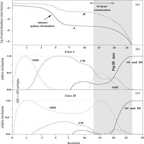
Figure 3: Top: A schematic diagram for the abundance history of the universe. (a) The upper panel shows the global pattern of metal abundances, showing the two major epochs of enrichment of the IGM: first, during the peak of activity of massive Pop III stars around redshift $15-25$ (shaded area), and second, during the peak of galaxy formation around redshift $3-5$ when global rate of star formation reaches maximum. (b) Middle panel shows the relative fraction of three major atomic and ionic species: OI (or HI), CII and OIII, normalized so that the total abundance of all ions of a given element is close to unity at any redshift. The OI abundance closely follows the neutral hydrogen fraction of the universe because their almost similar ionization potential (see discussion in text). The redshift scale is chosen as $log(z+5)$ to emphasize the redshift region $10-30$ of interest to this paper. At very low redshifts ($z<0.7$) the IGM gets heated to very high temperatures ($T\sim 10^{5}-10^{7}$ K) causing even higher ionized species to exist, e.g. OIII $\rightarrow$ OVI. (c) Lower panel shows another variation of relative ion fraction, where Pop III stars ionize all the oxygen around redshift 15, so that OIII have higher abundance and correspondingly OI and CII have lower abundance. Bottom: Frequency dependence of optical depth in atomic and ionic fine-structure lines, in accordance with the abundance history sketched above. Shown here are the contributions from the four most important lines: neutral oxygen $63\mu$, doubly ionized oxygen $88\mu$, singly ionized nitrogen $205\mu$ and singly ionized carbon $158\mu$, and their total contribution for each histories. History of NII ion is taken as similar to that of CII ion.

\psfrag{tempanisotropy}{$l(l+1)/2\pi\ |\delta C_{l}|$ \ \ ($\mu$K${}^{2}$)}\psfrag{123456789empty}{}\psfrag{obsfrequency}{$\nu_{obs}$ \ \ (GHz)}\includegraphics[width=256.0748pt,height=184.9429pt]{contrib_dcl_hisBi.eps}

\psfrag{tempanisotropy}{$l(l+1)/2\pi\ |\delta C_{l}|$ \ \ ($\mu$K${}^{2}$)}\psfrag{123456789empty}{}\psfrag{obsfrequency}{$\nu_{obs}$ \ \ (GHz)}\includegraphics[width=256.0748pt,height=184.9429pt]{contrib_dcl_hisBii.eps}

Figure 4: Frequency dependence of temperature anisotropy generated by scattering from fine-structure lines. We take two ionization histories and the high abundance case from figure (3), and show the contributions of different lines in different frequency range, for a fixed multipole $l=10$. Four different redshift ranges are marked for each species to emphasize the epochs where the dominant contribution from each lines are coming. The sensitivity limits of Planck HFI channels are marked by the crosses. The HFI limits have been improved by a factor of $\sqrt{\Delta l}$ by averaging over in the multipole range $l=7-16$ . The sensitivity limits are for 3 standard deviation detection, and the y-errorbars correspond to $1\sigma$ error in $3\sigma$ detection (we recall that $\sigma=3\sqrt{\sigma_{C_{l}(probe)}^{2}+\sigma_{C_{l}(ref)}^{2}}$, where the reference channel is fixed at HFI 100GHz). The x-errorbars corresponds to the wide bandwidth ($\sim$25%) of Planck HFI channels.

In Fig.3b and 3c , we sketch the relative ion fraction of the three most important atomic and ionic species under above-mentioned ionization history. We show two different reionization scenario: one for relatively cold stars when production OIII is less efficient (case I), and the other for hot stars and quasars which are able to keep oxygen fully ionized at all intermediate redshifts (case II). Line of OI should give us an information about creation of oxygen before Universe was strongly ionised. Relative growth of CII line (see Fig.2b) will mark the time when carbon will be ionised in large ionised regions which do not completely overlap or will be partially ionised everywhere (we can not dinstinguish this two variants of ionization history using large angle observations). Potential of CI ionization (I=11.26 eV) is lower than that of HI. Therefore CII fraction might be higher than that of HII and OII in the beginning of secondary ionization. At the same time OI fraction should follow that of HI because ionization potentials are so close (I=13.62 and 13.60 eV correspondently). Pop III stars should be very hot, and therefore they are able to ionize helium early enough. Simultaneously OIII should become abundant ion because ionization potential of OII (I= 35.12 eV) is higher than that of HeI but smaller then that of HeII.

\psfrag{tempanisotropy}{$l(l+1)/2\pi\ |\delta C_{l}|$ \ \ ($\mu$K${}^{2}$)}\psfrag{multipole}{multipole, $l$}\includegraphics[width=241.84842pt,height=170.71652pt]{car_deviation_1.eps}

Figure 5: Angular dependence of temperature anisotropy generated by scattering from CII 158$\mu$ fine-structure line. Shown here are three cases of $\left|\delta C_{l}\right|$ as should be observed from Planck HFI 143 GHz (scattering at $z=12$), 217 GHz (scattering at $z=8$) and 353 GHz (scattering at $z=4$) channels, (using 100 GHz channel as reference)for 10% abundance of CII ions (with respect to solar) at all three redshifts. Also shown are the primary anisotropy, $C_{l}$, the cosmic variance limit, and noise level for 217 GHz channel (with respect to 100 GHz) for comparison.

\psfrag{temperatureanisotropy}{$l(l+1)/2\pi\ |\delta C_{l}|$ \ \ ($\mu$K${}^{2}$)}\psfrag{obsfrequency}{$\nu_{obs}$ \ \ (GHz)}\includegraphics[width=227.62204pt,height=142.26378pt]{delcl_10_hisABi.eps}

\psfrag{temperatureanisotropy}{$l(l+1)/2\pi\ |\delta C_{l}|$ \ \ ($\mu$K${}^{2}$)}\psfrag{obsfrequency}{$\nu_{obs}$ \ \ (GHz)}\includegraphics[width=227.62204pt,height=142.26378pt]{delcl_10_hisABii.eps}

\psfrag{temperatureanisotropy}{$l(l+1)/2\pi\ |\delta C_{l}|$ \ \ ($\mu$K${}^{2}$)}\psfrag{obsfrequency}{$\nu_{obs}$ \ \ (GHz)}\includegraphics[width=227.62204pt,height=142.26378pt]{hil220_delcl_caseI.eps}

\psfrag{temperatureanisotropy}{$l(l+1)/2\pi\ |\delta C_{l}|$ \ \ ($\mu$K${}^{2}$)}\psfrag{obsfrequency}{$\nu_{obs}$ \ \ (GHz)}\includegraphics[width=227.62204pt,height=142.26378pt]{hil220_delcl_caseII.eps}

\psfrag{temperatureanisotropy}{$l(l+1)/2\pi\ |\delta C_{l}|$ \ \ ($\mu$K${}^{2}$)}\psfrag{obsfrequency}{$\nu_{obs}$ \ \ (GHz)}\includegraphics[width=227.62204pt,height=142.26378pt]{hil810_delcl_caseI.eps}

\psfrag{temperatureanisotropy}{$l(l+1)/2\pi\ |\delta C_{l}|$ \ \ ($\mu$K${}^{2}$)}\psfrag{obsfrequency}{$\nu_{obs}$ \ \ (GHz)}\includegraphics[width=227.62204pt,height=142.26378pt]{hil810_delcl_caseII.eps}

Figure 6: Temperature anisotropy generated by atomic and ionic fine structure lines at different frequencies in the case of three angular scales of observation. The figures on left are for Case I of Fig.3, which is for reionization by stars unable to ionize OII. Figures on right are for Case II, which is for reionization by hot stars and quasars and hence have high OIII fraction. Each figure gives the total contribution for both history A and history B. However, the separate contributions from different lines are given for history A only. We present results for three angular scales: $l=10$ (top), $l=220$ (first Doppler peak, in middle), and $l=810$ (third Doppler peak, at bottom). The scattering-generated $\delta C_{l}$-s are proportional to the intrinsic $C_{l}$-s for higher multipoles, but magnitude is slightly less at the position of third peak because of the reduced power in primary spectrum from $l=220$ to $l=810$.

\psfrag{temperatureanisotropy}{$l(l+1)/2\pi\ |\delta C_{l}|$ \ \ ($\mu$K${}^{2}$)}\psfrag{obsfrequency}{$\nu_{obs}$ \ \ (GHz)}\includegraphics[width=213.39566pt,height=170.71652pt]{sloan_history.eps}

\psfrag{temperatureanisotropy}{$l(l+1)/2\pi\ |\delta C_{l}|$ \ \ ($\mu$K${}^{2}$)}\psfrag{obsfrequency}{$\nu_{obs}$ \ \ (GHz)}\includegraphics[width=230.46748pt,height=173.56198pt]{sloan_delcl_10.eps}

\psfrag{temperatureanisotropy}{$l(l+1)/2\pi\ |\delta C_{l}|$ \ \ ($\mu$K${}^{2}$)}\psfrag{obsfrequency}{$\nu_{obs}$ \ \ (GHz)}\includegraphics[width=233.3125pt,height=142.26378pt]{sloan_delcl_220.eps}

\psfrag{temperatureanisotropy}{$l(l+1)/2\pi\ |\delta C_{l}|$ \ \ ($\mu$K${}^{2}$)}\psfrag{obsfrequency}{$\nu_{obs}$ \ \ (GHz)}\includegraphics[width=233.3125pt,height=142.26378pt]{sloan_delcl_810.eps}

Figure 7: Late ionization and enrichment history of the universe. Top, left: Sketch for the abundance history with late reionization, where first metals are produced around $z\sim 10-12$. Top, right: Temperature anisotropy for this abundance history generated at $l=10$. Also shown are the Planck HFI sensitivity, where the noise levels have again been improved by $\sqrt{\Delta l}$ in the multipole range $10-20$. Bottom left and right: Temperature anisotropy for $l=220$ and $l=810$, respectively.

Fig.4 shows the amplitude of the predicted signal as a function of observing frequency, for a fixed angular scale $l=10$. The contributions from four most important lines, viz. CII 158$\mu$, NII $205\mu$, OI 63$\mu$ and OIII 88$\mu$, are shown, along with their sum. We also show four different redshift ranges for each line, which highlights the fact that contributions from CII and NII are higher because their signal is coming from lower redshifts where abundance is higher according to our chosen abundance history. In Fig.5 we show the angular dependence of the temperature anisotropy generated by resonant line scattering for the three important HFI channels. The abundance of CII ion is kept fixed at 10% solar, so that the lower observing frequency (i.e. higher scattering redshift) has a higher value of optical depth in the same line. The left-side of each curve is dominated by Doppler generation of new anisotropy, and hence are positive. The righ-side is dominated by suppression of primordial anisotropy and hence $\delta C_{l}$-s are negative, the discontinuity in each curve shows the interval where $\delta C_{l}$ changes sign. We see at low multipoles both generation and suppression term tend to cancel each other. Especially due to the adoption of WMAP reionization model with high optical depth ($\tau_{reio}=0.17$) in our computations, lines which scatter CMB photons at redshifts $z\lesssim 18$ encounter a high value of visibility function due to reionization, and therefore causes a strong Doppler generation (but negative) in the multipole range $l=20-100$. This is the cause for higher amplitude of the signal at 143 GHz. But at high multipoles $l>100$ the contribution from Doppler generation is negligible, and the signal is simply proportional to the primordial $C_{l}$-s, and the line optical depth, provided $\tau\ll 1$. Hence using data from table(1), and knowing the amplitude of primordial CMB signal, one can immediately predict the amplitude of the effect at small angular scales using formula(13).

Fig.6 summarizes our results for three different angular scales. As explained above, at low multipoles the effect is not proportional to $C_{l}$, as can be seen from the two panels at top. These low multipole results are important for future satellite missions like Planck and CMBPol. In the middle, results for $l=220$ are shown, where effect is already proportional to $C_{l}$. The amplitude of the signal is highest here due to the large amplitude for the $C_{l}$ at the first Doppler peak. At the bottom we give results for the third Doppler peak, or $l=810$, where signal drops by a factor of $2$ from that of $l=220$. However, these angular scales ($\theta\sim 13^{\prime}$) are particularly suitable for future balloon and ground-based experiments with multi-channel narrow-band recievers.

Finally, in Fig.7, we present an alternative ionization and enrichment history of the universe, when there were no production of heavy elements before $z\sim 12$. This is very interesting because, even for such late reionization, if there is moderate enrichment of the IGM around redshift $4-5$, we have the possibility to detect our signal with Planck HFI around $l=10$. The contributions from high energy oxygen lines are reduced because of the absence of metals at high redshift, but long-wavelength lines of CII and NII still can generate strong signal from low redshifts ($z\lesssim 8$). The HFI sensitivities in this figure have again been improved by averaging the noise in a multipole range of $\Delta l=10$ around $l=10$. As discussed before, the signal for $l=220$ and $l=810$ are proportional to the optical depths in these lines and the primordial $C_{l}$-s.

Due to relatively small scattering cross-sections of the fine-structure transitions under discussion, such observations are sensitive to significant abundances of the atoms and ions (for example when given species contributes from 10% up to 100% of the corresponding element abundance), whereas the Gunn-Peterson effect gives optical depth of the order of unity already when abundance of neutral hydrogen is of the order of $10^{-5}-10^{-6}$. Hence even if the universe is completely opaque to Ly-$\alpha$ photons at redshifts $z\gtrsim 6$, ionic fine-structure lines like CII $157.7\mu$ can probe the very first stages of patchy reionization process. Detection of all three broad spectral features connected with strongly redshifted OI, CII and OIII microwave lines will open the possibility to trace the complete reionization history of the Universe. In addition OIII line will proof the existence of extremely hot stars at that epoch.

The published level of noise of the Planck HFI shows that the three low frequency channels of HFI are almost an order of magnitude more sensitive than signal coming from cases I & II of history B. Even in the case of late reionization history (case C, Fig.7 ), Planck is about 4-times more sensitive than predicted signal. However, to be able to find contribution from at least three lines simultaneously we need higher amount of frequency channels than Planck HFI will have. A higher amount of frequency channels would certainly be possible for the next generation experiments like CMBPol even if they are based on already existing technology (Church 2002).

There is the possibility that balloon and ground-based experiments will be able to check the level of enrichment of the universe by heavy elements even before Planck, observing at $l=220$ and $l=810$, for instance. At these high multipoles, effect is directly proportional to the optical depths in lines and the primordial CMB anisotropy. Hence using the data from table 1 and Fig.3 (bottom), and the simple analytic relation $\delta C_{l}\simeq-2\ \tau_{X_{i}}\ C_{l}^{primary}$, one can immediately give the effect in a first approximation. The high signal-to-noise ratio of the primordial $C_{l}$-s around the first three Doppler peaks will correspondingly give rise to strong signals in scattering, and might become accessible through the tremendous sensitivity promised from the forthcoming balloon and ground-based telescopes like Boomerang, ACT, APEX and SPT.

CBI, VSA and BIMA interferometrs are studying successfully CNB angular fluctuations at low frequencies 30 GHz, there are plans to continue observations on 45, 70 GHz, 90, 100 and 150 GHZ. CI lines with lambda 609 and 370 micron coming from high redshifts 10-15 might contribute to the observed signal at low frequencies.

Beginning of the end of 60-ties theorists are discussing early star formation due to isothermal perturbations, making possible production of heavy elements at redshifts well above 100. This makes interesting the lines with much shorter wavelengths, like $12.8\mu$ Ne II line and many others, which might be contributing to the Planck HFI spectral bands even from redshifts $\sim 100$.

5 Effect of Foregrounds

Before WMAP, the amplitude and spatial and frequency scaling of foregrounds had not been firmly established, and its modeling was merely in a preliminary phase. After their first mission year, WMAP’s team have come up with a foreground model which is claimed to reproduce with a few percent accuracy the observed foreground emission (Bennett et al. 2003b). This and other future studies of foregrounds may provide a characterization of these contaminants such that their effect on our method can be minimized. We next proceed to estimate the impact of these contaminants on our method by the use of current foregrounds models.

Figure 8: (a) Example of optical depth due to a resonant transition which can be detected by the HFI 100 GHz and HFI 143 GHz PLANCK channels in the absence of foregrounds. The upper thick solid line gives the reference model CMB power spectrum. Diamonds show the expected difference in the power spectrum from both channels due to the resonant scattering placed at $z=25$ with $\tau=1\times 10^{-5}$. (b) Presence of foreground contamination after subtracting HFI 100GHz channel from HFI 143GHz channel. The reference $\Lambda$CDM CMB power spectrum is shown in thick solid line, whereas the instrumental noise after the map subtraction is shown in solid intermediate-thickness line. All thin lines refer to the foreground model as quoted as in T00: vibrating dust emission is shown by a dashed line, whereas free-free and synchrotron are given by a dotted and a solid thin line respectively. tSZ effect associated to filaments and superclusters is given by the triple-dot-dashed line. Rotating dust gives negligible contribution at these frequencies. Rayleigh scattering introduces some frequency-dependent variations in the $C_{l}$’s, but well below the noise level (thick dashed line at the bottom right corner). Diamonds show the amplitude of the change in the CMB power spectra induced by resonant species placed at $z=25$ and $\tau=3\times 10^{-4}$.

We have adopted the middle-of-the-road model of Tegmark et al. 2000 (hereafter T00). This model studies separately the contribution coming from different components, giving similar amplitudes for those which are also modelled by the WMAP’s team, (Bennett et al. 2003b). In this model, we will consider the contribution of five foreground sources, namely synchrotron radiation, free-free emission, dust emission, tSZ effect (Sunyaev & Zel’dovich 1972) associated to filaments and superclusters of galaxies, and Rayleigh scattering. The $l$-dependence of the power spectra was approximated by a power law for all foreground components, (except for tSZ, for which the model was slightly more sophisticated). The frequency dependence observed the physical mechanism behind each contaminant: simple power laws were adopted for free-free and synchrotron, whereas a modified black body spectrum was used for dust. For tSZ, the frequency dependence of temperature anisotropies is well known in the non-relativistic regime. All details about this modeling can be found at T00. We are neglecting the contribution from the SZ effect generated in resolved clusters of galaxies which can be removed from the map. We are also assuming that all resolved point sources are excised from the map, and that the contribution from the remaining unresolved point sources ($\sigma_{ps}$ in eq.(10) of T00) can be lowered down to roughly the noise level. This may require the presence of an external point-source catalogue.

Fig.8a shows the expected precision level when foreground contaminations can be neglected, and Fig.8b shows the effect of foregrounds in our differential method to detect the presence of resonant species. Together with the power spectrum of our Standard $\Lambda$CDM model, (thick solid line at the top), we show the contribution from residuals of all foregrounds components under consideration, obtained after subtracting the HFI 100 GHz channel power spectra from the HFI 143 GHz one. The thin solid line corresponds to synchrotron emission, free-free emission is given by the dotted line; the dashed line gives the contribution of dust through vibrational transitions. The tSZ associated to filaments is shown by the triple-dot-dashed line, and the contribution from the combined noise of both channels is shown by the solid line of intermediate thickness which crosses the plot from the bottom left to (almost) the top right corners. At these frequencies, the contribution of rotating dust is negligible, and the most limiting foreground is dust emission by means of vibrational transitions. Finally, the last frequency dependent contribution that we have considered corresponds to Rayleigh scattering. As shown in Yu, Spergel & Ostriker 2001, hereafter YSO, Rayleigh scattering of CMB photons with neutral Hydrogen atoms introduce frequency dependent temperature fluctuations. However, provided that $\tau_{Rayleigh}\propto\nu^{4}$, this process is only effective at high frequencies ($\nu\gtrsim 300$GHz), causing deviations of measured power spectrum from the model $C_{l}$’s of the order of a few percent. YSO characterized the Rayleigh scattering by introducing in the CMBFAST code a frequency dependent effective optical depth and a frequency integrated drag force exerted on the baryons. This last modification, which was neglected when considering resonant scattering, couples the evolution of the different temperature multipoles ($\Delta_{T,l}$) for different frequencies. However, this coupling is exclusively due to the dipole term $\Delta_{T,1}$, which, at the light of their results, is very similar for all frequencies. Taking the same dipole term for every frequency allows us evolving a separate system of differential equation for each frequency. The frequency dependent changes in the angular power spectrum, ($\delta C_{l}/C_{l}(\nu)$), obtained under this approximation are almost identical to those in YSO. For each channel pair under consideration, we computed the residual in the power spectrum difference due to these frequency dependence temperature anisotropies. We checked that this effect was always subdominant. In Fig.8b, the impact of Rayleigh scattering is shown by a middle thick dashed line at the bottom-right corner of the panel, for the particular comparison of the 100GHz and 143GHz channels.

The addition of all contaminants (foregrounds + noise) is given by squares. Diamonds show the change in the power spectrum associated to a resonant transition placed at $z=25$ for optical depth $\tau=3\times 10^{-4}$. After comparing with Fig.8a we can appreciate how the presence of foregrounds affects our method in two different ways: a) it increases the minimum $\tau$ to which the method is sensitive by about two orders of magnitude, b) it changes the range of multipoles to look at, due mainly to the large typical angular size of dust clouds. In the particular case of HFI 100GHz-143GHz channels, one should focus on the range $l\in[100,200]$ once the dust component is included rather than in $l\in[3,10]$ for the foreground-free case. Recurring again to the linear dependence of $\tau$ versus the abundance, eq.(4), we see that this model of foregrounds increases by about two orders of magnitude the minimum abundance on which future CMB missions will be able to put constraints.

6 Conclusions

In this paper, we have computed the effect of heavy elements on the Cosmic Microwave Background. We have selected those species which might leave a greater signature in the CMB power spectrum, and analyzed the possibility of constraining their abundances by the use of forthcoming CMB data.

Under the approximation of negligible drag force, we have computed what are the changes in the CMB angular power spectra introduced by resonant species placed at redshifts which are dependent on the observing and resonant frequencies. The overall effect can be decomposed into a damping or suppression of the original CMB temperature fluctuations, and a generation of new anisotropies. For the optically thin limit to which we have restricted ourselves, damping dominates over generation of new anisotropies in the intermediate and high multipole range ($l\gtrsim 20$).

These changes in the CMB are of very small amplitude ($0.01-0.3\mu K$), and could be distinguished from the CMB component by means of their frequency dependence. Indeed, a comparison with respect to a reference channel containing only non-frequency dependent temperature fluctuations could be used to quantify the amount of angular power introduced by the resonant species. However, this would only be feasible if either the other frequency-dependent components are negligible or characterized with extreme accuracy. The possible presence of foregrounds, galactic of extragalactic, whose amplitude and spectral behavior is still under characterization, is a serious aspect to be taken into account. Other technical challenges, such as the calibration of different channels and the enormous sensitivity required, should be accessible from the next generation of detector technology.

We have obtained limits for abundances of heavy elements when complete foreground removal is possible, but also have shown values when all foregrounds are present in the sky map. Our analyses have particularly focused on PLANCK HFI channels, whose very low noise levels give extremely strong limits on abundances. It is easiest to observe the proposed effect with HFI at angular scales of $\theta\sim 20^{\circ}$ or $l\sim 10$ because of the very low noise of the first three HFI channels at these multipoles. Using the 143 & 217 GHz channels of HFI, with the 100 GHz channel as reference, limits as low as $10^{-3}-10^{-4}$ solar abundance were obtained for atoms and ions of the most important elements like carbon, nitrogen and oxygen in the redshift range $[5,30]$. At higher multipoles ($l>200$), we have shown that future balloon and ground-based experiments like ACT, APEX and SPT can put similar constraint on abundances, where the predicted signal is stronger because of the higher amplitude of the primordial CMB signal, and effect will be directly proportinal to the optical depths in lines. The presence of foregrounds makes all these limits about a factor of $10^{2}$ worse, but that must be considered as the most pessimistic scenario.

In this paper we have considered scattering of CMB photons by low density gas everywhere in the universe, where optical depths in the relevant atomic or molecular lines are very low and resonant scattering effect dominates over line emission. The effect connected with scattering from atomic and ionic fine-structure transitions depends on the amount of of atoms/ions in the ground state, which is determined by the excitation temperature. In Appendix B we showed that even up to very high over-density of the plasma, the change in excitation temperature from the CMB temperature is negligible, and our simple approximation is valid. The clustering of heavy atoms and molecules in clouds should change the predictions on the modifications of the CMB power spectrum at smaller angular scales, and will be discussed in a subsequent work.

Appendix A

METHOD OF COMPUTATION:

Our approach to model the coupling between these heavy species and CMB photons will be similar to that outlined in Zaldarriaga & Loeb (2002, ZL02). In their paper they discussed modifications of CMB spectrum by presence of primordial Lithium atoms. Here we extend their analysis to other atoms and ions. We also discuss the necessary changes that are enforced while extending this method to all resonant species.

As a first step, we describe the modifications introduced in the CMBFast code in order to compute the effect of resonant transitions. We consider a given resonant transition i of a given species X, with a resonant frequency $\nu_{X_{i}}$. For a fixed observing frequency $\nu_{obs}$, the redshift at which that species interacts with the CMB is $1+z=\nu_{X_{i}}/\nu_{obs}$, and its opacity can be written, in general, as $\dot{\tau}_{X_{i}}=\tau_{X_{i}}{\cal P}(\eta)$, with a normalized profile function $\int_{0}^{\eta_{0}}d\eta^{\prime}{\cal P(\eta^{\prime})}=1$. We shall model this profile with a gaussian:

$$\dot{\tau}_{X_{i}}=\tau_{X_{i}}\;\frac{\exp{\left(-\frac{\left(\eta-\eta_{X_{i}}\right)^{2}}{2\sigma_{X_{i}}^{2}}\right)}}{\sqrt{2\pi\sigma_{X_{i}}^{2}}}$$ (17)

where $\tau_{X_{i}}$ is the optical depth for the specific transition, $\eta_{X_{i}}$ is the conformal time corresponding to the redshift $1+z_{X_{i}}=\nu_{X_{i}}/\nu_{obs}$ where scattering takes place, and $\sigma_{X_{i}}$ is the width of the gaussian. For a fixed transition, this width should be given by the thermal broadening of the line. For the sake of simplicity, we shall take $\sigma_{X_{i}}\sim 0.01\eta_{X_{i}}$.

Once the line optical depth has been characterized, (as shown in Section 2), the new opacity term with a gaussian profile is added to the standard Thompson opacity,

$$\dot{\tau}=an_{e}\sigma_{T}+\sum_{i}\tau_{X_{i}}\frac{\exp{\left(-\frac{\left(\eta-\eta_{X_{i}}\right)^{2}}{2\sigma_{\eta_{X_{i}}}^{2}}\right)}}{\sqrt{2\pi\sigma_{\eta_{X_{i}}}^{2}}},$$ (18)

and this in turn is used to compute the visibility function $\Upsilon(\eta)$, defined as

$$\Upsilon(\eta)={\dot{\tau}}(\eta)e^{-\tau(\eta)}.$$ (19)

This scattering introduces a frequency dependent term in the evolution equation for the photon distribution function, which results in a frequency dependence drag-force. However, based on the same arguments of ZL02 , we can safely ignore this drag-force as long as the characteristic time of drag exerted by these species is far larger than the Hubble time, which is indeed the case due to the low optical depths under consideration. These are the modifications we introduced in the CMBFAST code in order to compute the CMB power spectrum under the presence of scattering by atoms and ions.

ANALYTICAL FORM OF $\delta C_{l}$’s:

Following eq.(7) for the k-mode of the photon temperature fluctuation,

$$\Delta_{T}(k,\eta_{0},\mu)=\int_{0}^{\eta_{0}}d\eta\;e^{ik\mu(\eta-\eta_{0})}\ \$$

$$\phantom{xxxxxxxxxxxxx}\times\ \bigl{[}\Upsilon(\eta)\left(\Delta_{T0}-i\mu v_{b}\right)+\dot{\phi}+\psi-ik\mu\psi\bigr{]},$$ (20)

we proceed now to characterize the change in the radiation power spectrum. In eq.(20), the terms in the angle $\mu=\bf{\hat{k}}\cdot{\bf{\hat{n}}}$ can be eliminated after integrating by parts and neglecting the contribution of boundary terms, (Seljak & Zaldarriaga 1996). This gives:

$$\Delta_{T}=\int_{0}^{\eta_{0}}d\eta\;e^{ik\mu(\eta-\eta_{0})}S(k,\eta),$$ (21)

where the source term $S(k,\eta)$ is defined as

$$S(k,\eta)=e^{-\tau}\left(\dot{\phi}+\dot{\psi}\right)+\Upsilon\left(\Delta_{T0}+\psi+\frac{\dot{v_{b}}}{k}\right)+\dot{\Upsilon}\left(\frac{v_{b}}{k}\right).$$ (22)

From this source term, the angular power spectrum can be expressed as, (e.g. Seljak & Zaldarriaga, 1996):

$$C_{l}=\left(4\pi\right)^{2}\int dk\;k^{2}P_{\psi}(k)\;\left|\int_{0}^{\eta_{0}}d\eta S(k,\eta)j_{l}\left[k(\eta_{0}-\eta)\right]\right|^{2}$$

$$\phantom{xx}=\left(4\pi\right)^{2}\int dk\;k^{2}P_{\psi}(k)\left|\Delta_{T,l}\right|^{2},$$ (23)

where $j_{l}$ is the spherical Bessel function of order $l$ and $P_{\psi}(k)$ is the initial scalar perturbation power spectrum. If at a given frequency the CMB interacts through the resonant transition $i$ of a species X, the measured power spectrum will differ from the reference one by an amount:

$$\delta C_{l}\equiv C_{l}^{X_{i}}-C_{l}$$

$$\phantom{xx}=(4\pi)^{2}\int dk\;k^{2}P_{\psi}(k)\ \bigl{[}\left|\int_{0}^{\eta_{0}}d\eta\;S^{X_{i}}(k,\eta)j_{l}\left[k\left(\eta_{0}-\eta\right)\right]\right|^{2}$$

$$\phantom{xxxxxxxxxxxx}-\left|\int_{0}^{\eta_{0}}d\eta\;S(k,\eta)j_{l}\left[k(\eta_{0}-\eta)\right]\right|^{2}\bigr{]}\;$$

$$\phantom{xx}=\left(4\pi\right)^{2}\int dk\;k^{2}P_{\psi}(k)\bigl{[}\;\left|\Delta_{T,l}^{X_{i}}\right|^{2}-\left|\Delta_{T,l}\right|^{2}\bigr{]}\;$$

$$\phantom{xx}=\left(4\pi\right)^{2}\int dk\;k^{2}P_{\psi}(k)\bigl{[}2\;\Delta_{T,l}+\delta\Delta_{T,l}\bigr{]}\delta\Delta_{T,l}$$ (24)

with $\delta\Delta_{T,l}\equiv\int_{0}^{\eta_{0}}d\eta\;\left(S^{X_{i}}(k,\eta)-S(k,\eta)\right)j_{l}\left[k(\eta_{0}-\eta)\right]$, and where the term $S^{X_{i}}(k,\eta)$ refers to the sources including the species $X$. Note that the cross term $2\;\Delta_{T,l}\cdot\delta\Delta_{T,l}$ only arises after computing the difference of the power spectra, i.e., it is not present if one computes the power spectrum of the difference of two maps obtained at different frequencies. This cross term is precisely the responsible of having $\delta C_{l}$ linear in $\tau_{x_{i}}$, and hence also linear in the abundance of the species $X_{i}$. This term also accounts for the correlation existing between the temperature fluctuations generated during recombination and those generated during the scattering with the species $X$. This non-zero correlation is essentially due to those $k$ modes corresponding to lengths bigger than the distance separating the two events, i.e., recombination and scattering with $X$, (Hernández-Monteagudo & Sunyaev, in preparation). Let us now model the differential opacity due to this transition as $\dot{\tau_{X_{i}}}=\tau_{X_{i}}{\cal P}(\eta)$, where ${\cal P}(\eta)$ is a profile function of area unity, $\int_{0}^{\eta_{0}}d\eta^{\prime}\;{\cal P}(\eta^{\prime})=1$. We write the optical depth as $\tau_{tot}(\eta)=\tau(\eta)+\tau_{X_{i}}(\eta)$, where the last term refers to the optical depth due to the transition $i$ of the X species. It can be expressed as $\tau_{X_{i}}(\eta)=\tau_{X_{i}}\;{\cal A}(\eta)=\tau_{X_{i}}\int_{\eta}^{\eta_{0}}d\eta^{\prime}\;{\cal P}(\eta^{\prime})$, with ${\cal A}(\eta)$ the area function of the profile ${\cal P}(\eta)$. We will assume that the profile peaks at $\eta=\eta_{X_{i}}$ and that $\eta_{-}$ and $\eta_{+}$ are such that ${\cal P}(\eta)\approx 0$ for $\eta<\eta_{-}$ and $\eta>\eta_{+}$. Hereafter, $\eta_{X_{i}}$ will be referred to as transition epoch or line epoch. If we add this new term to the opacity, and assume that $\tau_{X_{i}}\ll 1$, then we can expand the term $\delta\Delta_{T,l}$ in a power series of $\tau_{X_{i}}$. In this case, we obtain:

$$\delta\Delta_{T,l}\ =\ \tau_{X_{i}}\cdot\biggl{\{}-\int_{0}^{\eta_{+}}d\eta\;j_{l}\left[k(\eta_{0}-\eta)\right]{\cal A}(\eta)$$

$$\phantom{xxxx}\times\ \left[e^{-\tau}\left(\dot{\phi}+\dot{\psi}\right)+\dot{\tau}e^{-\tau}\left(\Delta_{T0}+\psi+\frac{\dot{v_{b}}}{k}\right)+\;e^{-\tau}\left(\ddot{\tau}+\dot{\tau}^{2}\right)\frac{v_{b}}{k}\right]$$

$$\phantom{xxxxxxx}+\ \int_{0}^{\eta_{+}}d\eta\;j_{l}\left[k(\eta_{0}-\eta)\right]{\cal P}(\eta)e^{-\tau}$$

$$\phantom{xxxxxxxxxxxxx}\times\ \left[\left(\Delta_{T0}+\psi+\frac{\dot{v_{b}}}{k}\right)+\left(\frac{1}{{\cal P}}\frac{d{\cal P}}{d\eta}+2\dot{\tau}\right)\frac{v_{b}}{k}\right]\biggr{\}}$$

$$\phantom{xxxx}+\ \ \tau_{X_{i}}^{2}\cdot\biggl{\{}\frac{1}{2}\int_{0}^{\eta_{+}}d\eta\;j_{l}\left[k\left(\eta_{0}-\eta\right)\right]{\cal A}^{2}(\eta)$$

$$\phantom{xxxxx}\times\ \biggl{[}e^{-\tau}\left(\dot{\phi}+\dot{\psi}\right)+\dot{\tau}e^{-\tau}\left(\Delta_{T0}+\psi+\frac{\dot{v_{b}}}{k}\right)+\ e^{-\tau}\left(\ddot{\tau}+\dot{\tau}^{2}\right)\frac{v_{b}}{k}\;\;\biggr{]}$$

$$\phantom{xxxxxxxxxx}+\ \int_{0}^{\eta_{+}}d\eta\;j_{l}\left[k\left(\eta_{0}-\eta\right)\right]e^{-\tau}\;\times$$

$$\phantom{xxxxxxxxxxxxxxxxx}\biggl{[}-\left(\Delta_{T0}+\psi+\frac{\dot{v_{b}}}{k}\right){\cal A}(\eta){\cal P}(\eta)$$

$$\phantom{xxxxxxxxxxxxxxxxxxx}\times\ \frac{v_{b}}{k}\left({\cal P}^{2}(\eta)+{\cal A}(\eta)\left(-\frac{d{\cal P}}{d\eta}-2\dot{\tau}\right)\right)\biggr{]}\biggr{\}}$$

$$\phantom{xxxx}+\;\phantom{x}{\cal O}(\tau_{X_{i}}^{3})\;$$

$$\phantom{xxxx}=\tau_{X_{i}}\cdot{\cal D}_{1}+\tau_{X_{i}}^{2}\cdot{\cal D}_{2}+{\cal O}(\tau_{X_{i}}^{3}).$$ (25)

It is worth to note that ${\cal D}_{1}$ contains both the suppression of intrinsic CMB anisotropies, and the generation of new fluctuations at line epoch. This expansion allows us writing $\delta C_{l}$ as a power series of $\tau_{X_{i}}$ as well,

$$\delta C_{l}\;=\phantom{x}\tau_{X_{i}}\cdot(4\pi)^{2}\int dk\;k^{2}P_{\psi}(k)\left[{\cal D}_{1}\;2\Delta_{T,l}\right]$$

$$\phantom{xxxx}+\;\tau_{X_{i}}^{2}\cdot(4\pi)^{2}\int dk\;k^{2}P_{\psi}(k)\left[{\cal D}_{2}\;2\Delta_{T,l}+{\cal D}_{2}^{2}\right]$$

$$\phantom{xxxx}+\;{\cal O}(\tau_{X_{i}}^{3})$$

$$\phantom{xxxx}=\;\tau_{X_{i}}\cdot{\cal C}_{1}+\tau_{X_{i}}^{2}\cdot{\cal C}_{2}+{\cal O}(\tau_{X_{i}}^{3})$$ (26)

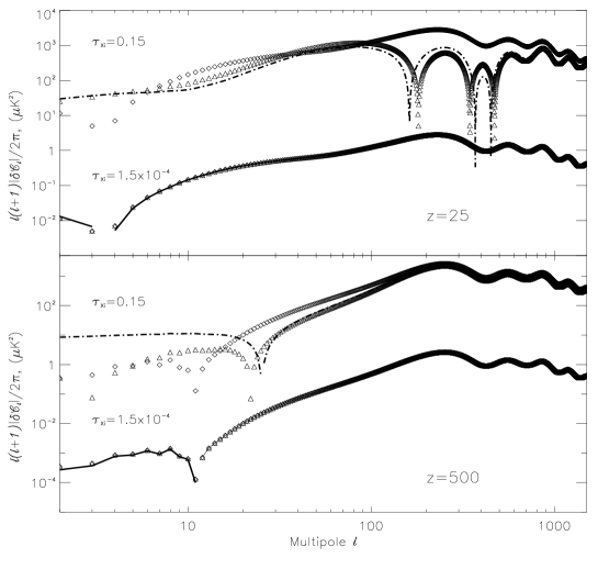
Figure 9: This figure shows the validity of the linear (diamonds) and quadratic (triangles) approximations on $\tau$ when trying to describe the changes induced in the power spectrum by a resonant transition ($\delta C_{l}$’s). We see that both suffice to accurately match the theoretical $\delta C_{l}$’s for redshifts 25 (top panel) and 500 (bottom panel) and for $\tau=1.5\times 10^{-4}$, (solid lines). However, when $\tau$ is closer to one (dot-dashed lines), the quadratic approximation performs remarkably better than the linear one.

Figure 10: Study of the different contributions to ${\cal C}_{1}$ in eq.(12). Diamonds give ${\cal C}_{1}$ versus multipole. We are plotting only absolute values. In units of $\tau_{X_{i}}$, we plot the damping term in solid line. The term responsible for the generation of new anisotropies is plotted in thick dashed line. Its two components, monopole ($(\Delta_{0}+\psi)$) and velocity, are also displayed in thin dashed and thin dotted lines respectively. As conformal time goes by, the relative weight of the velocity term with respect the monopole term increases, and the sum of both at low multipoles approaches the amplitude of the original CMB anisotropies, (solid line). Both generation and damping tend to cancel each other at a multipole $l=l_{X_{i}}$, dependent on the epoch of interaction $\eta_{X_{i}}$.

The result of this expansion is displayed in Fig.9: the change in the power spectrum induced by resonant transitions is computed for different redshifts, 25 (top panel) and 500 (bottom panel), and different amplitudes of the optical depth (solid lines correspond to $\tau=1.5\times 10^{-4}$ and dot-dashed lines to $\tau=0.15$). Diamonds give the linear approximation in $\tau$, whereas triangles show the quadratic one. Both match the exact $\delta C_{l}$’s fairly well for the low $\tau$ cases. Therefore, by means of eq.(4), we can establish a linear relation between $\delta C_{l}$ and the abundance of the species.

In Fig.10, diamonds show the absolute value of ${\cal C}_{1}$ versus $l$. As shown above, this term is the sum of two integrals. The first one is the suppression induced by the $e^{-\tau_{X_{i}}}$ term, (thick solid line in the figure), whereas the second contain the newly generated anisotropies, (thick dashed line). The latter term has a monopole ($\Delta_{0}+\psi$, thin dashed line) and a velocity (thin dotted line) contribution. We are plotting absolute values of all terms. As pointed out by ZL02, the monopole term decreases with cosmic time and hence the velocity term becomes the most important source of generation of new anisotropies. However, this generation takes place at the transition epoch, and hence is shifted towards the low multipole range. It is easy to show that the maximum multipole below which generation becomes significant is roughly given by $l_{X_{i}}\sim 2\pi\;\left(\eta_{0}-\eta_{X_{i}}\right)/\eta_{X_{i}}$. We show that the suppression term is dominant for high multipoles, and only at very low multipoles suppression and generation tend to cancel each other. Only if higher orders in the power expansion are relevant, (i.e., if $\tau_{X_{i}}\sim 1$) the newly generated anisotropies become important.

This cancellation of suppression and generation terms at low multipoles can be better understood when coming back onto eq.20. If in this equation we substitute $\tau$ by $\tau+\tau_{X_{i}}$, we find that the change in the temperature modes due to $\tau_{X_{i}}$ can be written as:

$$\delta\Delta_{T}=\;\left(e^{-\tau_{X_{i}}}-1\right)\;\int_{0}^{\eta_{0}}\;d\eta\;e^{ik\mu(\eta-\eta_{0})}\dot{\tau}e^{-\tau}\left(\Delta_{T0}-i\mu v_{b}\right)$$

$$\phantom{xxxxx}+\;e^{-\tau_{X_{i}}}\;\int_{0}^{\eta_{0}}\;d\eta\;e^{ik\mu(\eta-\eta_{0})}\dot{\tau}_{X_{i}}e^{-\tau}\left(\Delta_{T0}-i\mu v_{b}\right),$$ (27)

where we have applied the definition of the visibility function, $\Upsilon(\eta)=\dot{\tau}(\eta)\;e^{-\tau(\eta)}$. However, recalling that the visibility function gives the probability of a photon being emitted at a given $\eta$, and taking $\dot{\tau}_{X_{i}}=\tau_{X_{i}}\delta_{D}(\eta-\eta_{X_{i}})$, the last equation merely implies that

$$\delta\Delta_{T}\simeq\tau_{X_{i}}\left[\Delta_{T0}(\eta_{X_{i}})-\Delta_{T0}(\eta_{rec})-i\mu\left(v_{b}(\eta_{X_{i}})-v_{b}(\eta_{rec})\right)\right],$$ (28)

where we have taken into account that $\tau_{X_{i}}$ is much smaller than unity, and approximated the exponentials to unity, as we shall focus on the very low $k$ range. That is, the change in the temperature mode $\Delta_{T}(k,\mu,\eta)$ reflects the difference of the monopole ($\Delta_{T0}$) and velocity terms when evaluated at recombination and at the transition epochs. We can estimate how this difference projects onto multipole space if we restrict ourselves to the low multipole (large angle) range. For the scattering redshifts under consideration ($z_{X_{i}}>$ a few), we can safely neglect the term due to the Integrated Sachs-Wolfe effect. Then from eq.(20), one finds that the time dependence of the monopole term $\Delta_{T0}(\eta)$ can be approximated as $\Delta_{T0}(\eta)\simeq\Delta_{T0}(\eta_{rec})\;j_{0}\left(k\left[\eta-\eta_{rec}\right]\right)$, where $j_{0}(x)$ is the spherical Bessel function of order zero. From this dependence, it is easy to see that at low multipoles, i.e., at small enough $k$’s, $\Delta_{T0}(\eta_{rec})$ and $\Delta_{T0}(\eta_{\eta_{X_{i}}})$ will be roughly equal, and thus their difference in the equation above will tend to vanish. This can also be seen in Fig.10, where the contribution of the monopole term to ${\cal C}_{1}$ (thin dashed line) has roughly the same amplitude at redshifts 500 and 25 for $l<10$. This behaviour is the responsible for the cancellation of the $\delta C_{l}$’s at low $l$’s. In this situation, the difference of the velocity terms will be of particular relevance. The evolution of velocities can be approximated, after integrating in $\mu$, as $v_{b}(\eta)\simeq v_{b}(\eta_{rec})\dot{D}(\eta)/\dot{D}(\eta_{rec})j_{1}\left(k\left[\eta-\eta_{rec}\right]\right)$, with $D(\eta)$ the linear growth factor . The growth of velocities will assure an increase of the Doppler-induced anisotropy power. Finally, due to the fact that $j_{l}(x)$ is maximum at $x\sim l$, then we have that the Doppler term will predominantly contribute for $k\sim 2\pi/\eta_{X_{i}}$, which corresponds to multipoles $l_{X_{i}}\sim 2\pi\left(\eta_{0}-\eta_{x_{i}}\right)/\eta_{X_{i}}$. Again, this can be checked by looking at the velocity term (dotted line) in Fig.10: the power is projected at lower multipoles at later epochs, scales at which the amplitude grows with conformal time as $\dot{D}$.

Therefore, the factors determining the cross-over of the $\delta C_{l}$’s from (Doppler-induced) positive values at small $l$ to (absorption-induced) negative values at large $l$ are two: a) the constant amplitude of the monopole at large scales, and b) the growth of peculiar velocities with cosmic time . The angular scale at which such crossing takes place is roughly determined by the time at scattering epoch, $\eta_{X_{i}}$, $l_{X_{i}}\sim 2\pi\left(\eta_{0}-\eta_{x_{i}}\right)/\eta_{X_{i}}$.

Appendix B

LINE EMISSIVITY:

The volume emissivity for line emission due to collisional excitation can be written as

$$j_{\nu}^{line}={\frac{h\nu}{4\pi}}\ \langle n_{i}\ n_{c}\rangle\ \gamma_{lu}\ \varphi(\nu^{\prime}),$$ (29)

expressed in $erg\ cm^{-3}s^{-1}Hz^{-1}str^{-1}$ in the rest frame of the emitter. Here $n_{i}$ is the number density of the atom or ion under consideration, and $n_{c}$ is the number density of the colliding particle, and $\langle n_{i}\ n_{c}\rangle$ means averaging over the volume specified by multipole $l$, corresponding to the angular size of observation, and the thickness of the slice along the line-of-sight defined by the frequency resolution of the experiment. $h\nu$ is the energy of the emitted photon, $\gamma_{lu}$ is the collision rate-coefficient between between the two levels, and $\varphi(\nu^{\prime})$ is the line-profile function, which we can approximate by a $\delta$-function because experimental bandwidth is much larger than velocity or thermal broadening,

$$\varphi(\nu^{\prime})=\delta(\nu^{\prime}-\nu)={\frac{1+z}{\nu}}\ \delta(z^{\prime}-z)\ ,$$ (30)

where $z$ corresponds to the redshift under study. Eqn.(29) is correct for the low density gas ($n\ll n_{crit}$) that we are concerned with in this paper. This emissivity produces a line flux, written as following in an expanding universe (neglecting absorption because $\tau_{\nu}\ll 1$)

$$F_{\nu}^{line}=\int{\frac{j_{\nu}}{(1+z)^{3}}}\ dl,$$ (31)

where the integration is along the line-of-sight. This creates a distortion in the thermal spectrum of the background CMB photons

$${\frac{\Delta T}{T_{\gamma}}}={\frac{e^{x}-1}{xe^{x}}}\ {\frac{F_{\nu}}{B_{\nu}}}\ ,\ \ \ \ \ \ \ \ \mbox{where}\ \ x\equiv{\frac{h\nu}{kT_{\gamma}}}$$ (32)

with $T_{\gamma}$ as the mean temperature of CMB photons, and $B_{\nu}$ being the Planck function.

EFFECT OF OVER-DENSITY:

In this subchapter, we consider the impact of collisions in our study. Collisions with electrons (or neutral atoms in the case of neutral gas) cause emission from the same atomic and ionic fine-structure lines and hence change the observed $\delta C_{l}$-s by producing an additional and independent signal on the top of the scattering signal.

In addition, collisions are decreasing the population of the ground level in the transitions under consideration, dimishing the optical depth due to scattering in the line. In what follows, we compute the deviation of the equilibrium excitation temperature of a two-level system from the background cosmic microwave radiation temperature as a function of the over-density of the enriched region. we estimate the required over-density for causing a given amount (30% or 50%) decrease in the optical depth.

We consider a two-level system (like CII or NIII ion) for simplicity, whose population ratio between the two levels is determined by the excitation temperature, $T_{EX}$, defined as

$$(n_{u}/n_{l})=(g_{u}/g_{l})\exp\left[-h\nu/kT_{EX}\right]$$ (33)

where $n_{u}$ and $n_{l}$ are the relative fraction of atoms/ions in upper or lower levels, respectively, and $g_{u}$ and $g_{l}$ are the statistical weights of each level. The equilibrium population ratio is obtained by solving the statistical balance equation:

$$n_{u}\left(A_{ul}+B_{ul}J_{\nu}+n_{e}\gamma_{ul}\right)\ =\ n_{l}\left(\frac{g_{u}}{g_{l}}B_{ul}J_{\nu}+\frac{g_{u}}{g_{l}}n_{e}\gamma_{ul}e^{-h\nu/kT_{K}}\right)$$ (34)

Here $A_{ul}$ and $B_{ul}$ are the Einstein coefficients for spontaneous and stimulated emission, and $J_{\nu}$ is the background radiation field of CMB photons, $J_{\nu}\equiv(2h\nu^{3}/c^{2})[\exp(h\nu/kT_{CMB})-1]^{-1}$. $T_{CMB}$ is the radiation temperature at redshift $z$, defined by $T_{CMB}\equiv T_{0}(1+z)$, with $T_{0}=2.726$ K.  $n_{e}$ is the electron density inside the object at redshift $z$ , connected to its over-density $\delta$ by the following: $n_{e}(z)\equiv\bar{n}_{e}(z)\ (1+\delta)$, where $\bar{n}_{e}(z)=2.18\times 10^{-7}(1+z)^{3}$ cm^-3.  $\gamma_{ul}$ is the collisional de-excitation rate (in cm³ s^-1), and $T_{K}$ is the kinetic temperature of the electrons, which we assume to be roughly constant at $10^{4}$ K. Then from eqn.(33) we can express the over-density as a function of excitation temperature:

$$1+\delta=\frac{A_{ul}\left[(1+\Gamma)e^{-h\nu/kT_{EX}}-\Gamma\right]}{\bar{n}_{e}(z)\ \gamma_{ul}\left[e^{-h\nu/kT_{K}}-e^{-h\nu/kT_{EX}}\right]}$$ (35)

where $\Gamma\equiv[\exp(h\nu/kT_{CMB}(z))-1]^{-1}$, and we have used $B_{ul}=(c^{2}/2h\nu^{3})A_{ul}$. Eqn.(35) is exact, which can be further simplified in the limit of low redshifts, when the line is in the Wien part of the CMB spectrum ($T_{CMB}(z)<T_{EX}\ll h\nu$)

$$1+\delta=\frac{A_{ul}\left[e^{-h\nu/kT_{EX}}-e^{-h\nu/kT_{CMB}(z)}\right]}{\bar{n}_{e}(z)\ \gamma_{ul}\left[1-\frac{h\nu}{kT_{K}}-e^{-h\nu/kT_{EX}}\right]}$$ (36)

At $n_{e}<A_{ul}/\gamma_{ul}$ collisions do not influence the population of the ground level because radiative transitions are faster than excitations due to collisions. If density is higher, population of the ground level decreases and optical depth due to resonance scattering drops correspondingly, diminishing the effect we have discussed in this paper.

Figure 11: Over-density and actual electron number density required to cause significant deviation of the excitation temperature from the background cosmic microwave temperature, as function of redshift. Shown here are the cases for CII and NIII fine-structure singlets. The thick lines are for CII ion,and the thin ones are for NIII ions. The pair of solid and dashed lines correspond to 30% and 50% decrease in the optical depth for the same column density, respectively

Obviously, a very large over-density is needed in order to produce any significant amount of deviation from the CMB equilibrium, as can be seen from Fig.11 for the case of CII 158$\mu$ and NIII 57$\mu$ transitions. These two transitions are picked as they both arise from two-level fine-structure splitting, but results are similar for all other relevant atoms and ions. In the bottom panel of Fig.11, we see that the electron density required to cause a given amount of depopulation of the ground level is constant for low redshifts, and this density is less than the critical density for that transition (e.g., with CII 158$\mu$ line, we have $\gamma_{ul}=4.6\times 10^{-8}$ cm³ s^-1 for collision with electrons at $10^{4}$K, and the ratio $A_{ul}/\gamma_{ul}=50$ cm^-3. This simple estimate gives 5-10 times higher critical density than the more exact approach shown in Fig.11). Hence, we conclude that the effectiveness of the resonant scattering process decreases in the most over-dense regions of the universe. Atoms and ions of heavy elements everywhere else including less over-dense halos and clouds participate in the process and contribute into the angular fluctuations of the CMB we discussed in this paper.