Local Supermassive Black Holes, Relics of Active Galactic Nuclei and the X-ray Background
Abstract
We quantify the importance of mass accretion during AGN phases in the growth of supermassive black holes () by comparing the mass function of black holes in the local universe with that expected from AGN relics, which are black holes grown entirely with mass accretion during AGN phases. The local mass function () is estimated by applying the well-known correlations between mass, bulge luminosity and stellar velocity dispersion to galaxy luminosity and velocity functions. We find that different correlations provide the same only if they have the same intrinsic dispersion. The density of supermassive black holes in the local universe which we estimate is . The relic is derived from the continuity equation with the only assumption that AGN activity is due to accretion onto massive ’s and that merging is not important. We find that the relic at is generated mainly at where the major part of ’s growth takes place. Moreover, the growth is anti-hierarchical in the sense that smaller ’s () grow at lower redshifts () with respect to more massive one’s (). Unlike previous work, we find that the of AGN relics is perfectly consistent with the local indicating the local black holes were mainly grown during AGN activity. This agreement is obtained while satisfying, at the same time, the constraints imposed from the X-ray background. The comparison between the local and relic ’s also suggests that the merging process is not important in shaping the relic , at least at low redshifts (), and allows us to estimate the average radiative efficiency (), the ratio between emitted and Eddington luminosity () and the average lifetime of active ’s. Our analysis thus suggests the following scenario: local black holes grew during AGN phases in which accreting matter was converted into radiation with efficiencies and emitted at a fraction of the Eddington luminosity. The average total lifetime of these active phases ranges from yr for to yr for but can become as large as for the lowest acceptable and values.
keywords:
black hole physics - galaxies: active - galaxies: evolution - galaxies: nuclei - quasars: general - cosmology: miscellaneous1 Introduction
Since the discovery of quasars (Schmidt 1963) it has been suggested that Active Galactic Nuclei (AGN) are powered by mass accretion onto a supermassive Black Hole () with mass in the range - (Salpeter 1964; Zel’dovich & Novikov 1964; Lynden-Bell 1969). This paradigm combined with the observed evolution of AGNs implies that a significant number of galaxies in the local universe should host a supermassive (e.g. Sołtan 1982; Cavaliere & Padovani 1989; Chokshi & Turner 1992).
Supermassive ’s are now detected in galaxies through gas and stellar dynamical methods (Kormendy & Gebhardt 2001; Merritt & Ferrarese 2001b). Some galaxies are quiescent (e.g. M32, van der Marel et al. 1997; NGC 3250, Barth et al. 2001) and some are mildly or strongly active (e.g. M87, Marconi et al. 1997; Macchetto et al. 1997; Centaurus A, Marconi et al. 2001; Cygnus A, Tadhunter et al. 2003). The mass of the correlates with some properties of the host galaxy such as spheroid (bulge) luminosity and mass (Kormendy & Richstone 1995; Magorrian et al. 1998), light concentration (Graham et al. 2001) and with the central stellar velocity dispersion (Ferrarese & Merritt 2000; Gebhardt et al. 2000). The latter correlation was thought to be the tightest but Marconi & Hunt (2003) have recently shown that all the correlations have similar intrinsic dispersion when considering only galaxies with secure BH detections (see also McLure & Dunlop 2002; Erwin, Graham, & Caon 2003). Overall, the dispersion is of the order of 0.3 in at a given value of , or . The existence of any correlations of and host galaxy bulge properties has important implications for theories of galaxy formation in general and bulge formation in particular. Indeed, several attempts at explaining the origin of these correlations and the difficulties/constraints that they pose to galaxy formation models can be found in the literature (e.g. Silk & Rees 1998; Cattaneo, Haehnelt, & Rees 1999; Haehnelt & Kauffmann 2000; Ciotti & van Albada 2001; Cavaliere & Vittorini 2002; Adams et al. 2003, and references therein).
To date, all newly found ’s have masses (or upper limits) in agreement with those expected from the above correlations suggesting that all galaxies host a massive in their nuclei. By applying the correlations between and host galaxy properties it is then possible to estimate the mass function of local ’s or, more simply, their total mass density () in the local universe (e.g. Salucci et al. 1999; Marconi & Salvati 2002; Yu & Tremaine 2002; Ferrarese 2002; Aller & Richstone 2002).
It is important to verify if local BH’s are exclusively relics of AGN activity or if other mechanisms, such as merging, play a role. Hereafter we will call ’AGN relics’, or simply relics, those black holes which grew up from small seeds (1-) following mass accretion during AGN phases. For instance, an AGN relic of is different from a of the same mass but which was formed by the merging of many smaller ’s.
A simple comparison between local and relic BH’s was performed by Salucci et al. (1999) and Fabian & Iwasawa (1999) who determined from the observed X-ray background emission. A revised estimate was obtained by Elvis, Risaliti, & Zamorani (2002) who found in disagreement with the estimate from local black holes (, Yu & Tremaine 2002; Aller & Richstone 2002). Elvis, Risaliti, & Zamorani (2002) thus suggested that, in order to reconcile this discrepancy, massive ’s should have large accretion efficiencies (i.e. larger than the canonically adopted value of ), hence they should be rapidly rotating. A more detailed comparison was performed by Marconi & Salvati (2002) who found an agreement between the black hole mass functions (hereafter ) of local and relic black holes. Recently, however, Yu & Tremaine (2002) and Ferrarese (2002) found a disagreement at large masses () where more AGN relics are expected relative to local ’s. As previously stated, a possibility to reconcile this discrepancy is to assume high accretion efficiencies but, clearly, this issue is still much debated.
The relation between AGN relics and local ’s is also being studied in the framework of coeval evolution of and host galaxy. Several physical models have been proposed in which the fueling of the , hence the AGN activity, is triggered by merging events (in the context of the hierarchical structure formation paradigm, see for instance Kauffmann & Haehnelt 2000; Volonteri, Haardt, & Madau 2003; Menci et al. 2003; Wyithe & Loeb 2003; Hatziminaoglou et al. 2003; Haehnelt 2003) or is simply directly related to the star formation history of the host galaxy (e.g. Di Matteo et al. 2003; Granato et al. 2004; Haiman, Ciotti, & Ostriker 2003). The has then a feedback on the host galaxy through the energy released in the AGN phase (e.g. Silk & Rees 1998; Blandford 1999; Begelman 2003). As a result of this double interaction (galaxy feeding the BH – AGN feedback on the galaxy), these models can in general reproduce both the observed BH-host galaxy correlations and the AGN luminosity functions (e.g. Haehnelt, Natarajan, & Rees 1998; Monaco, Salucci, & Danese 2000; Nulsen & Fabian 2000 and previous references). However, this big effort in modeling cannot uniquely answer the question if local ’s are relics of AGN’s, since a wide range of models with many different underlying assumptions cannot be ruled out with the available observational constraints.
The aim of this paper is to investigate the assumption that massive black holes in nearby galaxies are relics of AGN activity by comparing the local with that of AGN relics. We remark that in this paper we do not build a physical model of the coevolution between central and host galaxy but we compare differential and integrated mass densities (local ’s) with differential and integrated energy densities (AGN’s), with the only assumption that AGN activity is caused by mass accretion onto the central .
We refine the analysis by Marconi & Salvati (2002) and evaluate the discrepancies found by other authors between local and relic ’s. In Section 2 we estimate the local by applying the known correlations between and host galaxy properties to the galaxy luminosity and stellar velocity dispersion function. We also check the self-consistency of the results, and show that different –host-galaxy-properties relations provide the same within the uncertainties. In Section 3 we use the continuity equation to estimate the of AGN relics and in Section 4, we compare local and relic ’s, and find that local BH’s are consistent with AGN relics. We then show (Sec. 5) that the energetic constraints inferred from the X-ray background (XRB) are also satisfied and that there is no discrepancy between of local BH’s and that expected from the XRB. In Sections 6, 7, and 8 we discuss constraints on the accretion efficiency () and on the Eddington ratio (, where is the AGN luminosity and is the Eddington luminosity of the active BH), and we estimate the accretion history and the average lifetime of massive BH’s. We summarize our results and we draw our conclusions in Section 9.
In this paper we adopt the current “standard” cosmological model, with and , and .
2 The Mass Function of Local Black Holes
The first step of the analysis presented here consists in the determination of the mass function of local BH’s, i.e. black holes residing in nearby galaxies. The sample of galaxies with dynamically measured masses is small () and not selected with well defined criteria. Thus it is useless for a direct determination of the local black hole mass function. However, the can be derived by applying the existing relations between and host galaxy properties to galaxy luminosity or velocity functions. After we have described the adopted formalism, we will verify the consistency of the - and - relations in providing the same within the uncertainties. We will then estimate the for early and all galaxy types, showing that different galaxy luminosity/velocity functions provide ’s which are in agreement within the uncertainties.
2.1 Formalism
We describe here the simple formalism which is commonly used to derive the from galaxy luminosity or velocity functions.
We define as the number of galaxies per unit comoving volume with observable (e.g. luminosity , or stellar velocity dispersion ) in the range . The observable (e.g. , the mass) is related to through the log-linear relation and is the intrinsic dispersion in at constant . Assuming a log-normal distribution then
| (1) |
where is the probability that is in the range for a given . Thus the number of galaxies with in the ranges and is
| (2) |
, the number of galaxies with in the range , is thus the convolution of and :
| (3) |
In the limit of zero-intrinsic dispersion:
| (4) |
with . After substituting with and, for instance, with , the spheroid luminosity, the total mass density in ’s is simply
| = | ∫_0^+∞ M Φ(M) dM = | (5) | |||||
and in the zero intrinsic dispersion case:
| (6) |
where for simplicity.
2.2 Consistency of the - and - Relations
Several authors (e.g. Salucci et al. 1999; Marconi & Salvati 2002; Yu & Tremaine 2002; Ferrarese 2002; Aller & Richstone 2002) adopted the method just described to determine the mass function of local ’s. In the most recent works the - correlation has been preferred to - on the ground that it is tighter and, moreover, Yu & Tremaine (2002) found a factor 2 discrepancy between the values of determined by applying the - and - relations. Thus, we first investigate this inconsistency of the - and - relations by examining the ’s derived by applying the two relations to the velocity and luminosity functions obtained from the same sample of galaxies.
We consider the SDSS sample of 9000 early type galaxies from Bernardi et al. 2003a for which the luminosity and velocity functions were determined independently (Bernardi et al. 2003b; Sheth et al. 2003). By ‘independently’ we mean that the velocity function was derived by directly measuring of all galaxies and not by applying the Faber-Jackson relation (hereafter FJ) to the galaxy luminosity function (e.g. Gonzalez et al. 2000; Aller & Richstone 2002; Ferrarese 2002). Sheth et al. (2003) compared their velocity function with that derived applying the FJ relation to the luminosity function and found that it is fundamental to take into account the intrinsic dispersion of the relation in order to obtain the correct velocity function. It is consequently expected that the same might apply to the determination of the .
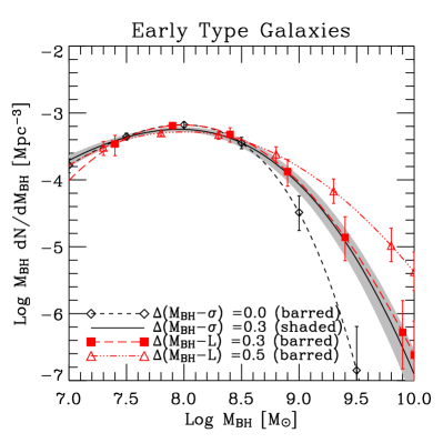
To derive the using the - relation we apply Eq. 3. For the galaxy velocity function we use the parameterized form for early type galaxies by Sheth et al. (2003). For the - relation we use the coefficients obtained by fitting the ‘Group 1’ galaxies of Marconi & Hunt 2003 (i.e. galaxies with ‘secure’ BH mass determinations):
| (8) |
The slope is in agreement with that of Tremaine et al. 2002 () but there is a larger normalization ( i.e. in ). This choice of the coefficients for the - relation is made for consistency since, in the following, we use the coefficients of the - relation determined for the same ’Group 1’ galaxies by Marconi & Hunt (2003). The local ’s derived with the - relation assuming intrinsic dispersions =0 and =0.30 are shown in Fig. 1a. The shaded area and errorbars indicate the 16 and 84% percentiles of 1000 Montecarlo realizations of the local . The realizations were obtained by randomly varying the input parameters assuming that they are normally distributed with 1 uncertainties given by their measurement errors. For the velocity function we have considered only the error on , the number density at , since the other errors are strongly correlated among themselves (Sheth et al. 2003). The 16 and 84% percentiles indicate the uncertainties on the logarithm of the local , whose values from the Montecarlo realizations are normally distributed at a given .
To derive the using the - relation we again apply Eq. 3. The galaxy luminosity function by Bernardi et al. (2003b) is given as a function of the total galaxy light. Since the correlation of is with bulge light, we need to apply a correction in the case of S0 galaxies to transform from total to bulge luminosity. Following Yu & Tremaine (2002), the luminosity function for the bulges of S0 galaxies is directly given by
| (9) |
where is the luminosity function of early type galaxies, is the absolute bulge magnitude, and , are the fractions of E and S0 galaxies with respect to the total galaxy population. The galaxy type fractions and used in this paper are shown in Table 1. The morphological type fractions are from Fukugita, Hogan, & Peebles 1998 (their Sbc fraction has been evenly split between Sab and Scd). The uncertainties are a conservative estimate we made after comparing various determinations of the morphological type fractions available in the literature (see the discussion in Fukugita, Hogan, & Peebles 1998). The for the band are those estimated by Aller & Richstone (2002) by rebinning the Simien & de Vaucouleurs 1986 data in the appropriate bins of galaxy types. The for the band are based on data from Hunt, Pierini, & Giovanardi 2004 and the values for S0 galaxies were taken from the analysis by Marconi & Hunt (2003). The values are little dependent on the photometrical band at least within the considerable scatter, therefore in the following analysis we will always use the band data regardless of the photometric band in which was measured.
| Adopted Luminosity | – | (E+S0) | (All) |
|---|---|---|---|
| or Velocity Function | –host-gal.-prop. | [] | |
| Sheth et al. 2003 | - | ||
| Bernardi et al. 2003 | - | … | |
| Nakamura et al. 2003 | - | ||
| Kochanek et al. 2001 | - | ||
| Marzke et al. 1994 | - | ||
| All L- or V- Func. | … | … | |
Applying the above corrections to the early-type band luminosity function by Bernardi et al. (2003b) and the color transformation we obtain the luminosity function of the bulges of early types in the band. Cole et al. (2001) estimate which, combined with the average value for the early type galaxies (Bernardi et al. 2003b), provides the required color. Fukugita, Shimasaku, & Ichikawa (1995) estimate (E:S0:Sab:Sbc:Scd) and this justifies our conservative choice of the scatter which also allows us to apply the same color correction to all morphological types. For the - relation we use the coefficients obtained by fitting the ’Group 1’ galaxies of Marconi & Hunt (2003) in the band:
| (10) |
where is in units of . The local derived with the - relation assuming intrinsic dispersions =0.30 and =0.5 are plotted in 1a. As before, the 16 and 84% percentiles of 1000 Montecarlo realization of the local indicate uncertainties (shaded area and errorbars).
As clear from Fig. 1a the effect of including the intrinsic dispersion in the - and - correlations is that of softening the high mass decrease of the , thus increasing the total density. But the most important result is that in order to provide the same , the relations - and - must have the same intrinsic dispersion to within 0.1 in log. Yu & Tremaine (2002) found that by using =0 for - and =0.5 for -. This discrepancy can be entirely ascribed to the effect quantified by Eq. 7. Indeed, the densities of the ’s plotted in Fig. 1a are [- with =0, in agreement with Yu & Tremaine (2002)] and [- with =0.5]. Conversely, with =0.30, one obtains (-) and (-) and these two values are in excellent agreement. The densities in massive ’s were evaluated in the range and the same range will be considered throughout the rest of the paper.
One advantage of using the - relation is that the uncertainties on the derived are smaller than in the case of -. This is because with the - relation one does not have to apply any correction for the bulge fraction. On the other hand, measuring stellar velocity dispersions is much more difficult than measuring galaxy luminosities; thus it is clear that the two relations - and - should complement each other.
In summary, the use of the same intrinsic dispersion for the - and - relations provides perfectly consistent ’s with the same mass densities . This is a confirmation of the results by Marconi & Hunt (2003) who showed that, when considering only secure BH measurements, the - - and - relations have similar intrinsic dispersions ( in log). When not taking into account the intrinsic dispersion of the - relation, the local is systematically underestimated at the high mass end, where the disagreement with the of AGN relics has been claimed.
2.3 The Black Hole Mass Function for Early Type Galaxies
Having established that both - and - relations provide consistent ’s we can now evaluate the effects of using luminosity functions from different galaxy surveys and photometric bands in determining the in early type galaxies.
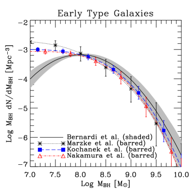
In Fig. 1b we compare the local ’s for early type galaxies obtained from different galaxy luminosity functions, in different photometric bands. We use the luminosity functions by Bernardi et al. (2003b), Marzke et al. (1994), Kochanek et al. (2001), and Nakamura et al. (2003) with details of the derivation specified in the following.
-
•
Bernardi et al. 2003b: this is the same plotted in panel a derived using the - relation.
-
•
Marzke et al. 1994: we use the luminosity functions per morphological type from the CfA survey. The luminosities are in Zwicky magnitudes, , and we apply the color transformations directly measured by Kochanek et al. (2001) computing for all the objects used for the luminosity functions ( is obtained from the 2MASS catalogue): for (E;S0;Sa-Sb;Sc-Sd). The magnitudes used are isophotal magnitudes and the correction to total magnitudes is (Kochanek et al. 2001). Then we use the bulge-total correction and the - relation from Tab. 1.
- •
- •
As in the previous section, uncertainties are estimated with 1000 Montecarlo realizations of the local where, in the case of the galaxy luminosity functions, we use only errors on , the galaxy number density. All the local ’s for early type galaxies are in remarkable agreement within the uncertainties. The discrepancy at the low mass end () between the derived with the Bernardi et al. (2003b) luminosity functions and the others is not significant. It occurs in a region where the luminosity functions of early type galaxies are extrapolated and is due to the different functional forms adopted to fit the data (gaussian for Bernardi et al. (2003b), Schechter functions for the others).
2.4 The Black Hole Mass Function for All Galaxy Types
Here we estimate the local by considering also late morphological types. We use all the luminosity and velocity functions described in the previous section (with the exception of the one by Bernardi et al. (2003b) which is only for early type galaxies). For the velocity function of late type galaxies we take the estimate made by Sheth et al. (2003) and shown in their Fig. 6. When necessary, we apply the bulge-to-total correction with the numbers in Tab. 1 and we then use either the - or the - relation as described in Sec. 2.2.
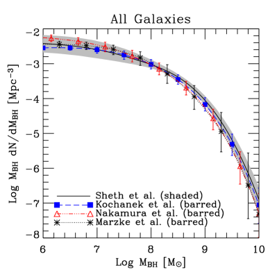
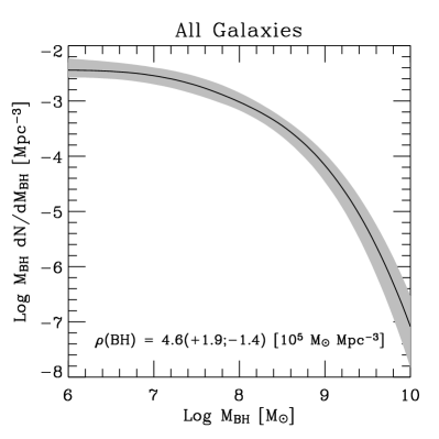
Fig. 2a shows the local for all galaxies while Tab. 2 reports the estimated mass densities both for early type and all galaxies. These densities are computed for . All the ’s and ’s are in agreement within the errors. Finally, in Fig. 2b we present our best estimate of the local obtained by merging all the random realizations of the ’s shown in Fig. 2a and considering the 16, 50 and 84% percentile levels. Our best estimate of the local density in massive BH’s is consequently . Roughly 70% of the total BH density resides in early type galaxies. Our estimate of the density in local ’s is in agreement with Merritt & Ferrarese (2001a) and with Ferrarese (2002) though, in the latter case, the shape of our is very different at the high mass end. Our estimate is a factor larger than those by Yu & Tremaine (2002) and Aller & Richstone (2002) and the reasons for this discrepancy are outlined in Sec. 4.
3 The Mass Function of AGN relics
Once the mass function of local ’s has been determined, the subsequent step is the estimate of the of AGN relics, i.e. ’s in galactic nuclei which were grown exclusively during active phases from small (1-) seeds. We will first describe the continuity equation which will be used to relate the relic , , to the AGN luminosity function , under the assumption that AGN are powered by mass accretion onto massive ’s. The physical quantity directly related to the mass accretion onto the BH is the total intrinsic AGN luminosity . Since AGN luminosity functions are determined in limited energy bands, we will provide suitable bolometric corrections. We will then briefly describe the adopted AGN luminosity functions obtained with our bolometric corrections. Finally we will present our estimates of the relic BHMF’s derived from different AGN luminosity functions.
3.1 The Continuity Equation
The Black Hole Mass Function of AGN relics, , can be estimated from the continuity equation (Cavaliere, Morrison, & Wood 1971; Small & Blandford 1992) with which, under simple assumptions, it is possible to relate to the AGN luminosity function. If is the comoving number density of ’s with mass in the range and at cosmic time , the continuity equation can be written as:
| (11) |
where is the ”average” accretion rate on the BH of mass . We adopt the working assumption that AGN’s are powered by accretion onto ’s, and that the growth takes place during phases in which the AGN is accreting at a fraction of the Eddington limit () converting mass into energy with an efficiency . We can thus simply relate the AGN Luminosity Function [ is the comoving number density of AGNs in the range at cosmic time ] to the mass function:
| (12) |
where is the fraction of ’s with mass which are active at time , i.e. the duty cycle. If a is accreting at a fraction of the Eddington rate, its emitted luminosity is
| (13) |
where is the Eddington time, is the accretion efficiency and is the matter falling onto the black hole. The growth rate of the , , is thus given by , since a fraction of the accreted mass is converted into energy and thus escapes the BH. Since , combining Eqs. 12 and 13 we can write:
| (14) |
which can be placed in Eq. 11 where the only unknown function is . If and are constant we can then write
| (15) |
which can be easily integrated given the AGN luminosity function and the initial conditions.
For initial condition, we assume that, at the starting redshift , . This can be interpreted either by saying that at all Black Holes are active or that we are following the evolution only of those ’s which were active at . Thus
| (16) |
We will show that the final results are little sensitive to the choice of the initial conditions, provided that , since most of the growth takes place at lower redshifts.
Eq. 15, which represents the continuity equation in the case of constant and , can be trivially integrated on to derive the relation used by various authors (Padovani, Burg, & Edelson 1990; Chokshi & Turner 1992; Yu & Tremaine 2002; Ferrarese 2002):
| (17) |
note the factor which is needed to account for the part of the accreting matter which is radiated away during the accretion process. is the total comoving energy density from AGN’s (not to be confused with the total observed energy density) and is given by
| (18) |
is used if the AGN luminosity function is defined per logarithmic luminosity bin, otherwise it should be .
The right-hand element of the continuity equation, which contains the source function, is null, meaning that we neglect any process which, at time , might ‘create’ or ‘destroy’ a with mass . Indeed, in the merging process of two ’s, , ’s with and are destroyed while a BH with is created. We decided to neglect merging of ’s because, at present, the merging rate, , is very uncertain and dependent on the assumptions of the model with which it is computed. Moreover, the aim of this paper is to assess if local ’s are indeed relics of AGN activity and by neglecting merging we can assess the importance of mass accretion during AGN phases. Yu & Tremaine (2002) have used an integral version of the continuity equation in order to take into account merging but their approach does not allow a direct comparison of the local and relic ’s. Furthermore, the discrepancy they find between local ’s and AGN relics becomes worse if merging is important. Granato et al. (2004) in their physical model of coevolution of and host galaxy find that the growth of the is due to mass accretion. Similarly, Haiman, Ciotti, & Ostriker (2003) find that merging of BH’s is important only at high redshifts while, at lower , BH growth is dominated by mass accretion. These reasons support our choice of neglecting the merging process. Indeed merging of ’s might well be very important in shaping the at high redshifts () but, as we will see, the relic at is very little dependent on its shape and normalization at . Moreover, if the relic at is changed significantly by merging then its remarkable agreement with the local in the merging-free case would be a mysterious coincidence (see Sec. 4).
3.2 The Bolometric Corrections

The mass accretion rate is given by the AGN luminosity which, in turn, can be estimated from the luminosity in a given band , , by applying a suitable bolometric correction . At the beginning of Sec. 3 we have referred to as the total intrinsic AGN luminosity, and before presenting the adopted bolometric corrections it is necessary to define the meaning of intrinsic.
The integral of the observed spectral energy distribution (SED) of an AGN provides the total observed luminosity, , thus the quasar bolometric corrections by Elvis et al. (1994) provide because they are based on the average observed SED. However, does not give an accurate estimate of the BH mass accretion rate because it often includes reprocessed radiation (i.e. radiation absorbed along other lines of sight and re-emitted isotropically). The accretion rate is better related to the total luminosity directly produced by the accretion process, which we call the total intrinsic luminosity . In AGN’s, is given by sum of the Optical-UV and X-ray luminosities radiated by the accretion disk and hot corona, respectively. Conversely, it is well known that the IR radiation is reprocessed from the UV (e.g. Antonucci 1993). Thus, in order to estimate one has to remove the IR bump from the observed SED’s of unobscured AGN’s. In radio loud AGN’s there might be an important contribution from synchrotron radiation to the IR. However this will not affect our average bolometric corrections since the number of radio loud AGN’s is small, of the whole AGN population.
In previous works, several authors have used the bolometric corrections by Elvis et al. (1994) but, as explained above, these provide the observed and not the intrinsic AGN luminosity. Removing the IR bump from the Elvis et al. 1994 spectral templates, the 1-X-ray range includes of the total energy; thus one obtains, for instance, instead of the commonly used . However, the Elvis et al. 1994 quasar templates, obtained from an X-ray selected sample of quasars, are X-ray “bright” (see the discussion in Elvis, Risaliti, & Zamorani 2002) and thus underestimate the bolometric corrections in the X-ray energy bands. Moreover the dependence on luminosity of the bolometric corrections cannot be obtained. For these reasons we will derive new estimates of the bolometric corrections as described in the following.
First, we construct a template spectrum. In the optical-UV region our template consists of a broken power-law with () in the range Å and in the range 1200-500Å (e.g. Telfer et al. 2002; Vanden Berk et al. 2001). At our big blue bump is truncated assuming as in the Rayleigh-Jeans tail of a blackbody. The X-ray spectrum beyond 1 keV consists of a single power law plus a reflection component. The powerlaw has the typical photon index (e.g. George et al. 1998; Perola et al. 2002) and an exponential cutoff at . Following Ueda et al. (2003), the reflection component is generated with the pexrav model (Magdziarz & Zdziarski 1995) in the XSPEC package with a reflection solid angle of , inclination angle of and solar abundances. We then rescale the X-ray spectrum to a given (Zamorani et al. 1981) which is defined as
| (19) |
and we finally connect with a simple powerlaw the point at 500Å with that at 1. To account for the dependence of on luminosity, we use the relation by Vignali, Brandt, & Schneider (2003):
| (20) |
Finally, we assume that the template spectra, hence the bolometric corrections, are independent of redshift.
The template spectrum for a AGN is plotted in Fig. 3a and is compared with the radio quiet and radio loud quasar median spectra by Elvis et al. (1994). Our template is in very good agreement in the optical-UV part but is obviously missing the IR bump, which is due to reprocessed UV radiation and thus not considered here. Our template is fainter in X-rays but this is expected since, as already discussed, the quasar sample by Elvis et al. (1994) is X-ray bright.
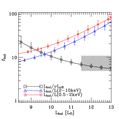
In Fig. 3b we plot the bolometric corrections , and derived from the above templates. The errorbars lines represent the 16 and 84% percentiles from 1000 Montecarlo realization of the spectral templates where we have assumed the following uncertainties for the input parameters: for the spectral slopes (; Telfer et al. 2002; Vanden Berk et al. 2001) in the 1-500Å range and for the , constant at all luminosities. The latter is a conservative assumption (see, e.g., Yuan et al. 1998) but is made to account for possible, but unaccounted for, systematic errors. As in the case of the local , the 16 and 84% percentiles correspond to uncertainties on the logarithm of the bolometric corrections. The 50% percentiles can be fit with a 3rd degree polynomial to obtain the following convenient relations:
| (21) | |||||
where and is the bolometric luminosity in units of . Hence, the bolometric corrections have log-normal distributions with average values given by the above equations and scatters (at fixed ) which can be derived from Fig. 3b. Scatters are given by for the B band and for the X-rays, taken independent of for simplicity. It is worth noting that the B band bolometric correction is in agreement with that by Elvis et al. (1994) whose average value and scatter are shown by the hatched area in Fig. 3b. The scatter of the Elvis et al. (1994) bolometric correction is the standard deviation of their quasar sample while ours are uncertainties on the average values. The average in the range is 1.43, the same value estimated by Elvis, Risaliti, & Zamorani (2002) after correcting for the biases due to X-ray or optical selection of the parent quasar samples.
3.3 The Luminosity Function of Active Galactic Nuclei
In order to ensure a consistent treatment, the AGN luminosity function used in the continuity equation must describe the evolution of the entire AGN population. The luminosity is the total luminosity radiated from the accreting mass and is estimated with the bolometric corrections described in the previous section.
The AGN luminosity functions available in the literature do not describe the entire AGN population because they are the result of surveys performed in ”narrow” spectral bands, with given flux limits and selection criteria. For example, the luminosity function of Boyle et al. (2000) includes only quasars selected for their blue color but it is now known there is a population of ”red” quasars which is missed. The luminosity function of soft X-ray (0.5-2 keV) selected AGNs of Miyaji, Hasinger, & Schmidt (2000) misses most of the sources with significant X-ray absorption (); it includes mostly broad lined AGNs ( of the total) but it is known that, at least locally, there is a dominant population of obscured AGN’s (e.g. Maiolino & Rieke 1995). Current hard X-rays surveys (2-10 keV) are less sensitive to obscuration than optical and soft X-ray ones, thus the very recent luminosity function by Ueda et al. (2003) probes by far the largest fraction of the whole AGN population. However it is restricted only to Compton-thin AGNs (), while it is known that, at least locally, there is a significant fraction of Compton-thick objects (e.g. Risaliti, Maiolino, & Salvati 1999). In summary, when using the luminosity functions available in the literature, one should know that they describe part of the AGN population, and thus account only for a fraction of the local .
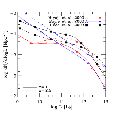
In this paper, we consider the AGN luminosity functions by Boyle et al. 2000 (band ), Miyaji, Hasinger, & Schmidt 2000 (0.5-2 keV) and Ueda et al. 2003 (2-10 keV). Thus, the AGN luminosity function which will be used in the continuity equation is given by
| (22) |
where is either the , the 0.5-2 keV or the 2-10 keV band and .
The AGN luminosity functions obtained with the bolometric corrections described in the previous section are compared in Fig. 4a at selected redshifts. The luminosity functions by Boyle et al. (2000) and Miyaji, Hasinger, & Schmidt (2000) are in rough agreement at the high end, meaning that they may be sampling the same quasar population. Indeed most of the objects in the Miyaji, Hasinger, & Schmidt (2000) sample are broad-lined AGN which, at high , become the quasars observed by Boyle et al. (2000). The disagreement at low luminosities is because the Boyle et al. 2000 luminosity function is extrapolated for i.e. for . In contrast the luminosity function by Ueda et al. (2003) samples a larger fraction of the AGN population at all luminosities.
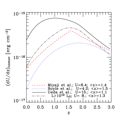
In Fig. 4b we compare the differential comoving energy densities computed in the luminosity ranges ( and bands) and ( band). For the Ueda et al. (2003) luminosity function we also plot the differential comoving energy density for objects with . High luminosity objects provide of the total energy density in the Ueda et al. (2003) luminosity function and their emission has a redshift distribution similar to that of the AGN’s by Miyaji, Hasinger, & Schmidt (2000) and Boyle et al. (2000). Clearly, lower luminosity objects contribute significantly at and this is an important result of the recent Chandra and XMM surveys (e.g. Hasinger 2003; Fiore et al. 2003; Ueda et al. 2003). The total comoving energy densities in the redshift range (i.e. the integrals of the quantities plotted in the figure) are 4.2, 6.4 and 1.5-3, for Boyle et al. 2000, Miyaji, Hasinger, & Schmidt 2000, and Ueda et al. 2003, respectively. The high objects in the Ueda et al. (2003) luminosity function provide 8-3, i.e. of the total energy density.
By applying Eq. 17, the mass densities in BH’s can be written as
| (23) |
where is 0.6 (from the Boyle et al. 2000 AGN LF), 0.9 (Miyaji, Hasinger, & Schmidt 2000), 2.2 (Ueda et al. 2003) and 1.2 (Ueda et al. 2003, high objects). The value derived from the Ueda et al. (2003) luminosity function () is already in marginal agreement with , i.e. the estimate of the local BH density given in Sec. 2.4.
3.4 The Relics of Active Galactic Nuclei
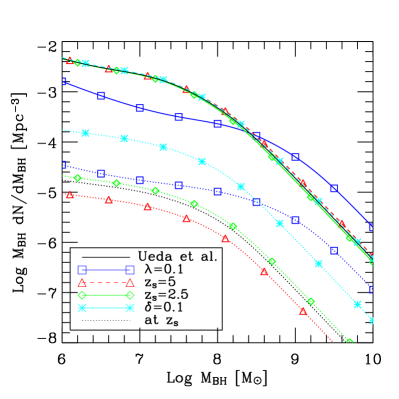
Given the AGN luminosity functions (Boyle et al. 2000; Miyaji, Hasinger, & Schmidt 2000; Ueda et al. 2003) we can integrate the continuity equation assuming that (AGN’s emitting at the Eddington luminosity), and =3. Though we know that the above luminosity functions do not describe the whole AGN population, initially we do not apply any correction for the objects which have been missed.
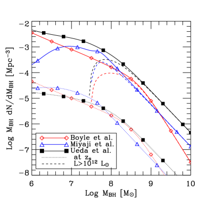
The relic BH mass functions are shown in Fig. 5a. As expected, the AGN’s traced by the Ueda et al. (2003) luminosity function leave more relics than those traced by the luminosity functions of Boyle et al. (2000) and Miyaji, Hasinger, & Schmidt (2000). It is also notable that the relic ’s at (solid lines) are order of magnitude larger than those at (dotted lines) meaning that most of the BH growth took place for . The dashed lines represent the relic obtained by considering only AGN’s with . [In practice this was obtained by multiplying the AGN luminosity functions by .] The comparison between the dashed and solid lines indicate that today high mass BH’s () grew during quasar phases ().
The ’s in Fig. 5a were estimated assuming and . It can be seen from Eq. 15 that the efficiency is a simple scaling factor and an increase in will decrease the level of the relic . However a variation of the Eddington fraction will not have a simple scaling effect but it will produce a combination of scaling and translation along the axis since also enters the relation. In Fig. 5b the same relic derived using Ueda et al. 2003 (thick line with no symbols) is compared with the obtained assuming (line with empty squares). As previously, solid and dotted lines indicate the at and at respectively. Decreasing has the net effect of increasing the number of ’s at high masses () while decreasing that at lower masses. In the same figure, we also show the ’s obtained by assuming that the starting redshift of integration is (line with empty triangles) and (line with empty diamonds) and that the fraction of active BH’s at is instead of 1 (line with stars). The relic at is almost independent of the initial conditions. Changing the starting assumption (, or ) does not have any appreciable effect provided that . This is a consequence of the fact that the main BH growth takes place at when there is more time available (% of the age of the universe). At larger redshifts there is too little time for the BH growth.
In summary, relic BH’s grew mainly at low redshifts () and high mass BH’s were produced during quasar activity. The initial conditions for the continuity equation influence little the relic at .
4 Local BH’s and AGN Relics
In this section we compare the local and relic ’s. At first we will consider the relic ’s derived in the previous section, without trying to account for the AGN population missing in the adopted luminosity functions. After showing that, as expected, the Ueda et al. (2003) luminosity function encompasses the largest fraction of the AGN population, thus providing a better match to the local , we will focus on it and try to account for the missing AGN’s in a way which also satisfies the constraints imposed by the X-ray background.
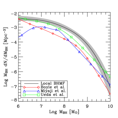
In Fig. 6a we compare the local derived in Sec. 2.4 (Fig. 2b) with the relic ’s obtained adopting the Boyle et al. (2000), Miyaji, Hasinger, & Schmidt (2000), and Ueda et al. (2003) AGN luminosity functions (, ) without any correction for the missing AGN population. As shown in the previous section these relic ’s are insensitive to the adopted initial conditions thus the parameters they depend on are only and .
The first result which can be evinced from the figure is that there is no discrepancy at high masses. All the relic ’s are slightly smaller than the local . As explained previously, this is not significant because all the adopted luminosity functions are missing part of the AGN population. Conversely Yu & Tremaine (2002) and Ferrarese (2002) using the Boyle et al. (2000) luminosity function found a significant discrepancy because their relic at high masses is larger than the local one. The reasons for the solution of this discrepancy are the following.
-
•
We have taken into account the intrinsic dispersion of the - and - correlations thus softening the high mass decrease of the local .
-
•
We have adopted zero points in the - and - correlations which are a factor ( in log) larger than those used by Yu & Tremaine (2002). These zero points (and slopes) were derived from the analysis of Marconi & Hunt (2003) and their larger value is a consequence of the rejection of galaxies with unreliable masses.
-
•
We have adopted bolometric corrections which, on average, are of those adopted by previous authors. This is because we have not taken into account the IR emission in the estimate of the bolometric luminosity. The IR bump is produced by reprocessed UV radiation and thus its use in the determination of would result in overestimated accretion rates.
We now focus on the Ueda et al. (2003) AGN luminosity function since we have established that, as expected, it is the one which provides the most complete description of the AGN population. The aim is to assess whether the relic can account for the whole local , i.e. if local ’s can be entirely explained as being AGN relics.
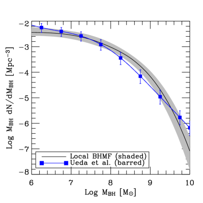
The Ueda et al. (2003) luminosity function only describes the population of Compton-thin AGN’s, i.e. objects with absorbing column densities [-2]. To estimate the correction for the missing Compton-thick sources, we follow Ueda et al. (2003) and assume that there are as many AGN’s in the 24-25 bin of as in the 23-24 one, as indicated by the distribution of Risaliti, Maiolino, & Salvati 1999. Thus, with the distribution estimated by Ueda et al. (2003), the luminosity function has to be multiplied by 1.3 in order to account for the Compton-thick AGN’s. In reality, the correcting factor is luminosity dependent but, since it is limited to the range, we chose an average value for simplicity. With this contribution from Compton-thick sources, Ueda et al. (2003) are able to provide a reasonable fit of the X-ray background spectrum. (We will return to this issue in the following section.) While AGN’s at are not important contributors of the X-ray background, they do contribute to the relic . Thus, we assume that for there are as many AGN’s as in the 23-24 or 24-25 bins. This assumption is also justified by the Risaliti, Maiolino, & Salvati (1999) distribution. The correcting factor becomes then 1.6. Therefore, to compensate for the missing obscured AGN’s we apply a correcting factor of 1.6 independently of luminosity. In Fig. 6b the corrected Ueda et al. (2003) luminosity function is used to determine the relic . We also show the uncertainties (16 and 84% percentiles, i.e. errors on the log of the relic as previously) estimated with the usual 1000 Montecarlo realizations of the relic . These were obtained by varying the number density of the luminosity function ( error on the number density to avoid correlated errors on the other parameters), the hard X-ray bolometric correction ( error on ), and the factor used to correct for the missing Compton-thick AGN’s ( error).
The relic and local agree well within the uncertainties. Thus, adopting the best possible description of the whole AGN population, the mass function of relic ’s is in excellent agreement with the mass function of local ’s. Local ’s are thus AGN relics and were mainly grown during active phases in the life of the host galaxy. This agreement has been obtained with and indicating that (i) efficiencies higher than commonly adopted for AGN’s are not required, and (ii) the main growth of BH’s occurs in phases during which the AGN is emitting close to the Eddington limit. In Section 6 we will explore the locus in the plane which is permitted by the comparison from the local and relic ’s. As discussed in Section 3.1 we have neglected merging in our estimate of the relic . However, the good agreement between the local and relic ’s suggests that the merging process does not significantly affect the build-up of the , at least in the redshift range.
5 Constraints from the X-ray Background
From the X-ray background (XRB) light it is possible to estimate the expected mass density of relic BH’s (Salucci et al. 1999; Fabian & Iwasawa 1999; Elvis, Risaliti, & Zamorani 2002) which can then be compared with the mass density of local BH’s. From this comparison, Elvis, Risaliti, & Zamorani (2002) inferred that massive BH’s must be rapidly rotating for the high efficiency needed () to match the XRB and local BH mass densities. We will show that, due to the redshift distribution inferred from the new X-ray surveys, the match between the XRB and local BH mass densities can be obtained without requiring large efficiencies (; see also Fabian 2003; Comastri 2003).
The XRB provides another type of constraint. It has been shown (Setti & Woltjer 1989; Madau, Ghisellini, & Fabian 1994; Comastri et al. 1995; Gilli, Risaliti, & Salvati 1999) that the XRB spectrum can be reproduced by summing the spectra of the whole AGN population after suitable corrections to take into account the absorption along the line of sight. The AGN population and its redshift distribution is derived from AGN luminosity functions but, in order to fit the XRB spectrum, one has to include a correction for the missing (obscured) AGN’s. This correction is the same one which must be adopted here to determine the relic from the whole AGN population. Thus, the ratio between AGN’s included and missed in the adopted luminosity functions is a parameter which determines both the relic and the XRB spectrum (and the X-ray source counts). When rescaling the AGN luminosity function with the factor to match the local , one should also verify that it is also possible to match the XRB spectrum and source counts at the same time. In practice, one can use the value required by the XRB synthesis models in order to fit the XRB spectrum and source counts. It is beyond the scope of this paper to produce a model synthesis of the XRB but we will show that with values found in the literature we can match the local and relic , and also satisfy the constraints imposed by the X-ray background.
The local density in massive BH’s expected from the observed X-ray background (XRB) light can be estimated with the relation
| (24) |
where is the total observed (as opposed to comoving) AGN energy density and is the average source redshift. The factor is needed to take into account the fact that not all the accreting mass falls into the . can be estimated from the observed X-ray background light as
| (25) |
where is the total observed surface brightness of the X-ray background (i.e. the integral of the XRB spectrum), is the correction to take into account source obscuration in the X-rays (i.e. would be the total XRB surface brightness if AGN’s were not obscured) and is the X-ray bolometric correction (see for more details Fabian & Iwasawa 1999; Salucci et al. 1999; Elvis, Risaliti, & Zamorani 2002). Elvis, Risaliti, & Zamorani (2002) estimate .
We first verify that the above formula is consistent with the scheme followed in this paper, and then establish how must be computed. The observed background surface brightness at energy is
| (26) | |||||
where is the luminosity distance, is the comoving volume, is the source luminosity in the energy band and is the luminosity function in the same band. is the source spectrum at energy normalized to have unit luminosity in the band . Integrating on to find the total surface brightness in band one finds
| (27) |
Applying the bolometric correction ( with = ), the obscuration correction () and comparing with Eq. 18, one finds that
| (28) |
where and is the total comoving (as opposed to observed) energy density. The average redshift is then
| (29) |
Using the luminosity function by Ueda et al. (2003) one finds , lower than the value assumed by previous authors. For comparison, the high luminosity objects () in the Ueda et al. (2003) luminosity function have while the Miyaji, Hasinger, & Schmidt (2000) and Boyle et al. (2000) have and , respectively. With the estimate by Elvis, Risaliti, & Zamorani (2002) we get
| (30) |
which is perfectly consistent with the estimate from the local BHMF without requiring efficiencies larger than the ‘canonical’ value =0.1. This agreement has also been remarked by Fabian 2003 and Comastri 2003. The critical point is clearly the value of , the average redshift of X-ray sources emitting the XRB, which has been significantly reduced by Chandra and XMM surveys (e.g. Hasinger 2003; Fiore et al. 2003; Steffen et al. 2003; Ueda et al. 2003). The minimum value of , allowed for a consistency between the two estimates of , is just slightly larger than the non-rotating BH case. Conversely, the maximum allowed efficiency is , substantially below the maximally rotating Kerr BH case (see Sec. 6). It is intriguing to find that efficiencies smaller than those expected from non-rotating BH’s or larger that those expected from maximally rotating Kerr BH’s are excluded.
We have thus verified that the expected density of BH remnants inferred from the XRB is consistent with the local one without requiring efficiencies larger than the canonically adopted value . We now verify if, with the obscured/unobscured ratios adopted in XRB synthesis models, it is possible to reproduce also the local . For the scope of this paper it suffices to notice that the Ueda et al. (2003) luminosity function, with the correction for the missing Compton-thick AGN’s that we also adopt, is used by the same authors to successfully reproduce the XRB spectrum and source counts. Thus the agreement of the local and the relic in Fig. 6b is obtained by also meeting the constraints from the XRB which, in practice, provide an estimate of the number of AGN’s missed by the luminosity function. The same comparison could also be done using the Miyaji, Hasinger, & Schmidt (2000) luminosity function combined with the background model of Gilli, Salvati, & Hasinger (2001). However, though that model is successful in reproducing the XRB spectrum and source counts, recent Chandra and XMM surveys have shown that the model redshift distribution is not correct (e.g. Hasinger 2003).
In summary, our analysis shows that it is possible to meet the XRB constraints both in terms of and of the local .
6 Accretion Efficiency and Eddington Ratio
The relic derived from the Ueda et al. (2003) AGN luminosity function, corrected for the Compton-thick AGN’s, provides a good match to the local and also satisfies the XRB constraints. The match is obtained for and . Here we investigate the locus in the plane where an acceptable match of the local and relic ’s can be found, i.e. we determine the acceptable and values.
To quantify the comparison between the local and relic ’s we recall that all the realizations of the ’s have a log-normal distribution at given and we consider the following expression:
| (31) |
where and are the local and relic ’s with their uncertainties, and . The integration is performed in the range. is the average square deviation between the logarithms of the two ’s measured in units of the total standard deviation. If, for instance, , then , i.e. the two functions differ, on average, by times the total standard deviation.
The and values that corresponds to the minimum () are marked by the filled square and are and . To have an acceptable match between the local and relic we require that and this constraint identifies the region limited by the solid line in Fig. 7. For comparison, the dashed line limits the region where , which corresponds to the average square deviation in the ”canonical” case, and , which is marked by the cross. The allowed efficiencies include the non-rotating Schwarzschild (, Schwarzschild 1916; Shapiro & Teukolsky 1983) and are well below the maximally rotating Kerr (, Kerr 1963; Shapiro & Teukolsky 1983). The best agreement between the local and relic ’s is obtained for efficiencies larger than that of the non-rotating case suggesting that, on average, ’s should be rotating. Hughes & Blandford (2003) found that ’s are typically spun down by mergers and this would limit the importance of mergers in the growth of ’s, in agreement with our assumption in the continuity equation.
The allowed Eddington ratios, , are in the range indicating that growth takes place during luminous accretion phases close to the Eddington limit. McLure & Dunlop (2003), using a large sample of SDSS quasars, have recently estimated that the average varies from 0.1 at to 0.4 at . Accounting for the different bolometric corrections (they used , times larger than the value adopted by us), varies from 0.15 at to 0.6 at . These values are in excellent agreement with the constraints posed on in Fig. 7.
The results in Fig. 7 do not imply that accreting BH’s cannot have and values outside the region of the best match between the local and relic ’s. Indeed, those limits are only for average efficiencies and Eddington ratios during phases in which Black Holes are significantly grown.

We conclude by noting that represents only the radiative efficiency. If there is significant release of mechanical energy, the true efficiency might be higher. For instance, in M87 the kinetic energy carried away by the jet is much larger than the radiated one (Owen, Eilek, & Kassim 2000) and, in general, the jets of radio loud AGN’s can carry away up to half of the total power in kinetic energy (Rawlings & Saunders 1991; Celotti, Padovani, & Ghisellini 1997; Tavecchio et al. 2000). The release of mechanical and radiative energy is important for the feedback on the galaxy which is thought to be one of the causes behind the - and - correlations (e.g. Silk & Rees 1998; Blandford 1999; Begelman 2003; Granato et al. 2004). Taking into account mechanical energy, the expression should be transformed to , where and are the radiative and mechanical efficiencies. Then, similarly, to what has been done in section, one could place constraints on both and but this is beyond the scope of this paper.

7 Growth and Accretion History of Massive Black Holes
Having established that the obscuration corrected AGN luminosity function by Ueda et al. (2003) with and provides a relic which is fully consistent with the local and the X-ray background, we can analyze the growth history of massive ’s and, in the next section, the average lifetime of their active phases.
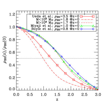
The redshift dependence of the total density in massive BH’s is given by (Eqs. 17 and 18)
| (32) |
and is plotted in Fig. 8a. The relics of the AGN’s traced with the luminosity functions by Boyle et al. (2000) and Miyaji, Hasinger, & Schmidt (2000) reach 50% of the mass density around , while the AGN’s traced by the Ueda et al. (2003) luminosity function do so at . This is a consequence of the larger number of low luminosity AGN’s which are present at (see also Fig. 4b). Indeed, when separating the contributions from low () and high mass ’s which contribute 50% each of the density, it is clear that low mass ’s grow later than high mass ’s. These, like in the case of the AGN’s traced by Boyle et al. (2000) and Miyaji, Hasinger, & Schmidt (2000), reach 50% of their final mass at .
This issue can be further investigated by computing the average growth history of a with given starting, or final, mass. The growth history of a with given starting mass at can be estimated as follows. The average accretion rate at (or ) is given from Eq. 15 as:
| (33) |
thus one can solve the following differential equation to obtain the ’average’ growth history of ’s:
| (34) |
In Fig. 8b we plot the average growth history of ’s with different masses at . A supermassive BH like that of M87 or Cygnus A (; Marconi et al. 1997; Tadhunter et al. 2003) was already quite massive () at while a smaller BH like that of Centaurus A (Marconi et al. 2001) was less massive, around . A supermassive BH with at should now be over . Indeed, the existence of very massive ’s at high redshifts is suggested by the detection of very luminous quasars and, in particular, those detected at by the SDSS survey (e.g. Fan 2003). For instance, for the farther quasar known () is estimated as (Willott, McLure, & Jarvis 2003), and one would expect its local counterpart to be more massive than . However, these quasars have not been detected yet and it is not clear if this is because these hypermassive ’s are very rare or they simply do not exist. In the latter case there should be a physical reason which prevents a from growing beyond , possibly the feedback on the host galaxy mentioned in the previous sections (see also Netzer 2003).
From Fig. 8b we can also infer a confirmation of what already found in Fig. 8a, namely that more massive ’s grow earlier. The symbols in the figure, filled squares, empty squares, and stars, mark the points when a reaches 90%, 50%, and 5% of its mass, respectively. It is clear that for all ’s gain more than 95% of their final mass but ’s which are now more massive than had already gained 50% of their mass at . Conversely, ’s which have now masses around grew very recently, at . Again, this is a consequence of the luminosity function by Ueda et al. (2003) in which the distribution of lower luminosity AGN’s peaks at . Thus, the luminosity function of Ueda et al. (2003) points toward an anti-hierarchical growth of ’s in the sense that the largest ’s were formed earlier.
If the correlations between and host galaxy properties were valid at higher redshifts (as is suggested by the results of Shields et al. 2003) this would immediately imply that also the most massive galaxies should form earlier, in contrast with the predictions of current semi-analytic models of galaxy formation (see the introduction of Granato et al. (2004) for more details and references). The detection of high mass galaxies in sub-mm surveys is indeed more consistent with the ‘monolithic’ scenario in which massive ellipticals form at relatively high redshifts (e.g. Genzel et al. 2003; Granato et al. 2004 and references therein).
The BH accretion history (i.e. the total accretion rate at given per unit comoving volume) can be estimated using Eq. 14 as
| (35) |
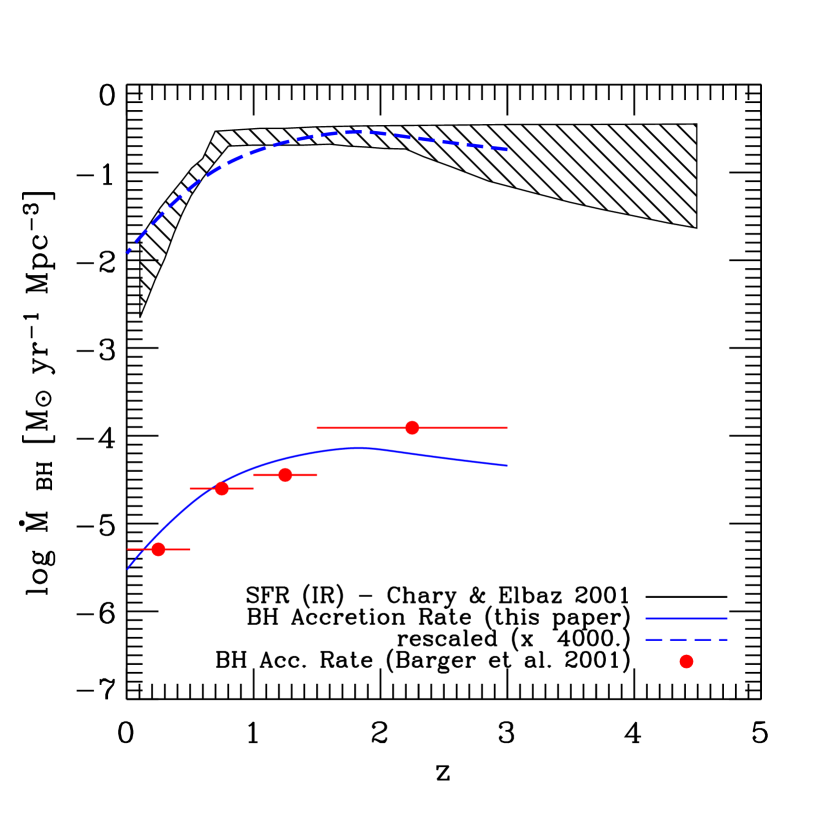
In Fig. 9 we plot the cosmic accretion history of ’s (computed using the Ueda et al. (2003) luminosity function, and ) and we compare it with the estimate by Barger et al. (2001) and with the cosmic star formation rate by Chary & Elbaz (2001).
Our estimate of the cosmic accretion rate onto ’s agrees well with that by Barger et al. (2001), likely because most of the high redshift AGN’s used by Ueda et al. (2003) come from the Barger et al. (2001) sample. Differently from us, Barger et al. (2001) estimate the bolometric AGN luminosities by integrating the observed spectral energy distributions. Thus the agreement with our analysis should be viewed as a consistency check on the bolometric corrections and on the corrections for obscured AGN’s that we applied.
The cosmic accretion history has a similar redshift dependence as the cosmic star formation rate, which we report here in the form estimated by Chary & Elbaz (2001). To aid the eye, the dashed line represents the estimate of the cosmic accretion history rescaled by 4000. The comparison suggests that indeed the two rates have a similar redshift dependence and justifies the assumption that the accretion onto a BH is proportional to the star formation rate, at least at a cosmic level. This fundamental assumption is made in several models of coeval evolution of and galaxy and, together, with the feedback from the AGN explains the observed correlations - and - (e.g. Granato et al. 2004; Haiman, Ciotti, & Ostriker 2003).
8 The lifetime of active BH’s
We now estimate the average lifetime of active BH’s with the formalism used in this paper and the corrected AGN luminosity function by Ueda et al. (2003).
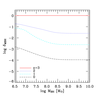
In Fig. 10a we plot the duty cycle at selected redshifts derived from Eq. 12 and computed using the Ueda et al. (2003) luminosity function, and . From Sec. 3.1, the duty cycle is the fraction of ’s with mass active at time or redshift . According to the definitions used in this paper, we consider a active if it is emitting at the adopted fraction of the Eddington luminosity. Hence, objects which are usually classified as ‘active’ but which are emitting well below their Eddington limit (e.g. M87 or Centaurus A), should not be counted among the active BH’s whose fraction is given by the duty cycle. ’s more massive than are very rarely active in the local universe (only 1 out of 10000) while they become more numerous at higher redshifts (by a factor at ). Conversely, lower mass ’s are usually a factor 10 more numerous. A unit duty cycle at is the initial condition assumed for the solution of the continuity equation (see Secs. 3.1 and 3.4). The values of the duty cycle we obtain at are consistent with the average values of estimated by Haiman, Ciotti, & Ostriker (2003).
The average duration of the accretion process, i.e. the mean lifetime of an AGN which has left a relic of mass , is estimated by first solving Eq. 34 to obtain , the growth history of a BH with mass at . Then the ’active’ time is simply given by
| (36) |
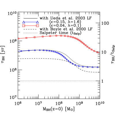
In Fig. 10b we plot the average mean lifetime of AGN’s (solid line) as a function of the relic BH mass at computed using the Ueda et al. (2003) AGN luminosity function and , . The average lifetime of AGN’s which leave a relic BH mass of is of the order of 1.5, while for smaller relic masses () longer active phases are needed (). Considering two limiting cases from Fig. 7, , and , the average lifetimes can increase up to . We remark that these numbers are the average lifetimes for with =3.
The derived lifetimes are consistent with the main result from this paper that most of the masses are assembled via mass accretion. Indeed, if a grows by accreting matter with efficiency and emitting at a fraction of its Eddington luminosity, its e-folding time is given by , the Salpeter time (Salpeter 1964),
| (37) |
Thus, the initial mass has been e-folded times from for and more than 10 times for . The apparently long lifetimes are thus the natural consequence of the fact that to grow a from small () or intermediate mass seeds (, e.g. Schneider et al. 2002) several e-folding times must pass easily implying . For instance, to grow a from to with and , one would need i.e. (see also Haiman & Loeb 2001). Indeed, in the model by Granato et al. (2004) of coeval evolution of and galaxy, the time needed to grow most of the mass is (note however that they use , with which the Salpeter time is roughly halved with respect to our paper).
The reason why the growth of smaller ’s () requires longer time is not obvious but can be understood from Fig. 8b. Consider, for instance, ’s with masses and at . Their average growth history is traced by the lower and upper tracks in the figure. The larger has at and has to e-fold its mass by 3 times. Conversely, the smaller has at and has to e-fold its mass by at least ten times. The masses of large ’s () increase by smaller factors from their values, compared to the masses of smaller ’s. Thus they require shorter active phases.
In general, literature estimates of AGN lifetimes range from to and are still much uncertain (see the review by Martini 2003). Models where ’s grow by a combination of gas accretion traced by short-lived () QSO activity and merging in hierarchically merging galaxies are consistent with a wide range of observations in the redshift range (Haehnelt 2003). However it is not surprising to find a discrepancy with our analysis since we do not consider merging and the growth history that we find is anti-hierarchical. Our estimates agree better with models in which ’s are mainly grown by gas accretion (e.g. Haiman, Ciotti, & Ostriker 2003; Granato et al. 2004).
With an estimate of AGN lifetime based on demographics similar to the one presented here Yu & Tremaine (2002) find for the luminous quasars using the AGN luminosity function by Boyle et al. (2000). The main reason our estimate is larger is that the Ueda et al. (2003) luminosity function has a larger number density of objects, which results in longer lifetimes. Indeed, the quasar lifetimes computed using the luminosity function by Boyle et al. (2000) are (dashed line in Fig. 10b), in agreement with Yu & Tremaine (2002).
Comparing to observational-based estimates, the lifetimes from this paper are in agreement with the results from the length of radio jets (see Martini 2003 for more details). More recently, Miller et al. (2003) found from SDSS data that a very high fraction of galaxies host an AGN () suggesting lifetimes longer than previously thought (i.e. ). Finally, our estimate is in agreement with the upper limit of set by the timescale over which the quasar luminosity density rises and falls (see, e.g., Osmer 2003).
In summary, we estimate that local high mass BH’s () have been active, on average, . On the contrary, the assembly of lower mass ’s has required active phases lasting at least three times that much (). These average lifetimes can be as large as if one considers the smaller efficiency and fraction of Eddington luminosity which are still compatible with local ’s (, ).
9 Conclusions
We have quantified the importance of mass accretion during AGN phases in the growth of supermassive black holes () by comparing the mass function of black holes in the local universe with that expected from AGN relics, which are black holes grown entirely during AGN phases.
The local mass function () has been estimated by applying the well-known correlations between mass, bulge luminosity and stellar velocity dispersion to galaxy luminosity and velocity functions. We have found that different -galaxy correlations provide the same only if they have the same intrinsic dispersion, confirming the findings of Marconi & Hunt (2003). The density of supermassive black holes in the local universe is .
The relic is derived from the continuity equation with the only assumption that AGN activity is due to accretion onto massive ’s and that merging is not important. We find that the relic at is generated mainly at where the major part of ’s growth takes place. The relic at is very little dependent on its value at since the main growth of ’s took place at . Moreover, the growth is anti-hierarchical in the sense that smaller ’s () grow at lower redshifts () with respect to more massive one’s (). If the correlations between mass and host-galaxy-properties hold at higher redshifts this would represent a potential problem for hierarchical models of galaxy formation.
Unlike previous work, we find that the of AGN relics is perfectly consistent with the local indicating the local black holes were mainly grown during AGN activity. This agreement is obtained while satisfying, at the same time, the constraints imposed from the X-ray background both in terms of BH mass density and fraction of obscured AGN’s. The reasons for the solution of the discrepancy at high masses found by other authors are the following:
-
•
we have taken into account the intrinsic dispersion of the - and - correlations in the determination of the local ;
-
•
we have adopted the coefficients of the - and - ( band) correlations derived by Marconi & Hunt (2003) after considering only ‘secure’ BH masses;
-
•
we have derived improved bolometric corrections which do not take into account reprocessed IR emission in the estimate of the bolometric luminosity.
The comparison between the local and relic ’s also suggests that the merging process at low redshifts () is not important in shaping the relic , and allows us to estimate the average radiative efficiency (), the ratio between emitted and Eddington luminosity () and the average lifetime of active ’s.
Our analysis thus suggests the following scenario: local black holes grew during AGN phases in which accreting matter was converted into radiation with efficiencies and emitted at a fraction of the Eddington luminosity. The average total lifetime of these active phases ranges from yr for to yr for but can become as large as for the lowest acceptable and values.
Acknowledgments
We thank Reinhard Genzel, Linda Tacconi and Andrew Baker for useful suggestions. A.M. and L.K.H. acknowledge support by MIUR (Cofin01-02-02). A.M., G.R., and R.M., acknowledge support by INAOE, Mexico, during the 2003 Guillermo-Haro Workshop where part of this work was performed. This research has made use of NASA’s Astrophysics Data System Bibliographic Services.
References
- Adams et al. (2003) Adams F. C., Graff D. S., Mbonye M., Richstone D. O., 2003, ApJ, 591, 125
- Aller & Richstone (2002) Aller M. C., Richstone D., 2002, AJ, 124, 3035
- Antonucci (1993) Antonucci R., 1993, ARA&A, 31, 473
- Barger et al. (2001) Barger A. J., Cowie L. L., Bautz M. W., Brandt W. N., Garmire G. P., Hornschemeier A. E., Ivison R. J., Owen F. N., 2001, AJ, 122, 2177
- Barth et al. (2001) Barth A. J., Sarzi M., Rix H., Ho L. C., Filippenko A. V., Sargent W. L. W., 2001, ApJ, 555, 685
- Begelman (2003) Begelman M. C., 2003, Carnegie Observatories Astrophysics Series, Vol. 1: Coevolution of Black Holes and Galaxies, ed. L. C. Ho (Pasadena: Carnegie Observatories111http://www.ociw.edu/ociw/symposia/series/symposium1/proceedings.html)
- Bernardi et al. (2003a) Bernardi M. et al., 2003, AJ, 125, 1817
- Bernardi et al. (2003b) Bernardi M. et al., 2003, AJ, 125, 1849
- Blandford (1999) Blandford R. D., 1999, in Galaxy Dynamics, eds, D, R. Merritt, M. Valluri, & J. A. Sellwood (San Francisco: ASP), 87
- Boyle et al. (2000) Boyle B. J., Shanks T., Croom S. M., Smith R. J., Miller L., Loaring N., Heymans C., 2000, MNRAS, 317, 1014
- Cattaneo, Haehnelt, & Rees (1999) Cattaneo A., Haehnelt M. G., Rees M. J., 1999, MNRAS, 308, 77
- Cavaliere & Vittorini (2002) Cavaliere A., Vittorini V., 2002, ApJ, 570, 114
- Cavaliere & Padovani (1989) Cavaliere A., Padovani P., 1989, ApJ, 340, L5
- Cavaliere, Morrison, & Wood (1971) Cavaliere A., Morrison P., Wood K., 1971, ApJ, 170, 223
- Celotti, Padovani, & Ghisellini (1997) Celotti A., Padovani P., Ghisellini G., 1997, MNRAS, 286, 415
- Chary & Elbaz (2001) Chary R., Elbaz D., 2001, ApJ, 556, 562
- Chokshi & Turner (1992) Chokshi A., Turner E. L., 1992, MNRAS, 259, 421
- Ciotti & van Albada (2001) Ciotti L., van Albada T. S., 2001, ApJ, 552, L13
- Cole et al. (2001) Cole S. et al., 2001, MNRAS, 326, 255
- Comastri (2003) Comastri A., 2003, AIP Conf. Proc., The Astrophysics of Gravitational Wave Sources, ed. J. Centrella, in press (astro-ph/0307426)
- Comastri et al. (1995) Comastri A., Setti G., Zamorani G., Hasinger G., 1995, A&A, 296, 1
- Di Matteo et al. (2003) Di Matteo T., Croft R. A. C., Springel V., Hernquist L., 2003, ApJ, 593, 56
- Elvis, Risaliti, & Zamorani (2002) Elvis M., Risaliti G., Zamorani G., 2002, ApJ, 565, L75
- Elvis et al. (1994) Elvis M. et al., 1994, ApJS, 95, 1
- Erwin, Graham, & Caon (2003) Erwin P., Graham A. W., Caon N., 2003, Carnegie Observatories Astrophysics Series, Vol. 1: Coevolution of Black Holes and Galaxies, ed. L. C. Ho (Pasadena: Carnegie Observatories1)
- Fabian (2003) Fabian A. C., 2003, Carnegie Observatories Astrophysics Series, Vol. 1: Coevolution of Black Holes and Galaxies, ed. L. C. Ho (Pasadena: Carnegie Observatories1)
- Fabian & Iwasawa (1999) Fabian A. C., Iwasawa K., 1999, MNRAS, 303, L34
- Fan (2003) Fan X., 2003, Carnegie Observatories Astrophysics Series, Vol. 1: Coevolution of Black Holes and Galaxies, ed. L. C. Ho (Pasadena: Carnegie Observatories1)
- Ferrarese (2002) Ferrarese L., 2002, in ”Current High-Energy Emission around Black Holes”, Eds. C.-H. Lee & H.-Y. Chang (Singapore: World Scientific), p. 3
- Ferrarese & Merritt (2000) Ferrarese L., Merritt D., 2000, ApJ, 539, L9
- Fiore et al. (2003) Fiore F. et al., 2003, A&A, 409, 79
- Fukugita, Hogan, & Peebles (1998) Fukugita M., Hogan C. J., Peebles P. J. E., 1998, ApJ, 503, 518
- Fukugita, Shimasaku, & Ichikawa (1995) Fukugita M., Shimasaku K., Ichikawa T., 1995, PASP, 107, 945
- Gebhardt et al. (2000) Gebhardt K. et al., 2000, ApJ, 539, L13
- Genzel et al. (2003) Genzel R., Baker A. J., Tacconi L. J., Lutz D., Cox P., Guilloteau S., Omont A., 2003, ApJ, 584, 633
- George et al. (1998) George I. M., Turner T. J., Netzer H., Nandra K., Mushotzky R. F., Yaqoob T., 1998, ApJS, 114, 73
- Gilli, Salvati, & Hasinger (2001) Gilli R., Salvati M., Hasinger G., 2001, A&A, 366, 407
- Gilli, Risaliti, & Salvati (1999) Gilli R., Risaliti G., Salvati M., 1999, A&A, 347, 424
- Gonzalez et al. (2000) Gonzalez A. H., Williams K. A., Bullock J. S., Kolatt T. S., Primack J. R., 2000, ApJ, 528, 145
- Granato et al. (2004) Granato G. L., De Zotti G., Silva L., Bressan A., Danese L., 2004, ApJ, 600, 580
- Haehnelt (2003) Haehnelt M. G., 2003, Carnegie Observatories Astrophysics Series, Vol. 1: Coevolution of Black Holes and Galaxies, ed. L. C. Ho (Pasadena: Carnegie Observatories1)
- Haehnelt & Kauffmann (2000) Haehnelt M. G., Kauffmann G., 2000, MNRAS, 318, L35
- Haehnelt, Natarajan, & Rees (1998) Haehnelt M. G., Natarajan P., Rees M. J., 1998, MNRAS, 300, 817
- Haiman, Ciotti, & Ostriker (2003) Haiman Z., Ciotti L., Ostriker J. P., 2003, ApJ, in press (astro-ph/0304129)
- Haiman & Loeb (2001) Haiman Z., Loeb A., 2001, ApJ, 552, 459
- Hasinger (2003) Hasinger G., 2003, AIP Conf. Proc., The Emergence of Cosmic Structure: Thirteenth Astrophysics Conference, S. S. Holt & C. Reynolds eds., 666, 227
- Hatziminaoglou et al. (2003) Hatziminaoglou E., Mathez G., Solanes J., Manrique A., Salvador-Solé E., 2003, MNRAS, 343, 692
- Hughes & Blandford (2003) Hughes S. A., Blandford R. D., 2003, ApJ, 585, L101
- Hunt, Pierini, & Giovanardi (2004) Hunt L. K., Pierini D., Giovanardi C., 2004, A&A, 414, 905
- Kauffmann & Haehnelt (2000) Kauffmann G., Haehnelt M., 2000, MNRAS, 311, 576
- Kerr (1963) Kerr R. P., 1963, Phys. Rev. Lett., 11, 237
- Kochanek et al. (2001) Kochanek C. S. et al., 2001, ApJ, 560, 566
- Kormendy & Gebhardt (2001) Kormendy J., Gebhardt K., 2001, in 20th Texas Symposium on Relativistic Astrophysics, eds. J. C. Wheeler and H. Martel (Melville, NY: AIP), 363
- Kormendy & Richstone (1995) Kormendy J., Richstone D., 1995, ARA&A, 33, 581
- Lynden-Bell (1969) Lynden-Bell D., 1969, Natur, 223, 690
- Macchetto et al. (1997) Macchetto F., Marconi A., Axon D. J., Capetti A., Sparks W., Crane P., 1997, ApJ, 489, 579
- Madau, Ghisellini, & Fabian (1994) Madau P., Ghisellini G., Fabian A. C., 1994, MNRAS, 270, L17
- Magdziarz & Zdziarski (1995) Magdziarz P., Zdziarski A. A., 1995, MNRAS, 273, 837
- Magorrian et al. (1998) Magorrian J. et al., 1998, AJ, 115, 2285
- Maiolino & Rieke (1995) Maiolino R., Rieke G. H., 1995, ApJ, 454, 95
- Marconi & Hunt (2003) Marconi A., Hunt L. K., 2003, ApJ, 589, L21
- Marconi & Salvati (2002) Marconi A., Salvati M., 2002, in Issues in Unification of Active Galactic Nuclei, eds. R. Maiolino, A. Marconi and N. Nagar (San Francisco: ASP), 217
- Marconi et al. (2001) Marconi A., Capetti A., Axon D. J., Koekemoer A., Macchetto D., Schreier E. J., 2001, ApJ, 549, 915
- Marconi et al. (1997) Marconi A., Axon D. J., Macchetto F. D., Capetti A., Soarks W. B., Crane P., 1997, MNRAS, 289, L21
- Martini (2003) Martini P., 2003, Carnegie Observatories Astrophysics Series, Vol. 1: Coevolution of Black Holes and Galaxies, ed. L. C. Ho (Pasadena: Carnegie Observatories1)
- Marzke et al. (1994) Marzke R. O., Geller M. J., Huchra J. P., Corwin H. G., 1994, AJ, 108, 437
- McLure & Dunlop (2003) McLure R. J., Dunlop J. S., 2003, MNRAS submitted (astro-ph/0310267)
- McLure & Dunlop (2002) McLure R. J., Dunlop J. S., 2002, MNRAS, 331, 795
- Menci et al. (2003) Menci N., Cavaliere A., Fontana A., Giallongo E., Poli F., Vittorini V., 2003, ApJ, 587, L63
- Merritt & Ferrarese (2001b) Merritt D., Ferrarese L., 2001, in The Central Kiloparsec of Starbursts and AGN, eds. J. H. Knapen et al. (San Francisco: ASP), 335
- Merritt & Ferrarese (2001a) Merritt D., Ferrarese L., 2001, MNRAS, 320, L30
- Miller et al. (2003) Miller C. J., Nichol R. C., Gomez P., Hopkins A., Bernardi M., 2003, ApJ, in press (astro-ph/0307124)
- Miyaji, Hasinger, & Schmidt (2000) Miyaji T., Hasinger G., Schmidt M., 2000, A&A, 353, 25
- Monaco, Salucci, & Danese (2000) Monaco P., Salucci P., Danese L., 2000, MNRAS, 311, 279
- Nakamura et al. (2003) Nakamura O., Fukugita M., Yasuda N., Loveday J., Brinkmann J., Schneider D. P., Shimasaku K., SubbaRao M., 2003, AJ, 125, 1682
- Netzer (2003) Netzer H., 2003, ApJ, 583, L5
- Nulsen & Fabian (2000) Nulsen P. E. J., Fabian A. C., 2000, MNRAS, 311, 346
- Osmer (2003) Osmer P. S., 2003, Carnegie Observatories Astrophysics Series, Vol. 1: Coevolution of Black Holes and Galaxies, ed. L. C. Ho (Pasadena: Carnegie Observatories1)
- Owen, Eilek, & Kassim (2000) Owen F. N., Eilek J. A., Kassim N. E., 2000, ApJ, 543, 611
- Padovani, Burg, & Edelson (1990) Padovani P., Burg R., Edelson R. A., 1990, ApJ, 353, 438
- Perola et al. (2002) Perola G. C., Matt G., Cappi M., Fiore F., Guainazzi M., Maraschi L., Petrucci P. O., Piro L., 2002, A&A, 389, 802
- Rawlings & Saunders (1991) Rawlings S., Saunders R., 1991, Natur, 349, 138
- Risaliti, Maiolino, & Salvati (1999) Risaliti G., Maiolino R., Salvati M., 1999, ApJ, 522, 157
- Salpeter (1964) Salpeter E. E., 1964, ApJ, 140, 796
- Salucci et al. (1999) Salucci P., Szuszkiewicz E., Monaco P., Danese L., 1999, MNRAS, 307, 637
- Schmidt (1963) Schmidt M., 1963, Natur, 197, 1040
- Schneider et al. (2002) Schneider R., Ferrara A., Natarajan P., Omukai K., 2002, ApJ, 571, 30
- Schwarzschild (1916) Schwarzschild K., 1916, Sitzungsber. Dtsch. Akad. Wiss. Berlin, Kl. Math. Phys. Tech., 189
- Setti & Woltjer (1989) Setti G., Woltjer L., 1989, A&A, 224, L21
- Shapiro & Teukolsky (1983) Shapiro S. L., Teukolsky S. A., 1983, ”Black Holes, White Dwarfs, and Neutron Stars” (New York: Wiley)
- Sheth et al. (2003) Sheth R. K. et al., 2003, ApJ, 594, 225
- Shields et al. (2003) Shields G. A., Gebhardt K., Salviander S., Wills B. J., Xie B., Brotherton M. S., Yuan J., Dietrich M., 2003, ApJ, 583, 124
- Silk & Rees (1998) Silk J., Rees M. J., 1998, A&A, 331, L1
- Simien & de Vaucouleurs (1986) Simien F., de Vaucouleurs G., 1986, ApJ, 302, 564
- Small & Blandford (1992) Small T. A., Blandford R. D., 1992, MNRAS, 259, 725
- Sołtan (1982) Sołtan A., 1982, MNRAS, 200, 115
- Steffen et al. (2003) Steffen A. T., Barger A. J., Cowie L. L., Mushotzky R. F., Yang Y., 2003, ApJ, 596, L23
- Steidel et al. (1999) Steidel C. C., Adelberger K. L., Giavalisco M., Dickinson M., Pettini M., 1999, ApJ, 519, 1
- Tadhunter et al. (2003) Tadhunter C., Marconi A., Axon D., Wills K., Robinson T. G., Jackson N., 2003, MNRAS, 342, 861
- Tavecchio et al. (2000) Tavecchio F. et al., 2000, ApJ, 543, 535
- Telfer et al. (2002) Telfer R. C., Zheng W., Kriss G. A., Davidsen A. F., 2002, ApJ, 565, 773
- Tremaine et al. (2002) Tremaine S. et al., 2002, ApJ, 574, 740
- Ueda et al. (2003) Ueda Y., Akiyama M., Ohta K., Miyaji T., 2003, ApJ, 598, 886
- Vanden Berk et al. (2001) Vanden Berk D. E. et al., 2001, AJ, 122, 549
- van der Marel et al. (1997) van der Marel R. P., de Zeeuw P., Rix H.-W., Quinlan G. D., 1997, Natur, 385, 610
- Vignali, Brandt, & Schneider (2003) Vignali C., Brandt W. N., Schneider D. P., 2003, AJ, 125, 433
- Volonteri, Haardt, & Madau (2003) Volonteri M., Haardt F., Madau P., 2003, ApJ, 582, 559
- Willott, McLure, & Jarvis (2003) Willott C. J., McLure R. J., Jarvis M. J., 2003, ApJ, 587, L15
- Wyithe & Loeb (2003) Wyithe J. S. B., Loeb A., 2003, ApJ, 595, 614
- Yu & Tremaine (2002) Yu Q., Tremaine S., 2002, MNRAS, 335, 965
- Yuan et al. (1998) Yuan W., Brinkmann W., Siebert J., Voges W., 1998, A&A, 330, 108
- Zamorani et al. (1981) Zamorani G. et al., 1981, ApJ, 245, 357
- Zel’dovich & Novikov (1964) Zel’dovich Y. B., Novikov I. D., 1964, Sov. Phys. Dokl., 158, 811