Theory of magnetized accretion discs driving jets

Abstract

In this lecture I review the theory of magnetized accretion discs driving jets, with a focus on Young Stellar Objects (YSOs). I first introduce observational and theoretical arguments in favor of the “disc wind” paradigm. There, accretion and ejection are interdependent, requiring therefore to revisit the standard picture of accretion discs. A simple magnetostatic approach is shown to already provide some insights of the basic phenomena. The magnetohydrodynamic equations as well as all usual assumptions are then clearly listed. The relevant physical mechanisms of steady-state accretion and ejection from Keplerian discs are explained in a model independent way. The results of self-similar calculations are shown and critically discussed, for both cold and warm jet configurations. I finally provide observational predictions and the physical conditions required in YSOs discs. The necessity of introducing a magnetospheric interaction between the disc and the protostar is briefly discussed.

1 Introduction

Collimated ejection of matter is widely observed in several astrophysical objects: inside our own galaxy from all young forming stars and some X-ray binaries, but also from the core of active galaxies. All these objects share the following properties: jets are almost cylindrical in shape; the presence of jets is correlated with an underlying accretion disc surrounding the central mass; the total jet power is a sizeable fraction of the accretion power.

1.1 Why should jets be magnetized ?

There are basically two kinds of jet observations: spectra (blue shifted emission lines) and images (in the same lines for YSOs, or in radio continuum for compact objects). Most of these images show jets that are extremely well collimated, with an opening angle of only some degrees. On the other hand, the derived physical conditions show that jets are highly supersonic. Indeed, emission lines require a temperature of order $T\sim 10^{4}$ K, hence a sound speed $C_{s}\sim 10$ km/s while the typical jet velocity is $v_{j}\sim 300$ km/s. The opening angle $\theta$ of a ballistic hydrodynamic flow being simply $\tan\theta=C_{s}/v_{j}$, this provides $\theta\sim 5^{o}$ for YSOs, nicely compatible with observations. Thus, jets could well be ballistic, showing up an inertial confinement. But the fundamental question remains: how does a physical system produce an unidirectional supersonic flow ? Naively, this implies that confinement must be closely related to the acceleration process.

This has soon been recognized in the AGN community (where jets were being observed for quite a long time, see Bridle & Perley 1984), leading Blandford & Rees to propose in 1974 the “twin-exaust” model. In this model, the central source is emitting a spherically symmetric jet, which is confined and redirected into two bipolar jets by the external pressure gradient. Indeed, the rotation of the galaxy would probably produce a disc-like anisotropic distribution of matter around its center. Thus, in principle, the ejected plasma could be focused towards the axis of rotation of the galaxy (where there is less matter there) and thereby accelerated like in a De Laval nozzle. Such an idea was afterwards applied by Cantó (1980) and Königl (1982) for YSOs. However, this model had severe theoretical drawbacks, related to Kelvin-Helmholtz instabilities quickly destroying the nozzle. Besides, it does not explain the very origin of the spherical flow.

But the strongest argument comes from recent observations, like those of HH30 (see eg. Ray et al. 1996). We know now that jets are already clearly collimated close to the central star, with no evidence of any relevant outer pressure. This implies that jets must be self-collimated. In my opinion, such an observation also rules out the proposition that jets are collimated by an outer poloidal magnetic field (Spruit et al. 1997).

The only model capable of accelerating plasma along with a self-confinement relies on the action of a large scale magnetic field carried along by the jet. In fact, Lovelace and Blandford proposed independently in 1976 that if a large scale magnetic field would thread an accretion disc, then it could extract energy and accelerate particules (electron positron pairs in their models). Then, Chan & Henriksen (1980) showed, using a simplified configuration, that such a field could indeed maintain a plasma flow collimated. But it was Blandford & Payne who, in 1982, produced the first full calculation of the interplay between a plasma flow (made of electrons and protons) and the magnetic field, showing both acceleration and self-collimation.

1.2 What are the jets driving sources ?

To make a long story short, there are three different situations potentially capable of driving magnetized jets from young forming stars.

• the protostar alone: these purely stellar winds extract their energy from the protostar itself (eg. Mestel 1968, Hartmann & McGregor 1982, Sauty et al. 1999).

• the accretion disc alone: “disc winds” are produced from a large radial extension in the disc, thanks to the presence of a large scale magnetic field (eg. Blandford & Payne 1982, Pudritz & Norman 1983). They are fed with both matter and energy provided by the accretion process alone.

• the interaction zone between the disc and the protostar: these “X-winds” are produced in a tiny region around the magnetopause between the disc and the protostar (eg. Shu et al. 1994, Lovelace et al. 1999, Ferreira et al. 2000).

Purely stellar wind models are less favoured because observed jets carry far too much momentum. In order to reproduce a YSO jet, a protostar should be either much more luminous or rotating faster than observations show (DeCampli 1981, Königl 1986). This leaves us with either disc-winds or X-winds. From the observational point of view, it is very difficult to discriminate between these two models. In a nice review, Livio (1997) gathered a number of arguments for the disc wind model. The main idea is to look for a model able to explain jets from quite a lot of different astrophysical contexts (YSOs, AGN, X-ray binaries). The only “universal” ingredient required is an accretion disc threaded by a large scale magnetic field. Such a paradigm naturally explains (qualitatively) all accretion-ejection correlations known and is consistent with every context: young stars (see Cabrit’s contribution, this volume), microquasars (eg. Mirabel & Rodriguez 1999) and AGN (see eg. Serjeant et al. 1998, Cao & Jiang 1999, Jones et al. 2000).

1.3 Where does this magnetic field come from ?

Let’s face it: we don’t know. There are two extreme possibilities. The first one considers that the field has been advected by the infalling material, leading to a flux concentration in the inner disc regions. The second one relies on a local dynamo action in the disc. Most probably, the answer lies between these two extreme cases.

If the interstellar magnetic field has been indeed advected, the crucial issue is the amount of field diffusion during the infall. Indeed, if we take the fiducial values $n\sim 1\mbox{ cm}^{-3}$ and $B\sim 4\ \mu$G of dense clouds and use the law $B\propto n^{1/2}$ (Crutcher 1999), we get a magnetic field at 1 UA ranging from 10 to $10^{3}$ G! One must then consider in a self-consistent way the dynamical influence of the magnetic field, along with matter energy equation and ionization state (see Lachieze’s contribution). This is something extremely difficult and, as far as I know, no definite result has been yet obtained (see however Ciolek & Mouschovias 1995).

How exactly disc dynamo works is also quite unclear. Dynamo theory remains intricate, relying on the properties of the turbulence triggered inside the disc. In our current picture of accretion discs, these are highly turbulent because of some instability, probably of magnetic origin (see Terquem’s contribution). Such a turbulence is believed to provide means of efficient transport inside the disc, namely anomalous viscosity, magnetic diffusivity and heat conductibility. Obviously, small scale (not larger than the disc vertical scale height), time dependent magnetic fields will then exist inside accretion discs. But we are interested in the mean flow (hence mean field) dynamics. So, in practice what does ejection require ? To produce two opposedly directed jets, there must be a large scale magnetic field in the disc, which is open and of one of the following topologies:

Dipolar: the field threads the disc, with only a vertical component at the disc midplane, matter being forced to cross the field lines while accreting (eg. Blandford & Payne 1982).

Quadrupolar: field lines are nearly parallel to matter, entering the disc in its plane and leaving it at its surfaces, with only a non zero azimuthal component at the disc midplane (eg. Lovelace et al. 1987).

Most jet models and numerical simulations assume a dipolar magnetic configuration, with no justification. In fact, it turns out from the analysis of disc physics that only the dipolar configuration is suitable for launching jets from Keplerian accretion discs (see appendix A in Ferreira 1997). This has been recently confirmed using $\alpha$ dynamo-generated magnetic fields (Rekowski et al. 2000). This is due to a change of sign of the $\alpha$ effect across the disc midplane, as observed in numerical simulations of MHD turbulence in the shearing box approximation (Brandenburg & Donner 1997). But a realistic situation requires to treat both turbulence and the backreaction of the magnetic field in a self-consistent way. Indeed, jet production is a means of flux leakage, hence of possible dynamo self-regulation (Yoshizawa & Yokoi 1993). Anyway, this severe issue of dynamo and turbulence lead theorists to simply assume the existence of a large scale magnetic field. Its’ value and distribution are then either imposed or obtained as conditions for stationarity in Magnetized Accretion-Ejection Structures (MAES).

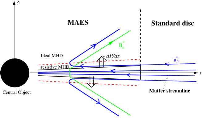
1.4 The MAES paradigm

A large scale (mean) magnetic field of bipolar topology is assumed to thread an accretion disc, allowing ejected plasma to flow along open field lines. This field extracts both angular momentum and energy from the underlying disc and transfers them back to the ejected plasma. There have been numerous studies of magnetized jets (e.g. Blandford & Payne 1982, Heyvaerts & Norman 1989, Pelletier & Pudritz 1992, Contopoulos & Lovelace 1994, Rosso & Pelletier 1994, Lery et al. 1999 to cite only a few), but they all suppose that the underlying disc would support the jets. In all these works, the disc itself was treated as a boundary condition, people usually assuming a standard viscous accretion disc (Shakura & Sunyaev 1973). However, if jets are to carry away the disc angular momentum, they strongly influence the disc dynamics.

The investigation of MAES, where accretion and ejection are interdependent, requires a new theory of accretion discs. The relevant questions that must be addressed by any realistic model of stationary magnetized accretion-ejection structures are the following:

(1) What are the relevant physical mechanisms inside the disc ?

(2) What are the physical conditions allowing accretion and ejection ?

(3) Can we relate jet properties to those of the disc ?

To answer these questions, one must take into account the full 2D problem (not 3D, thanks to axisymmetry) and not treat the disc as infinitely thin as in a standard disc theory. As a consequence, no toy-model has been able yet to catch the main features of these accretion-ejection structures. There, the disc accretion rate exhibits a radial variation as matter is being ejected. The link between accretion and ejection in a MAES can therefore be measured by the quantity $\xi=\frac{d\ln\dot{M}_{a}}{d\ln r}$ called the “ejection index”. This parameter (which can vary in the disc) measures a local ejection efficiency. In a standard accretion disc, $\xi=0$ everywhere leading to a constant accretion rate. A complete theory of MAES must provide the allowed values of $\xi$ as a function of the disc properties.

2 Theoretical framework of MAES

2.1 A magnetostatic approach

2.1.1 The Barlow experiment

A wheel made of a conducting material is put between the two poles of an electromagnet. This device produces a magnetic field perpendicular to the disc, along its axis of rotation. The wheel brushes against mercury contained in a tank, thereby allowing to close an electric circuit (mercury, wire connecting the disc axis, the disc itself). In order to check if some current is flowing, we can put a small lamp. With a crank, we then provide a rotating motion to the disc and let it evolve. If the magnetic field is off, nothing happens: the lamp stays mute (no current) and the disc very gradually slows down. On the contrary, if the magnetic field is present, the lamp lights on (a current is flowing) and the disc stops very quickly ! When the disc is finally motionless, the lamp is also off.

The explanation of this phenomenon lies in electromagnetic induction. The disc is made of a conducting material, meaning that charged particules are free to move inside it. When the disc starts to rotate, these particules drag the magnetic field along with them. The field lines become then twisted, showing a conversion of mechanical into magnetic energy. Once the disc has stopped, all the initial mechanical energy has been converted (here, dissipated into heat along the whole electric circuit). The magnetic field was just a mediator between different energy reservoirs.

2.1.2 On the importance of currents

A MAES is an astrophysical Barlow wheel. Indeed, the rotation of a conducting material in a static magnetic field $B_{z}$ induces an electric (more precisely electromotive) field

$$\vec{E}_{m}=\vec{u}\wedge\vec{B}\simeq\Omega rB_{z}\vec{e_{r}}$$ (1)

where $\Omega$ is the matter angular velocity and $\vec{e_{r}}$ the radial unit vector (in cylindrical coordinates). This field produces an electromotive force $e$, ie a difference of voltage between the inner $r_{i}$ and outer $r_{e}$ disc radii, namely

$$e=\int_{r_{i}}^{r_{e}}\vec{E}_{m}\cdot\vec{dr}\simeq\Omega_{i}r_{i}^{2}B_{i}$$ (2)

(where the dominant contribution is assumed to arise at the inner radius). In steady state, two electric circuits can develop (above and below the disc midplane) with a current $I_{\pm}=e/Z_{\pm}$ where $Z_{\pm}$ is their impedance. There is therefore an available electric power

$$P=e(I_{-}+I_{+})=\frac{\Omega_{i}^{2}r_{i}^{4}B_{i}^{2}}{Z_{eq}}$$ (3)

where $Z_{eq}$ is the equivalent impedance. Since a current $I=I_{-}+I_{+}$ is flowing inside the disc, it becomes affected by the magnetic field through the Laplace force $\vec{F}=\int_{r_{i}}^{r_{e}}I\vec{dr}\wedge\vec{B}$, which provides a torque acting against the disc rotation. This result is consistent with Lenz’s law, which states that induced currents work against the cause that gave birth to them.

Now, the existence of such a torque allows matter to fall towards the central engine, hence to be accreted. Energy conservation implies that the mechanical power liberated through accretion, namely

$$P_{acc}=\frac{GM\dot{M}_{a}}{2r_{i}}\ ,$$ (4)

where $\dot{M}_{a}$ is the accretion rate, must be equal to the electric power $P$. This imposes an impedance matching

$$Z_{eq}=\frac{2r_{i}^{2}B_{i}^{2}}{\dot{M}_{a}}\sim\mu_{o}\sqrt{\frac{GM}{r_{i}}}$$ (5)

where $\mu_{o}$ is the vacuum permeability. The rhs estimate used a magnetic field close to equipartition with the thermal energy inside the disc (see Sect 5.2.2). The disc accretion rate depends therefore on the global electric circuit.

Electric currents $I_{\pm}$ flow along the axis, more precisely are distributed inside the jets. But if we model such current as being carried by an electric wire, we can estimate the generated magnetic field, namely $B_{\phi}(r)=-\mu_{o}I/2\pi r$. Such a field is negative, consistent with the shear given by the disc rotation. Because of this field, there is a Laplace force towards the axis, ie the famous “hoop stress” which maintains the jets collimated.

To summarize:

1. Accretion: a torque due to the magnetic field extracts the disc angular momentum. Such a torque is related to the establishment of two parallel electric circuits. Their equivalent impedance is directly linked to the accretion rate affordable by the structure.

2. Global energy budget: a fraction of the accretion power is dissipated into Joule heating (disc and jets heating, allowing radiation), another is converted into kinetic power carried by the jets.

3. Jet acceleration: possible due to the conversion of electric into kinetic power. Note that if the impedances $Z_{+}$ and $Z_{-}$ (which describe all dissipative effects) are different, then two bipolar but asymmetric jets can be produced.

4. Jet collimation: jets do have naturally a self-collimating force if they carry a non-vanishing current. Since the electric circuit must be closed, not all magnetic field lines embrace a non-zero current. This obviously implies that all field lines anchored in the disc cannot be self-collimated (Okamoto 1999).

Lots of physics can be understood within the framework of magnetostatics. However, the precise description of a rotating astrophysical disc, its interrelations with outflowing plasma as well as the calculation of the asymptotic current distribution inside the jets (necessary to understand collimation) quite evidently require a fluid description.

2.2 Magnetohydrodynamics

Magnetohydrodynamics (MHD) describes the evolution of a collisional ionized gas (a plasma) submitted to the action of an electromagnetic field. Because the source of the field lies in the motions of charged particules (currents), the field is intrinsically tied to and dependent of these motions. Therefore, because of this high non-linearity, MHD offers an incredible amount of behaviours.

2.2.1 From a multicomponent to a single fluid description

Circumstellar discs and their associated jets are made of dust and gas, which is composed of different chemical species of neutrals, ions and electrons. We should therefore make a multicomponent treatment. However, this is far too complex especially when energetics comes in. On the other hand, if all components are well coupled (through collisions) a single fluid treatment becomes appropriate.

For each specie $\alpha$, we define its numerical density $n_{\alpha}$, mass $m_{\alpha}$, electric charge $q_{\alpha}$, velocity $\vec{v}_{\alpha}$ and pressure $P_{\alpha}$. The equation of motion for each specie writes

$$\rho_{\alpha}\frac{D\vec{v}_{\alpha}}{Dt}=-\vec{\nabla}P_{\alpha}-\rho_{\alpha}\vec{\nabla}\Phi_{G}+\sum_{\beta}\vec{F}_{\beta\alpha}+n_{\alpha}q_{\alpha}(\vec{E}+\vec{v}_{\alpha}\wedge\vec{B})$$ (6)

where $D./Dt=\partial./\partial t+\vec{v}_{\alpha}\cdot\nabla$ is the Lagrangean derivative, $\rho_{\alpha}=n_{\alpha}m_{\alpha}$, $\Phi_{G}$ is the gravitational potential of the central star and $\vec{F}_{\beta\alpha}$ is the collisional force due to all other species $\beta$. We can define the “mean” flow very naturally as

$$\rho = \sum_{\alpha}n_{\alpha}m_{\alpha}$$

$$\rho\vec{u} = \sum_{\alpha}m_{\alpha}n_{\alpha}\vec{v}_{\alpha}$$

$$P = \sum_{\alpha}n_{\alpha}k_{B}T$$ (7)

$$\vec{J} = \sum_{\alpha}n_{\alpha}q_{\alpha}\vec{v}_{\alpha}$$

where $\rho$ is the density, $\vec{u}$ the velocity, $P$ the pressure, $\vec{J}$ the current density and $k_{B}$ the Boltzmann constant. A single fluid description becomes relevant whenever the plasma is enough collisional. In such a case, we can safely assume that all species share the same temperature $T$. Moreover, we assume that any drift between the mean flow and a specie $\alpha$ is negligible, namely $\|\vec{v}_{\alpha}-\vec{u}\|\ll\|\vec{u}\|$. Using Newton’s second law ($\sum_{\alpha,\beta}\vec{F}_{\alpha\beta}=\vec{0}$) and local electrical neutrality ($\sum_{\alpha}n_{\alpha}q_{\alpha}=0$), we get the usual dynamical equations for one fluid

$$\frac{\partial\rho}{\partial t} + \nabla\cdot\rho\vec{u}=0$$ (8)

$$\rho\frac{D\vec{u}}{Dt} = -\nabla P-\rho\nabla\Phi_{G}+\vec{J}\wedge\vec{B}$$ (9)

by summing over all species $\alpha$. Even if the bulk of the flow is made of neutrals, they feel the magnetic force through collisions with ions (mainly) and electrons, $\vec{J}\wedge\vec{B}=(1+X)(\vec{F}_{in}+\vec{F}_{en})$ where $X=\rho_{i}/\rho_{n}$ is the density ratio of ions to neutrals.

The evolution of the electromagnetic field is described by Maxwell’s equations, namely (in vacuum)

$$\nabla\cdot\vec{B} = 0$$ (10)

$$\nabla\wedge\vec{B} = \mu_{o}\vec{J}+\frac{1}{c^{2}}\frac{\partial\vec{E}}{\partial t}$$ (11)

$$\nabla\cdot\vec{E} = \frac{\rho_{*}}{\varepsilon_{o}}$$ (12)

$$\nabla\wedge\vec{E} = -\frac{\partial\vec{B}}{\partial t}$$ (13)

Faraday’s law (Eq. 13) shows that the strength of the electric field varies like $E/B\sim L/t\sim U$ where $U$ is a typical plasma velocity. Now, using Ampère’s equation (11), shows that the displacement current has an effect of order $(U/c)^{2}$ only with respect to real currents ($c$ is the speed of light). Thus, in a non-relativistic plasma, it can be neglected providing a current density

$$\vec{J}=\frac{1}{\mu_{o}}\nabla\wedge\vec{B}$$ (14)

directly related to the magnetic field. Under this approximation, electric charge conservation

$$\frac{\partial\rho_{*}}{\partial t}+\nabla\cdot\vec{J}=0$$ (15)

shows that no charge accumulation is allowed: the first term is also of order $(U/c)^{2}$. Therefore $\nabla\cdot\vec{J}=0$, implying closed electric circuits.

Energy conservation of the electromagnetic field writes

$$\frac{\partial W}{\partial t}+\nabla\cdot\vec{S}_{MHD}=-\vec{J}\cdot\vec{E}$$ (16)

where $W=W_{e}+W_{m}=\varepsilon_{o}E^{2}/2+B^{2}/2\mu_{o}$ is the electromagnetic field energy density and

$$\vec{S}_{MHD}=\frac{\vec{E}\wedge\vec{B}}{\mu_{o}}$$ (17)

is the Poynting vector, carrying the field energy remaining after interaction with the plasma (the term $\vec{J}\cdot\vec{E}$). Inside the non-relativistic framework, the energy density contained in the electric field is negligible with respect to $W_{m}$ (of order $(U/c)^{2}$).

2.2.2 Generalized Ohm’s law

In order to close the above system of equations, we need to know the electric field $\vec{E}$. Its’ expression is obtained from the electrons momentum equation, consistently with the single fluid approximation. Namely, we assume that electrons are so light that they react almost instantaneously to any force, i.e.

$$\vec{0}=-\nabla P_{e} + \sum_{\beta}\vec{F}_{\beta e}-en_{e}(\vec{E}+\vec{v}_{e}\wedge\vec{B})$$ (18)

$$\vec{E}+\vec{u}\wedge\vec{B} = (\vec{u}-\vec{v}_{e})\wedge\vec{B}-\frac{\nabla P_{e}}{en_{e}}+\sum_{\beta}\frac{m_{\beta}n_{\beta}}{en_{e}}(\vec{v}_{\beta}-\vec{v}_{e})$$ (19)

Now, using (i) the expression of the Lorentz force $\vec{J}\wedge\vec{B}$, (ii) the approximation $\vec{J}\simeq en_{e}(\vec{v}_{i}-\vec{v}_{e})$ and (iii) neglecting the contribution due to the collisions between electrons and neutrals (with respect to those involving ions), we obtain the generalized Ohm’s law

$$\vec{E}\ +\ \vec{u}\wedge\vec{B}=\eta\vec{J}\ +\ \frac{\vec{J}\wedge\vec{B}}{en_{e}}\ -\ \left(\frac{\rho_{n}}{\rho}\right)^{2}\frac{(\vec{J}\wedge\vec{B})\wedge\vec{B}}{m_{in}n_{i}\nu_{in}}\ -\ \frac{\nabla P_{e}}{en_{e}}$$ (20)

where $\eta=(m_{ne}n_{n}\nu_{ne}+m_{ie}n_{i}\nu_{ie})/(en_{e})^{2}$ is the electrical (normal) resistivity due to collisions, and $m_{\alpha\beta}$ the reduced mass. The first term on the rhs is the Ohm term, the second is the Hall effect, the third the ambipolar diffusion term and the fourth a source of electric field due to any gradient of electronic pressure. Fortunately, all these terms become negligible with respect to $\vec{u}\wedge\vec{B}$ whenever the plasma is well coupled and ionized ($\rho_{n}\ll\rho$).

2.2.3 Plasma energy equation

This is the trickiest equation and can be written in several forms. We choose to express the internal energy equation, which can be written as

$$\rho T\frac{DS}{Dt}=\Gamma-\Lambda$$ (21)

where $S$ is the plasma specific entropy, $\Gamma$ all heating terms and $\Lambda$ all cooling terms. Note that a transport term (eg. such as conduction) can cool the plasma somewhere and heat it elsewhere. The MHD heating rate due to the interaction between the plasma and the electromagnetic field writes

$$\Gamma_{MHD}=\vec{J}\cdot(\vec{E}+\vec{u}\wedge\vec{B})\simeq\eta J^{2}+\left(\frac{\rho_{n}}{\rho}\right)^{2}\frac{\left|\vec{J}\wedge\vec{B}\right|^{2}}{m_{in}n_{i}\nu_{in}}$$ (22)

The first term is the Joule effect while the second is the heating due to ambipolar diffusion. Note that, although dynamically negligible in discs, such an effect might be responsible for jets heating (Safier 1993, Garcia et al. submitted).

2.3 Modelling a MAES

2.3.1 Assumptions

Our goal is to describe an accretion disc threaded by a large scale magnetic field of bipolar topology. In order to tackle this problem, we will make several symplifing assumptions:

(i) Single-fluid MHD: matter is ionized enough and all species well coupled. As a consequence, we use the simple form of Ohm’s law

$$\vec{E}+\vec{u}\wedge\vec{B}=\eta\vec{J}$$ (23)

Taking the curl of this equation and using Faraday’s law, we get the induction equation providing the time evolution of the magnetic field

$$\frac{\partial\vec{B}}{\partial t}=\nabla\wedge(\vec{u}\wedge\vec{B})-\nabla\wedge(\nu\nabla\wedge\vec{B})$$ (24)

where $\nu=\eta/\mu_{o}$ is the magnetic diffusivity. The first term describes the effect of advection of the field by the flow while the second describes the effect of diffusion, matter being able to cross field lines thanks to diffusivity.

(ii) Axisymmetry: using cylindrical coordinates ($r$, $\phi$, $z$) no quantity depends on $\phi$, the jet axis being the vertical axis. As a consequence $E_{\phi}=0$ and all quantities can be decomposed into poloidal (the ($r$, $z$) plane) and toroidal components, eg. $\vec{u}=\vec{u_{p}}+\Omega r\vec{e_{\phi}}$ and $\vec{B}=\vec{B_{p}}+B_{\phi}\vec{e_{\phi}}$. A bipolar magnetic configuration can then be described with

$$\vec{B_{p}}=\frac{1}{r}\nabla a\wedge\vec{e_{\phi}}\ ,$$ (25)

where $a(r,z)$ is an even function of $z$ and with an odd toroidal field $B_{\phi}(r,-z)=-B_{\phi}(r,r)$. The flux function $a$ is related to the toroidal component of the potential vector ($a=rA_{\phi}$) and $a(r,z)=constant$ describes a surface of constant vertical magnetic flux $\Phi$,

$$\Phi=\int_{S}\vec{B}\cdot\vec{dS}=2\pi a(r,z)\ .$$ (26)

The magnetic field distribution in the disc as well as the total amount of flux are unknown and must therefore be prescribed.

(iii) Steady-state: all astrophysical jets display proper motions and/or emission nodules, showing that they are either prone to some instabilities or that ejection is an intermittent process. However, the time scales involved in all objects are always much larger than the dynamical time scale of the underlying accretion disc. Therefore, a steady state approach is appropriate.

(iv) Transport coefficients: if we use a normal (collisional) value for $\nu$, we find that the ratio of advection to diffusion in (24), measured by the magnetic Reynolds number

$${\cal R}_{m}\sim\frac{LU}{\nu}\ ,$$ (27)

is always much larger than unity inside both the disc and the jets. This is the limit of ideal MHD where plasma and magnetic fields are “frozen in”. Jets are therefore described with ideal MHD ($\eta=0$). Within this framework, the stronger (initially the magnetic field) carries the weaker (ejected disc plasma) along with it. But inside the disc, gravitation is the dominant energy source and the plasma drags and winds up the field lines. Such a situation cannot be maintained for very long. Instabilities of different kind will certainly be triggered leading to some kind of saturated, turbulent, disc state (eg. tearing mode instabilities, or magneto-rotational instability, Balbus & Hawley 1991).

In turbulent media, all transport effects are enhanced, leading to anomalous transport coefficients. These coefficients are the magnetic diffusivity $\nu_{m}$ and resistivity $\eta_{m}$, but also the viscosity $\nu_{v}$ (associated with the transport of momentum) and thermal conductivity $\kappa_{T}$ (associated with the heat flux). Providing the expressions of these anomalous coefficients requires a theory of MHD turbulence inside accretion discs. Having no theory, we will use simple prescriptions, like the alpha prescription used by Shakura & Sunyaev (1973). In particular, because of the dominant Keplerian motion in discs, we allow for a possible anisotropy of the magnetic diffusivity. Namely, we use two different turbulent diffusivities: $\nu_{m}$ (related to the diffusion in the ($r$, $z$) plane) and $\nu^{\prime}_{m}$ (related to the diffusion in the $\phi$ direction).

Since stationary discs must be turbulent, all fields (eg. velocity, magnetic field) must be understood now in some time average sense.

(v) Non-relativistic MHD framework: in YSOs, matter remains always non-relativistic but there is something more about it. Indeed, magnetic field lines are anchored in an rotating accretion disc. Hence, if a field line of angular velocity $\Omega_{*}$ opens a lot, there is a cylindrical distance such that its linear velocity reaches the speed of light, defining a “light cylinder” $R_{L}=c/\Omega_{*}$. Now, if one imposes ideal MHD regime along the jet, ie. $\vec{E}=-\vec{u}\wedge\vec{B}=-\Omega_{*}r\vec{e_{\phi}}\wedge\vec{B_{p}}$, we see that the displacement current is no longer negligible at the light cylinder: propagation effects become relevant and one must take into account a local non-zero electric charge $\rho_{*}$ (provided by the Goldreich-Julian charge $\nabla\cdot\vec{E}=\rho_{*}/\varepsilon_{o}$). As a consequence, the plasma feels an additional electric force $\rho_{*}\vec{E}$, even if the bulk velocity of the flow is non relativistic (eg. Breitmoser & Camenzind 2000)!

But remember that this extra force and its corresponding “light cylinder” arose because of the assumption of ideal MHD. In fact, taking into account a local charge density probably imposes to also treat the non-ideal contributions (see Eq. 20). Nobody provided yet a self-consistent calculation. We just assume here that any charge accumulation would be quickly canceled (no dynamical relevance of the light cylinder).

2.3.2 Set of MHD equations

We use the following set of MHD equations:

Mass conservation

$$\nabla\cdot\rho\vec{u}=0$$ (28)

Momentum conservation

$$\rho\vec{u}\cdot\nabla\vec{u}=-\nabla P-\rho\nabla\Phi_{G}+\vec{J}\wedge\vec{B}+\nabla\cdot{\mathsf{T}}$$ (29)

where $\mu_{o}\vec{J}=\nabla\wedge\vec{B}$ is the current density and ${\mathsf{T}}$ the turbulent stress tensorm which is related to the turbulent viscosity $\nu_{v}$ (Shakura & Sunyaev 1973).

Ohm’s law and toroidal field induction

$$\eta_{m}\vec{J}_{\phi} = \vec{u_{p}}\wedge\vec{B_{p}}$$ (30)

$$\nabla\cdot(\frac{\nu^{\prime}_{m}}{r^{2}}\nabla rB_{\phi}) = \nabla\cdot\frac{1}{r}(B_{\phi}\vec{u_{p}}-\vec{B_{p}}\Omega r)$$ (31)

where $\eta_{m}=\mu_{o}\nu_{m}$ and $\eta^{\prime}_{m}=\mu_{o}\nu^{\prime}_{m}$ are the anomalous resistivities.

Perfect gas law

$$P=\rho\frac{k_{B}}{\mu m_{p}}T$$ (32)

where $m_{p}$ is the proton mass and $\mu$ a generalized “mean molecular weight”.

Energy equation
As seen previously, the exact energy equation (21) involves various physical mechanisms. Its explicit form is

$$\nabla\cdot(U\vec{u_{p}}\ +\ \vec{S}_{rad}\ +\ \vec{q}_{turb})=-P\nabla\cdot\vec{u_{p}}\ +\ \eta_{m}J^{2}_{\phi}\ +\ \eta^{\prime}_{m}J^{2}_{p}\ +\ \eta_{v}\left|r\nabla\Omega\right|^{2}$$ (33)

where $\eta_{v}=\rho\nu_{v}$, $U$ is the internal specific energy, $\vec{S}_{rad}=-\frac{c}{\kappa\rho}\nabla P_{rad}$ is the radiative energy flux ($\kappa$ is the Rosseland mean opacity of the plasma, $P_{rad}$ the radiation pressure) and $\vec{q}_{turb}$ the unknown turbulent energy flux. This flux of energy arises from turbulent motions and provides both a local cooling $\Lambda_{turb}$ and heating $\Gamma_{turb}$. Indeed, using a kinetic description and allowing for fluctuations in the plasma velocity and magnetic field, it is possible to show that all energetic effects associated with these fluctuations cannot be reduced to only anomalous Joule and viscous heating terms. Therefore, a consistent treatment of turbulence imposes to take into account $\vec{q}_{turb}$ (see early paper of Shakura et al. 1978). But how to do it ? Moreover, the radiative flux depends on the local opacity $\kappa$ of the plasma, which varies both radially and vertically inside the disc. Besides, the expression of the radiative pressure $P_{rad}$ is known only in optically thick media ($P_{rad}=aT^{4}$), while the disc can be already optically thin at the disc midplane.

Thus, it seems that a realistic treatment of the energy equation is still out of range. As a first step to minimize its impact on the whole structure, we will use a polytropic equation

$$P=K\rho^{\Gamma}\ ,$$ (34)

where the polytropic index $\Gamma$ can be set to vary between 1 (isothermal case) and $\gamma=\frac{5}{3}$ (adiabatic case) for a monoatomic gas. Here $K$ can be allowed to vary radially but remains constant along each field line. In section 5.3, we will turn our attention to thermal effects and use therefore a more appropriate form of the energy equation.

Using the above set of MHD equations to describe astrophysical discs and jets would normally require consistency checks, at least a posteriori. If one fluid MHD seems justified inside the inner regions of accretion discs, it may well not be anymore the case along the jet (huge fall in density). In particular non-ideal effects are most probably starting to play a role in Ohm’s law (ambipolar diffusion or even Hall terms), allowing matter to slowly drift across field lines. This may have important dynamical effects dowstream. To clearly settle this question, the full thermodynamics of the plasma including its ionization state should be self-consistently solved along the jet.

2.4 Critical points in stationary flows

In the real world, everything is time dependent. Imagine matter expelled from the disc without the required energy: it will fall down, thereby modifying the conditions of ejection. A steady state is eventually reached after a time related to the nature of the waves travelling upstream and providing the disc information on what’s going on further up.

The adjustment of a MAES corresponds to the phenomenon of impedance matching. As we saw, this matching relates the accretion rate to the dissipative effects in the electric circuit. In practice, this means that the resolution of stationary flows requires to take into account, in some way, all time-dependent feedback mechanisms. This is done by requiring that, once a steady-state is achieved, no information (ie. no waves) can propagate upstream, from infinity (in the z-direction) to the accretion disc. There is only one way to do it. Matter must flow faster than any wave, leaving the disc causally disconnected from its surroundings.

2.4.1 The Parker wind

Let us first look at the simple model of a spherically symmetric, isothermal, hydrodynamic flow. Such a model was first proposed by Parker (1958) to explain the solar wind. In spherical coordinates, mass conservation and momentum conservation write

$$\frac{du}{u}+\frac{d\rho}{\rho}+2\frac{dr}{r} = 0$$ (35)

$$u\frac{du}{dr}+\frac{1}{\rho}\frac{dP}{dr}+\frac{GM}{r^{2}} = 0$$ (36)

where gas pressure is $P=\rho C_{s}^{2}$, the sound speed $C_{s}$ being a constant. In such a simple system is hidden a singularity. Indeed, after differentiation one gets

$$(C_{s}^{2}-u^{2})\frac{d\ln\rho}{dr} = 2\frac{u^{2}}{r}-\frac{GM}{r^{2}}$$ (37)

$$(C_{s}^{2}-u^{2})\frac{d\ln u}{dr} = -2\frac{C_{s}^{2}}{r}+\frac{GM}{r^{2}}$$ (38)

showing that the system is singular at $r=r_{s}$, where $u=C_{s}$. In order to obtain a stationary solution, one must then impose the regularity condition which is

$$r_{s}=\frac{GM}{2C_{s}^{2}}$$ (39)

In practice, fixing the distance of the sonic point imposes the value of one free parameter (eg. the initial velocity or density). Only the trans-sonic solution is stationary.

2.4.2 Critical points of a MAES

In a magnetized medium, there are several waves able to transport information, related to the different restoring forces. In a MAES, the Lorentz force couples with the plasma pressure gradient leading to three different MHD waves:

• the Alfvén wave (A), causing only magnetic disturbances along the unperturbed magnetic field $B_{o}$ and of phase velocity

  $$V_{A}=\frac{B_{o}}{\sqrt{\mu_{o}\rho}}$$

• two magnetosonic waves, the slow (SM) and the fast (FM), involving both magnetic disturbances and plasma compression (rarefaction), of phase velocity

  $$V^{2}_{SM,FM}=\frac{1}{2}\left(V_{A}^{2}+C_{s}^{2}\mp\sqrt{(V_{A}^{2}+C_{S}^{2})^{2}-4V_{A}^{2}C_{s}^{2}\cos^{2}\theta}\right)$$

  where $\theta$ is the angle between the unperturbed field $B_{o}$ and the direction of propagation of the wave (the disturbance).

In ideal MHD regime (in the jets), these three waves can freely propagate. This provides three singularities along each magnetic surface, whenever the plasma velocity equals one of these phase speeds. Thus, three regularity conditions must be specified per magnetic surface.

Inside the turbulent accretion disc it is another story. There, the high level of turbulence maintains large magnetic diffusivities and viscosity. As a result, MHD waves are strongly damped and the number of singularities really present is not so clear. Within the alpha prescription of accretion discs (Shakura & Sunyaev 1973), viscosity appears only in the azimuthal equation of motion (angular momentum conservation). The presence of viscosity there “damps” the acoustic waves and there is no singularity related to this motion (although rotation is supersonic). Conversely, there is no viscosity in the poloidal (radial and vertical) equations of motion: a singularity can therefore appear there, related to pure acoustic waves. As a consequence, in principle, it may be necessary to impose a regularity condition with respect to the accretion flow itself, if it becomes supersonic.

3 Magnetized jets

3.1 Commonly used equations

As said previously, jets are in ideal MHD regime, namely $\nu_{v}=\nu_{m}=\nu^{\prime}_{m}=0$. In this regime, mass and flux conservations combined with Ohm’s law (30) provide

$$\vec{u}_{p}=\frac{\eta(a)}{\mu_{o}\rho}\vec{B}_{p}$$ (40)

where $\eta(a)=\sqrt{\mu_{o}\rho_{A}}$ is a constant along a magnetic surface and $\rho_{A}$ is the density at the Alfvén point, where the poloidal velocity $u_{p}$ reaches the poloidal Alfvén velocity $V_{Ap}$. The induction equation (31) becomes

$$\Omega_{*}(a)=\Omega-\eta\frac{B_{\phi}}{\mu_{o}\rho r}\ ,$$ (41)

where $\Omega_{*}(a)$ is the rotation rate of a magnetic surface (imposed by the disc, thus very close to the Keplerian value). Note that despite the frozen in situation, jet plasma flows along a magnetic surface with a total velocity $\vec{u}=(\eta/\mu_{o}\rho)\vec{B}\ +\ \Omega_{*}r\vec{e_{\phi}}$ which is not parallel to the total magnetic field $\vec{B}$. This is possible because field lines rotate faster than the ejected plasma. If the disc is rotating counter-clockwise, the field lines will be trailing spirals ($\Omega_{*}>\Omega$, ie. $B_{\phi}<0$ with $B_{z}>0$), while ejected plasma will rotate in the same direction as in the disc. Magnetic field lines and plasma stremlines are thus two helices of different twist. Jet angular momentum conservation simply writes

$$\Omega_{*}r^{2}_{A}=\Omega r^{2}-\frac{rB_{\phi}}{\eta}$$ (42)

where $r_{A}$ is the Alfvén radius. Above the disc, the turbulent torque vanishes and only remains a magnetic accelerating torque. The first term on rhs is the specific angular momentum carried by the ejected plasma whereas the last tern can be understood as the angular momentum stored in the magnetic field. The total specific angular momentum $L(a)=\Omega_{*}r^{2}_{A}$ is an MHD invariant. The Alfvén radius $r_{A}$ can be interpretated as a magnetic lever arm, braking down the disc. The larger the ratio $r_{A}/r_{o}$, the larger the magnetic torque acting on the disc at the radius $r_{o}$.

Hereafter, we focus only on adiabatic jets (for which thermal effects can still be non negligible). Usually, instead of using the other two components of the momentum conservation equation, one uses the Bernoulli equation (obtained by projecting Eq. (29) along the poloidal direction, ie. $\vec{B}_{p}$) and the transverse field or Grad-Shafranov equation (obtained, after quite a lot of algebra, by projecting Eq. (29) in the direction perpendicular to a magnetic surface, ie. $\nabla a$). For a jet of adiabatic index $\gamma$, Bernoulli equation writes

$$E(a)=\frac{u^{2}}{2}+H+\Phi_{G}-\Omega_{*}r\frac{B_{\phi}}{\sqrt{\mu_{o}\rho_{A}}}$$ (43)

where $u$ is the total plasma velocity and $H=(\gamma/\gamma-1)P/\rho$ is the gas enthalpy. This equation describes the acceleration of matter along a poloidal magnetic surface, namely the conversion of magnetic energy and enthalpy into ordered kinetic energy. Grad-Shafranov equation of an adiabatic jet is

$$\nabla\cdot(m^{2}-1)\frac{\nabla a}{\mu_{o}r^{2}} = \rho\left\{\frac{dE}{da}-\Omega\frac{d\Omega_{*}r_{A}^{2}}{da}\right.\ +\ \left.(\Omega r^{2}-\Omega_{*}r^{2}_{A})\frac{d\Omega_{*}}{da}\ -\ \frac{C_{s}^{2}}{\gamma(\gamma-1)}\frac{d\ln K}{da}\right\}$$ (44)

$$\ +\ \frac{B^{2}_{\phi}+m^{2}B^{2}_{p}}{\mu_{o}}\frac{d\ln\eta}{da}$$

where $m^{2}\equiv u^{2}_{p}/V^{2}_{Ap}$ is the Alfvénic Mach number and $C_{s}^{2}=\gamma k_{B}T/\mu m_{p}$ is the jet sound speed. This awful equation provides the transverse equilibrium (ie. the degree of collimation) of a magnetic surface. A simpler-to-use and equivalent version of this equation is

$$(1-m^{2})\frac{B^{2}_{p}}{\mu_{o}{\cal R}}\ -\ \nabla_{\perp}\left(P+\frac{B^{2}}{2\mu_{o}}\right)\ -\ \rho\nabla_{\perp}\Phi_{G}\ +\ (\rho\Omega^{2}r-\frac{B^{2}_{\phi}}{\mu_{o}r})\nabla_{\perp}r=0$$ (45)

where $\nabla_{\perp}\equiv\nabla a\cdot\nabla/|\nabla a|$ provides the gradient of a quantity perpendicular to a magnetic surface ($\nabla_{\perp}Q<0$ for a quantity $Q$ decreasing with increasing magnetic flux) and ${\cal R}$, defined by

$$\frac{1}{{\cal R}}\equiv\frac{\nabla a}{|\nabla a|}\cdot\frac{(\vec{B}_{p}\cdot\nabla)\vec{B}_{p}}{B^{2}_{p}}\ ,$$ (46)

is the local curvature radius of a particular magnetic surface. When ${\cal R}>0$, the surface is bent outwardly while for ${\cal R}<0$, it bends inwardly. The first term in Eq.(45) describes the reaction to the other forces of both magnetic tension due to the magnetic surface (with the sign of the curvature radius) and inertia of matter flowing along it (hence with opposite sign). The other forces are the total pressure gradient, gravity (which acts to close the surfaces and deccelerate the flow, but whose effect is already negligible at the Alfvén surface), and the centrifugal outward effect competing with the inwards hoop-stress due to the toroidal field.

To summarize, an astrophysical jet is a bunch of axisymmetric magnetic surfaces $a(r,z)=Const.$, nested one around the other at different anchoring radii $r_{o}$. The magnetic flux distribution $a(r_{o})$ is unknown and is therefore prescribed, whereas the shape $r(z)$ of the magnetic surface is self-consistently calculated. Each magnetic surface is characterized by 5 MHD invariants:

- $\eta(a)$, ratio of ejected mass flux to magnetic flux;

- $\Omega_{*}(a)$, the rotation rate of the magnetic surface;

- $L(a)=\Omega_{*}r_{A}^{2}$, the total specific angular momentum transported;

- $E(a)$, the total specific energy carried away;

- $K(a)$, related to the specific entropy $S(a)$.

A magnetized jet is then described by 8 unknown variables: density $\rho$, velocity $\vec{u}$, magnetic field $\vec{B}$ (flux function $a$ and toroidal field $B_{\phi}$), pressure $P$ and temperature $T$. There are 8 equations allowing us to solve the complete problem: (25), (32), (34), (40), (41), (42), (43) and (44) or its more physically meaningful version (45). Since the ejected plasma must become super-FM, 3 regularity conditions have to be imposed, leaving the problem with 5 free boundary conditions (at each radius $r_{o}$). Studies of disc-driven jets usually assume that matter rotates at the Keplerian speed, namely $\Omega_{o}=\Omega_{K}(r_{o})=\sqrt{GM/r_{o}^{3}}$ and that jets are “cold” (negligible enthalpy, $K(a)=0$) or choose an arbitrary distribution $K(a)$. In both cases, it leaves the problem with only 3 free and independent boundary conditions that must be specified at each radius.

Magnetized jets are such complicated objects that only gross properties are known. For example, we know that a non-vanishing asymptotic current will produce a self-confinement of some field lines (Heyvaerts & Norman 1989). But the exact proportion of collimated field lines depends on “details” (transverse gradients of inner properties, outer pressure). The distance at which jets become collimated, the jet radius and opening angle, the velocity and density transverse distributions still remain to be found in full generality. This is the reason why there are so many different works on jet dynamics and why each authors use their own “relevant” parameters. Following Blandford & Payne (1982), we introduce the following jet parameters

$$\lambda = \frac{\Omega_{*}r^{2}_{A}}{\Omega_{o}r^{2}_{o}}\simeq\frac{r^{2}_{A}}{r^{2}_{o}}\simeq 1-\frac{B_{\phi}^{+}}{\eta\Omega_{o}r_{o}}$$

$$\kappa = \eta\frac{\Omega_{o}r_{o}}{B_{o}}\simeq\frac{\mu_{o}\Omega_{o}r_{o}}{B_{o}^{2}}\rho^{+}u_{z}^{+}$$ (47)

The index “o” refers to quantities evaluated at the disc midplane, “+” at the disc surface and “A” at the Alfvén point. The first parameter, $\lambda$, is a measure of the magnetic lever arm that brakes down the disc while $\kappa$ measures the ejected mass flux. Another parameter is usually introduced, related somehow to the jet asymptotic behaviour. We use

$$\omega_{A}=\frac{\Omega_{*}r_{A}}{V_{Ap,A}}\simeq\kappa\lambda^{1/2}\frac{B_{o}}{B_{p,A}}$$ (48)

which measures the ratio of the rotational velocity to the poloidal jet velocity at the Alfvén point. Such a parameter characterises the magnetic rotator: cold jets require $\omega_{A}>1$ to become trans-Alfvénic (Pelletier & Pudritz 1992, Ferreira 1997, Lery et al. 1999). Note also that its value depends on pure geometrical effects, namely the way the magnetic surface opens. As a consequence, spherical expansion of field lines is probably a special case, leading to particular relations between jet asymptotic behaviour and its source.

3.2 Some aspects of cold jets physics

3.2.1 Energetic requirements

It is quite reasonable to assume that the magnetic energy density in the disc is much smaller than the gravitational energy density. As a consequence, the rotation of the disc drags the magnetic field lines which become then twisted. This conversion of mechanical to magnetic energy in the disc gives rise to an outward poloidal MHD Poynting flux

$$\vec{S}_{MHD,p}=\frac{\vec{E}\times\vec{B}_{\phi}}{\mu_{o}}=-\Omega_{*}rB_{\phi}\frac{\vec{B}_{p}}{\mu_{o}}$$ (49)

which feeds the jets and appears as the magnetic term in the Bernoulli integral (43). Another source of energy for the jet could be the enthalpy $H$ (built up inside the disc and advected by the ejected flow) or another local source of heating ${\cal Q}$ (eg. coronal heating). We are mainly interested here in “cold” jets, where those two terms are negligible (see Sect. 5.3). Bernoulli equation can be rewritten as

$$E(a)=\frac{u_{p}^{2}}{2}\ +\ \Phi_{eff}\ +\ H$$ (50)

where the effective potential is $\Phi_{eff}=\Phi_{G}-\frac{1-g^{2}}{2}\Omega_{*}^{2}r^{2}$ with $\Omega=\Omega_{*}(1-g)$ and $\Omega_{*}\simeq\Omega_{o}$. The function $g$ is much smaller than unity at the disc surface then increases along the jet (if the jet widens a lot, $g\rightarrow 1$). Starting from a point located at the disc surface $(r_{o},z=0)$, matter follows along a magnetic surface and must move to another point $(r_{o}+\delta r_{o},z)$. This can be done only if a positive poloidal velocity is indeed developed. Making a Taylor expansion of $\Phi_{eff}$, one gets $\frac{u_{p}^{2}}{2}\simeq H_{o}-H+\frac{\Omega_{o}^{2}}{2}(3\delta r_{o}^{2}-z^{2})>0$, which translates into the condition

$$\tan\theta=\frac{z}{\delta r_{o}}<\sqrt{3}\left(1+\frac{2}{3}\frac{H_{o}-H}{\Omega_{o}^{2}\delta r_{o}^{2}}\right)^{1/2}\ .$$ (51)

Thus, cold jets (negligible enthalpy) require field lines bent by more than $30^{o}$ with respect to the vertical axis at the disc surface (Blandford & Payne 1982). The presence of a significant enthalpy ($H_{o}$ large) is obviously required if this condition is not satisfied. Bernoulli equation (43) gives a total energy feeding a cold jet

$$E(a)=\frac{\Omega_{o}^{2}r_{o}^{2}}{2}-\Omega_{o}^{2}r_{o}^{2}+\Omega_{*}(\Omega_{*}r_{A}^{2}-\Omega_{o}r_{o}^{2})=\frac{\Omega_{o}^{2}r_{o}^{2}}{2}(2\lambda-3)$$ (52)

which is directly controlled by the magnetic lever arm $\lambda$. Cold, super-FM jets require therefore $\lambda>3/2$. If all available energy is converted into kinetic energy, ejected plasma reaches an asymptotic poloidal velocity $u_{\infty}(a)=\sqrt{2E(a)}$.

3.2.2 Relevant forces and current distributions

So, rotation of open field lines produces a shear ($B^{+}_{\phi}<0$) that results in an outward flux of energy. Once matter is loaded onto these field lines, it will be flung out whenever there are forces overcoming the gravitational attraction. Since matter flows along magnetic surfaces, one must look at the projection of all forces along these surfaces. We obtain for the Lorentz force,

$$F_{\phi} = \frac{B_{p}}{2\pi r}\nabla_{\parallel}I$$

$$F_{\parallel} = -\frac{B_{\phi}}{2\pi r}\nabla_{\parallel}I$$ (53)

where $\nabla_{\parallel}=\vec{\nabla}\cdot\vec{B}_{p}/B_{p}$ and $I=2\pi rB_{\phi}/\mu_{o}$ is the total poloidal current flowing inside the magnetic surface. Hence, jets are magnetically-driven whenever $\nabla_{\parallel}I>0$ is fulfilled, namely when current is leaking through this surface. This quite obscur condition describes the fact that magnetic energy is being converted into kinetic energy: the field lines accelerate matter both azimuthaly ($F_{\phi}>0$) and along the magnetic surface ($F_{\parallel}>0$). The difference with the Barlow wheel lies in the possibility to convert magnetic energy into jet (bulk) kinetic energy.

The jet transverse equilibrium depends on the subtle interplay between several forces (see Eq. (45)). The transverse projection of the magnetic force, namely

$$F_{\perp}=B_{p}J_{\phi}-\frac{B_{\phi}}{2\pi r}\nabla_{\perp}I$$ (54)

where $\nabla_{\perp}\equiv(\nabla a\cdot\nabla)/|\nabla a|$, shows that it depends on the transverse current distribution. Thus, the degree of jet collimation (as well as plasma acceleration) depends on the overall electric current circuit. Any bias introduced on this circuit can produce an artificial force and modify diagnostics on jet collimation.

Eventually matter becomes no longer magnetically accelerated and $\nabla_{\parallel}I=0$ is satisfied. This implies two possible asymptotic current distributions. If jets are force-free (ie. $\vec{J}_{p}$ and $\vec{B}_{p}$ parallel), then there is a non-vanishing asymptotic current providing a self-collimating pinch (and one must worry about how the electric circuit is closed). Or, jets become asymptotically current-free ($I_{\infty}=0$) and another cause must then be responsible for their collimation (either inertial or external pressure confinement). This last alternative has something appealing for magnetic fields would then have a major influence only at the jet basis, becoming dynamically negligible asymptotically (cf Sect. 1.1).

3.3 Numerical simulations: what can be learned of them ?

There have been a lot of numerical studies of MHD jet propagation and their associated instabilities. Here, I focus only on those addressing the problem of jet formation from accretion discs. Although some attempts have been made to model accretion discs driving jets, difficulties are such that nothing realistic has been obtained yet (Shibata & Uchida 1985, Stone & Norman 1994, Kudoh et al. 1998). Ejection is indeed observed, but no one can tell whether these events are just transients or if they indeed represent some realistic situation.

Another philosophy is to treat the disc as a boundary condition and, starting from an (almost) arbitrary initial condition, wait until the system converges towards a stationary flow (Ustyugova et al. 1999, 2000, Ouyed & Pudritz 1997, 1999, Krasnopolsky et al. 1999). Now, it is of no wonder that jets are indeed obtained with these simulations. Matter, forced to flow along open magnetic field lines, is continuously injected (at a rate $\rho^{+}u^{+}_{z}$) at the bottom of the computational box. As a response, the field lines twist (ie. $B_{\phi}$ increases) until there is enough magnetic energy to propell it. If the code is robust enough, a steady-state situation is eventually reached, actually reproducing most of the results obtained with self-similar calculations (Krasnopolsky et al. 1999). Ouyed & Pudritz (1997) found a parameter region where unsteady solutions are produced, with a “knot generator” whose location seems to remain fixed. Their results may be related to the characteristic recollimation configuration featured by self-similar solutions (Blandford & Payne 1982, Contopoulos & Lovelace 1994, Ferreira 1997).

Nevertheless, since the time step for computation depends on the faster waves (Courant condition) whose phase speed varies like $\rho^{-1/2}$, it appears that no current MHD code can cope with tiny mass fluxes. Thus, code convergence itself introduces a bias in the mass flux of numerical jets. These are always very “heavy”, with a magnetic lever arm $r_{A}/r_{o}$ not even reaching 4 (Ouyed & Pudritz 1999, Krasnopolsky et al. 1999, Ustyugova et al. 1999) while cold self-similar studies obtained much larger values (with a minimum value around 10). This is not a limitation imposed by physics but of computers and will certainly be overcome in the future.

On the other hand, the question of jet collimation is clearly one that can be addressed by simulations. However, the boundary conditions imposed at the box, as well as the shape of the computational domain, can introduce artificial forces leading to unsteady jets or spurious collimation (see the nice paper of Ustyugova et al. 1999).

Anyway, the following crucial question remains to be addressed: how (and how much) matter is loaded into the field lines ? Or another way to put it: how is matter steadily deflected from its radial motion (accretion) to a vertical one (ejection) ? To answer this question one must treat the accretion disc in a self-consistent way.

4 Magnetized accretion discs driving jets

4.1 Physical processes in quasi-Keplerian discs

4.1.1 Turbulent, Keplerian discs

As said previously, we focus our study on Keplerian accretion discs. Such a restriction imposes negligible radial plasma pressure gradient and magnetic tension. We define the local vertical scale height as $P_{o}=\rho_{o}\Omega_{K}^{2}h^{2}$ where $P_{o}$ is the total plasma pressure. Looking at the disc radial equilibrium, a Keplerian rotation rate is indeed obtained whenever the disc aspect ratio

$$\varepsilon=\frac{h(r)}{r}$$ (55)

is smaller than unity. Hereafter, we use $\varepsilon<1$ as a free parameter and we will check a posteriori the thin disc approximation (Sect. 5.4.1).

Steady accretion requires a turbulent magnetic diffusivity for matter must cross field lines while accreting and rotating. Since rotation is much faster than accretion, there must be a higher dissipation of toroidal field than poloidal one. A priori, this implies a possible anisotropy of the magnetic diffusivities associated with these two directions, poloidal $\nu_{m}$ and toroidal $\nu_{m}^{\prime}$. Besides, such a turbulence might also provide a radial transport of angular momentum, hence an anomalous viscosity $\nu_{v}$. To summary, at least three anomalous transport coefficients are necessary to describe a stationary MAES. We will use the following dimensionless parameters defined at the disc midplane:

$$\alpha_{m}=\frac{\nu_{m}}{v_{A}h}$$ level of turbulence

$$\chi_{m}=\frac{\nu_{m}}{\nu_{m}^{\prime}}$$ degree of anisotropy (56)

$${\cal P}_{m}=\frac{\nu_{v}}{\nu_{m}}$$ magnetic Prandtl number

where $v_{A}=B_{o}/\sqrt{\mu_{o}\rho_{o}}$ is the Alfvén speed. Our conventional view of 3D turbulence would translate into $\alpha_{m}<1$, $\chi_{m}\sim 1$ and ${\cal P}_{m}\sim 1$. But as stated before, the amount of current dissipation may be much higher in the toroidal direction, leading to $\chi_{m}\ll 1$. Moreover, it is not obvious that $\alpha_{m}$ must necessarily be much smaller than unity. Indeed, stationarity requires that the time scale for a magnetic perturbation to propagate in the vertical direction, $h/v_{A}$, is longer than the dissipation time scale, $h^{2}/\nu_{m}$. This roughly translates into $\alpha_{m}>1$. Thus, we must be cautious and will freely scan the parameter space defined by these turbulence parameters.

4.1.2 How is accretion achieved ?

The disc being turbulent, accretion of matter bends the poloidal field lines whose steady configuration is provided by Ohm’s law (30). At the disc midplane, this equation provides

$${\cal R}_{m}\equiv\frac{ru_{o}}{\nu_{m}}=\left.\frac{\mu_{o}rJ_{\phi}}{B_{z}}\right|_{z=0}\sim\frac{l^{2}}{r^{2}}$$ (57)

where ${\cal R}_{m}$ is the magnetic Reynolds number related to the radial motion $u_{o}$ and $l(r)$ is the characteristic scale height of the magnetic flux variation. Once the disc turbulence properties are given, we just need to know the accretion velocity $u_{o}$. This is provided by the angular momentum equation, namely

$$\rho\frac{\vec{u}_{p}}{r}\cdot\nabla\Omega r^{2}=F_{\phi}+(\nabla\cdot{\mathsf{T}})\cdot\vec{e}_{\phi}$$ (58)

where $F_{\phi}$ is the magnetic torque due to the large scale magnetic field (“jet” torque) and $(\nabla\cdot{\mathsf{T}})\cdot\vec{e}_{\phi}$ is the “viscous”-like torque of turbulent origin (possibly due to the presence of a small scale magnetic field). Such an equation can be put into the following conservative form

$$\nabla\cdot\left[\rho\Omega r^{2}\vec{u}_{p}\ -\ \frac{rB_{\phi}}{\mu_{o}}\vec{B}_{p}\ -\ r\vec{T}_{v}\right]=0$$ (59)

where $r(\nabla\cdot{\mathsf{T}})\cdot\vec{e}_{\phi}=\nabla\cdot r\vec{T}_{v}$. Although modelling the jet torque is quite straightforward, it is not the case of the turbulent torque $\vec{T}_{v}$ and we use a prescription analogous to Shakura & Sunyaev (1973). Defining

$$\Lambda=\left|\frac{\mbox{jet torque}}{\mbox{turbulent torque}}\right|_{z=0}$$ (60)

the disc angular momentum conservation becomes at the disc midplane

$$1+\Lambda\simeq{\cal R}_{m}\left(\frac{\nu_{m}}{\nu_{v}}\right)=\frac{{\cal R}_{m}}{{\cal P}_{m}}$$ (61)

Taking the conventional value ${\cal P}_{m}\sim 1$, one sees that a “standard” accretion disc, which is dominated by the viscous torque ($\Lambda\ll 1$) requires straigth poloidal field lines (${\cal R}_{m}\sim 1$, Heyvaerts et al. 1996). On the contrary, cold jets carrying away all disc angular momentum ($\Lambda\gg 1$) are produced with bent magnetic surfaces so that ${\cal R}_{m}\sim\Lambda\sim\varepsilon^{-1}$ (Ferreira & Pelletier 1995).

Figure 1: Sketch of a Magnetized Accretion Ejection Structure (Courtesy of Fabien Casse).

4.1.3 How is matter defleted from accretion ?

The poloidal components of the momentum conservation equation write

$$\left(\vec{u}_{p}\cdot\vec{\nabla}\right)u_{r} = (\Omega^{2}-\Omega_{K}^{2})r+\frac{F_{r}}{\rho}-\frac{1}{\rho}\frac{\partial P}{\partial r}$$ (62)

$$\left(\vec{u}_{p}\cdot\vec{\nabla}\right)u_{z} \simeq -\frac{1}{\rho}\frac{\partial P}{\partial z}-\Omega_{K}^{2}z-\frac{1}{\rho}\frac{\partial}{\partial z}\frac{B^{2}_{r}+B^{2}_{\phi}}{2\mu_{o}}$$ (63)

At the disc midplane, a total (magnetic + viscous) negative torque provides an angular velocity slightly smaller than the Keplerian one $\Omega_{K}=\sqrt{GM/r_{o}^{3}}$, thereby producing an accretion motion ($u_{r}<0$). But at the disc surface, one gets an outwardly directed flow ($u^{+}_{r}>0$) because both the magnetic tension $F_{r}$ (whose effect is enhanced by the fall in density) and the centrifugal force overcome gravitation ($\Omega^{+}>\Omega_{K}$). Note that jets are magnetically-driven, the centrifugal force resulting directly from the positive magnetic torque ($F^{+}_{\phi}>0$). This can be understood with a simple geometrical argument: matter has been loaded onto field lines that are anchored at inner radii and are thus rotating faster.

But again, we assumed that matter is being loaded from the underlying layers with $u^{+}_{z}>0$. The physical mechanism is hidden in Eq. (63): the only force that can always counteract both gravity and magnetic compression is the plasma pressure gradient (Ferreira & Pelletier 1995). Inside the disc, a quasi-MHS equilibrium is achieved, with matter slowly falling down ($u_{z}<0$) while accreting. However, plasma coming from an outer disc region eventually reaches the upper layers at inner radii. There, the plasma pressure gradient slightly wins and gently lifts matter up ($u^{+}_{z}>0$), at an altitude which depends on the local disc energetics.

4.1.4 How is steady ejection obtained ?

Is ejection unavoidable once all above ingredients are met ? The answer is “yes”, but steady ejection requires another condition.

While accretion is characterized by a negative azimuthal component of the Lorentz force $F_{\phi}$, magnetic acceleration occurring in jets requires a positive $F_{\phi}$. Since $F_{\phi}=J_{z}B_{r}-J_{r}B_{z}$, the transition between these two situations depends mainly on the vertical profile of the radial current $J_{r}\equiv-\mu_{o}^{-1}\partial B_{\phi}/\partial z$, that is, on the rate of change of the magnetic shear with altitude. In order to switch from accretion to ejection, $J_{r}$ must vertically decrease on a disc scale height. This crucial issue is controlled by Eq. (31), that provides

$$\eta^{\prime}_{m}J_{r}\simeq\eta^{\prime}_{o}J_{o}\ +\ r\int_{0}^{z}dz\vec{B_{p}}\cdot\nabla\Omega\ -\ B_{\phi}u_{z}$$ (64)

The first term on the rhs describes the current due to the electromotive force, the second is the effect of the disc differential rotation and the third is the advection effect, only relevant at the disc surface layers. Thus, the vertical profile of $J_{r}$ is mainly controlled by the ratio of the differential rotation effect over the induced current (Ferreira & Pelletier 1995). No jet would be produced without differential rotation for it is the only cause of the vertical decrease of $J_{r}$. However, the counter current due to the differential rotation cannot be much bigger than the induced current in the disc, otherwise $J_{r}$ would become strongly negative and lead to an unphysically positive toroidal field at the disc surface. Thus, steady state ejection is achieved only when these two effects are comparable, which translates into

$$\Lambda\sim\Lambda_{c}\equiv\frac{3\chi_{m}}{\alpha_{m}^{2}{\cal P}_{m}\varepsilon}$$ (65)

For $\Lambda>\Lambda_{c}$, matter is spun down at the disc surface, while for $\Lambda<\Lambda_{c}$ there is not enough energy to propell the large amount of mass trying to escape from the disc. Thus, equation (65) is a necessary condition for stationarity.

4.1.5 From resistive discs to ideal MHD jets

As matter is expelled off the disc (by the plasma pressure gradient) with an angle $\theta_{u_{p}}\equiv\arctan(u_{r}/u_{z})$, magnetic stresses make it gradually flow along a magnetic surface (with $\vec{u_{p}}\parallel\vec{B_{p}}$). Indeed, Ohm’s law (30) can be written

$$\eta_{m}J_{\phi}=u_{r}B_{z}\left({{\tan\theta_{B_{p}}}\over{\tan\theta_{u_{p}}}}-1\right)$$ (66)

where $\theta_{B_{p}}\equiv\arctan(B_{r}/B_{z})$. As long as $\theta_{u_{p}}<\theta_{B_{p}}$, the toroidal current remains positive. This maintains a negative vertical Lorentz force (that decreases $u_{z}$) and a positive radial Lorentz force (that, along with the centrifugal term, increases $u_{r}$), thus increasing $\theta_{u_{p}}$. If $\theta_{u_{p}}>\theta_{B_{p}}$, the toroidal current becomes negative, lowering both components of the poloidal Lorentz force and, hence, decreasing $\theta_{u_{p}}$. Therefore, in addition to the vertical decrease of the magnetic diffusivity (for its origin lies in a turbulence triggered inside the disc), there is a natural mechanism that allows a smooth transition between resistive to ideal MHD regimes.

4.2 Disc-jets interrelations

4.2.1 Dimensionless parameters

The accretion disc is defined by 11 variables, ie. the same 8 as in the ideal MHD jets plus the 3 transport coefficients. All these quantities can be calculated from their values at the disc equatorial plane. At a particular radius $r_{o}$ they write

$$\begin{array}[]{lcl}P_{o}=\rho_{o}\Omega_{K}^{2}h^{2}&&\\ T_{o}=\frac{GMm_{p}}{k_{B}r_{o}}\varepsilon^{2}&&\\ u_{r,o}=-u_{o}=-m_{s}\varepsilon\Omega_{K}r_{o}&\mbox{ where }&m_{s}=2q\mu\frac{1+\Lambda}{\Lambda}=\alpha_{v}\varepsilon(1+\Lambda)\\ \left.\frac{du_{z}}{dz}\right|_{z=0}=\frac{u_{o}}{r}(\xi-1)&&\\ \Omega_{o}=\delta\,\Omega_{K}&\mbox{ where }&\delta=\left(1-\varepsilon^{2}\left[\frac{m_{s}^{2}}{2}+2(2-\beta)+\mu{\cal R}_{m}\right]\right)^{1/2}\\ \rho_{o}=\frac{\dot{M}_{ao}}{4\pi\Omega_{K}r_{o}^{3}m_{s}\varepsilon^{2}}&&\\ B_{o}=\left(\frac{\mu}{m_{s}}\right)^{1/2}\left(\frac{\mu_{o}\dot{M}_{ao}\Omega_{K}}{4\pi r_{o}}\right)^{1/2}&\mbox{ where }&\mu=\frac{B_{o}^{2}}{\mu_{o}P_{o}}\\ \left.\frac{dB_{\phi}}{dz}\right|_{z=0}=-\mu_{o}J_{r,o}=-q\frac{B_{o}}{h}&\mbox{ where }&q=\frac{\alpha_{m}{\cal P}_{m}\Lambda\varepsilon}{2\mu^{1/2}}\delta\\ J_{\phi,o}={\cal R}_{m}\frac{B_{o}}{\mu_{o}r}&\mbox{ where }&{\cal R}_{m}={\cal P}_{m}(1+\Lambda)\end{array}$$

where $\nu_{v}=\alpha_{v}\Omega_{K}h^{2}$, $\Omega_{K}=\sqrt{GM/r_{o}^{3}}$, $\dot{M}_{ao}=\dot{M}_{a}(r_{o})$, $\beta=d\ln a/d\ln r_{o}$ provides the magnetic flux distribution and $\Lambda$ is constrained by Eq. (65). Thus, there are 3 more parameters in addition to the previous 4 ones ($\varepsilon$, $\alpha_{m}$, ${\cal P}_{m}$, $\chi_{m}$): the magnetic flux distribution $\beta$, the magnetic field strength $\mu$ and the ejection index $\xi$. The 3 regularity conditions arising at the 3 critical points met by the ejected plasma along each magnetic surface provide the value of 3 disc parameters (precisely, their values at the anchoring radius $r_{o}$). Inside our cold approximation, we therefore expect to fix the values of $\beta$, $\mu$ and $\xi$ as functions of the free parameters $\varepsilon$, $\alpha_{m}$, ${\cal P}_{m}$ and $\chi_{m}$. As a consequence, jet properties (ie. invariants as well as the asymptotic behaviour) arise as by-products of these parameters.

Using the set of ideal MHD equations, mass conservation gives a mass flux leaving the disc surface $\rho^{+}u_{z}^{+}\simeq\xi\varepsilon\rho_{o}u_{o}$ related by $\xi$ to the accretion mass flux. Then, angular momentum conservation provides the following exact relations

$$\lambda = 1+\frac{\Lambda}{2\xi(1+\Lambda)}\left|\frac{B_{\phi}^{+}}{qB_{o}}\right|$$

$$\kappa = \frac{q}{\lambda-1}\left|\frac{B_{\phi}^{+}}{qB_{o}}\right|$$ (67)

Both magnetic lever arm $\lambda$ and mass load $\kappa$ are therefore determined by the ejection index $\xi$ (which is directly related to the exact value of the toroidal field $B_{\phi}^{+}$ at the disc surface). One way to understand this point is to compute the ratio $\sigma$ of the MHD Poynting flux to the kinetic energy flux. At the disc surfaces this ratio writes

$$\sigma_{+}=\left|\frac{-\Omega_{*}rB_{\phi}\vec{B}_{p}}{\mu_{o}\frac{\rho u^{2}}{2}\vec{u}_{p}}\right|_{+}=2(\lambda-1)=\frac{1}{\xi}\frac{\Lambda}{1+\Lambda}\left|\frac{B_{\phi}^{+}}{qB_{o}}\right|$$ (68)

The ejection index appears to be also a measure of the power feeding the jets. Unless $\xi$ is of order unity, the magnetic field completely dominates matter at the disc surface (Eq. (65) forbids $1>>\Lambda\sim\xi$).

4.2.2 Constraints on the ejection index of cold MAES

Can we provide any general constraint on the allowed range of $\xi$ ? This is the trickiest question about MAES and here follows some analytical arguments in the simple case of cold jets from isothermal discs (Ferreira 1997).

The maximum value $\xi_{max}$ is constrained by the jet capability to accelerate ejected matter, hence momentum conservation. Let’s consider two extreme cases. Imagine there is such a tiny fraction of mass ejected that it takes almost no energy to accelerate it until the Alfvén point. But as some acceleration has been provided anyway, we can write $\sigma_{A}<\sigma_{+}$. On the other extreme, a huge amount of matter is expelled off the disc, which has hardly enough energy. In this most extreme case, no more energy is left after the Alfvén point and $m^{2}_{max}=1$. Gathering these two conditions provides the constraint

$$\frac{1+2\xi}{1-4\xi}<\omega_{A}^{2}<\frac{1}{2\xi}$$ (69)

which shows that cold jets (1) require $\omega_{A}>1$ (fast rotators) and (2) display a maximum ejection efficiency of $\xi_{max}=\frac{\sqrt{13}-3}{4}\simeq 0.15$. Higher ejection indices are inconsistent with steady-state, trans-Alfvénic, cold jets.

The minimum value $\xi_{min}$ of the ejection index is constrained by the disc vertical equilibrium. The diminishing of the ejection efficiency $\xi$ is obtained by increasing the magnetic compression, especially through the radial component (via $\lambda$, increasing as $\xi$ decreases). Now, to maintain the vertical balance while bending the field lines, but without increasing the plasma pressure, one must decrease the magnetic field amplitude (parameter $\mu$). But then, there is a non-linear feedback on the toroidal field induction. Indeed, as $\mu$ decreases, the effect due to the differential rotation decreases also, leading to an increase of the toroidal field at the disc surface. This causes an increase of the toroidal magnetic pressure, hence an even greater magnetic squeezing of the disc. Below $\xi_{min}$, no vertical equilibrium is possible. Providing a quantitative analytical expression of how much matter can actually be ejected, ie. the value of $\xi_{min}$, is out of range. Indeed, in the resistive upper disc layers, all dynamical terms are comparable in Eq. (63). A careful treatment of the disc vertical balance is therefore badly needed. Thus, finding the correct parameter space of a MAES forbids the use of crude approximations, like $\rho u_{z}=constant$ (Wardle & Königl 1993), using strict hydrostatic balance (Li 1995) or any other prescription mimicking the induction equation (Li 1996).

4.2.3 Jet asymptotic structure

Can we relate the jet asymptotic structure to the disc parameters without solving the full set of MHD equations ? Naively, one would say that the larger $\lambda$ the larger jet asymptotic radius, if some cylindrical collimation is achieved. Next section, we will see that this last issue is far from being obvious. Anyway, we can still safely say that if some current is still available after the Alfvén point, then magnetic acceleration will probably occur, along with an opening of the magnetic surfaces. In fact, the larger $B_{\phi}^{+}$, the larger $B_{\phi,A}$. This, in turn, ensures that jets will provide a big acceleration and open up a lot. For a cold jet, the ratio $I_{A}/I_{+}$ of the remaining current $I_{A}$ to the current provided at the disc surface $I_{+}$ is

$$\frac{I_{A}}{I_{+}}=\frac{r_{A}B_{\phi,A}}{r_{o}B_{\phi}^{+}}\simeq g_{A}\ \ \ \ \mbox{ where }\ \ \ \ g_{A}^{2}=1-\frac{3}{\lambda}-\frac{1}{\omega^{2}_{A}}+\frac{2}{\lambda^{3/2}(1+z^{2}_{A}/r^{2}_{A})^{1/2}}$$ (70)

The expression of $g_{A}$ is the Bernoulli equation evaluated at the Alfvén point and

$$\omega_{A}\simeq\kappa\lambda^{3/2}\frac{\sin(\phi_{A}-\theta_{A})}{\sin\phi_{A}}$$ (71)

where $\phi_{A}$ is the local angle between the Alfvén surface (defined by $z=z_{A}(r_{A})$) and the vertical axis, and $\theta_{A}$ the opening angle estimated at the Alfvén point. Both angles are determined by the resolution of the Grad-Shafranov equation, which takes into account radial boundary conditions. Note that this expression is only valid for a conical Alfvén surface, a geometry which arises naturally when jet parameters vary slowly across the jet. Since cold jets require fast magnetic rotators ($\omega_{A}>1$), a necessary condition for trans-Alfvénic jets is $\kappa\lambda^{3/2}>1$, which translates into $\lambda>(\Lambda\alpha_{v}\varepsilon)^{-2}$. Thus, jets launched from discs with a dominant viscous torque $\Lambda<1$ require huge magnetic lever arms, namely $\lambda\gg\varepsilon^{-2}$. This is most probably forbidden by the disc vertical equilibrium that would not survive such a strong magnetic pinching. So, cold disc-driven jets are presumably carrying away a significant fraction of the disc angular momentum ($\Lambda>1$).

4.2.4 Summary

From the preceeding general analysis, we can a priori expect two extreme cold configurations from quasi-Keplerian discs:

Type I,

where large toroidal currents $J_{\phi}$ at the disc midplane correspond to large magnetic Reynolds numbers ${\cal R}_{m}\sim\varepsilon^{-1}>>1$ and a dominant magnetic torque $\Lambda\sim\varepsilon^{-1}$. This configuration would be achieved for isotropic turbulence, ${\cal P}_{m}\sim 1$ and $\chi_{m}\sim 1$.

Type II,

where the dominant source of toroidal currents is at the disc surfaces, corresponding to straight field lines inside the disc (${\cal R}_{m}\sim 1$) that become bent only at the surface. These surface currents come from the electromotive force ($J_{\phi}^{+}\simeq-(u_{r}B_{z}/\eta_{m})^{+}$), due to the presence of a large viscous torque ($\Lambda\sim 1$) allowing a non zero accretion velocity at the disc surface. Such a configuration would be achieved for an anisotropic turbulence, ${\cal P}_{m}>1$ and $\chi_{m}\sim\varepsilon$.

At this stage, I hope the reader has achieved an understanding of the relevant physical mechanisms inside a keplerian accretion disc driving jets (question 1, Sect. 1.4). The disc physical conditions (question 2) are described by the MAES parameter space and thus, require the treatment of the complete set of MHD equations. As a “by-product”, we will hopefully have the answer of the last question (jet properties).

5 Self-similar solutions of MAES

5.1 Self-similar Ansatz and numerical procedure

Solving the full set of MHD equations requires heavy 2D or 3D numerical simulations. However, looking for special solutions will allow us to transform the set of partial differential equations (PDE) into two sets of ordinary differential equations (ODE) with singularities. Gravity is expected to be the leading energy source and force in accretion discs. Thus, if MAES are settled on a wide range of disc radii, magnetic energy density probably follows the radial scaling imposed by the gravitational energy density. The gravitational potential writes in cylindrical coordinates

$$\Phi_{G}(r,z)=-\frac{GM}{r}\left(1+\frac{z^{2}}{r^{2}}\right)^{-1/2}$$ (72)

Since the disc is a system subjected to the dominant action of gravity, any physical quantity $A(r,z)$ will follow the same scaling, namely $A(r,z)=G_{A}(r)f_{A}(\frac{z}{r})$. Since gravity is a power law of the disc radius, we use the following self-similar Ansatz

$$A(r,z)=A_{e}\left(\frac{r}{r_{e}}\right)^{\alpha_{A}}f_{A}(x)$$ (73)

where $x=z/h(r)=z/\varepsilon r$ is our self-similar variable and $r_{e}$ is the MAES outer radius. Because all quantities have power law dependencies, the resolution of the “radial” set of equations is trivial and provides algebraic relations between all exponents. The most general set of radial exponents allowing to take into account all terms in the dynamical equations (ie. no energy equation) is:

$$\beta=\frac{3}{4}\ +\ \frac{\xi}{2} \alpha_{\rho}=\xi\ -\ \frac{3}{2}$$

$$\alpha_{B_{r}}=\alpha_{B_{\phi}}=\alpha_{B_{z}}=\beta\ -\ 2 \alpha_{P}=\alpha_{\rho}\ -\ 1$$

$$\alpha_{u_{r}}=\alpha_{u_{\phi}}=\alpha_{u_{z}}=\ -\frac{1}{2} \alpha_{\nu_{m}}=\alpha_{\nu^{\prime}_{m}}=\alpha_{\nu_{v}}=\frac{1}{2}$$

As an illustration, the solutions obtained by Blandford & Payne used $\beta=3/4$, ie $\xi=0$. Note also that the disc scale height must verify $h(r)=\varepsilon r$. Such a behaviour stems only from dynamical considerations, ie. the vertical equilibrium between gravity and magnetic compressions and plasma pressure gradient. However, the energy equation provides another constraint that is usually incompatible with such a scaling (see eg. Ferreira & Pelletier 1993). We will come back to this issue later on.

All quantities $f_{A}(x)$ are obtained by solving a system of ODE which can be put into the form

$$\left(\begin{array}[]{ccc}\ldots&&\\ &\bf M&\\ &&\ldots\end{array}\right)\cdot\left(\begin{array}[]{c}\frac{df_{1}}{dx}\\ \vdots\\ \frac{df_{n}}{dx}\end{array}\right)=\left(\begin{array}[]{c}\ldots\\ \bf P\\ \ldots\end{array}\right)$$

where ${\bf M}$ is a 8x8 matrix in resistive MHD regime, 6x6 in ideal MHD (see Ferreira & Pelletier 1995). A solution is therefore available whenever the matrix ${\bf M}$ is inversible, namely its determinant is non-zero. Starting in resistive MHD regime, $det\,{\bf M}=0$ whenever

$$V^{2}(V^{2}-C_{s}^{2})=0\ ,$$ (74)

where $C_{s}$ is the sound speed and $V\equiv\vec{u}\cdot\vec{n}$ is the critical velocity. The vector

$$\vec{n}=\frac{\vec{e}_{z}-x\varepsilon\vec{e}_{r}}{(1+x^{2}\varepsilon^{2})}$$ (75)

provides the direction of propagation of waves that are consistent with our axisymmetric, self-similar description. Therefore, close to the disc, the critical velocity is $V\simeq u_{z}$, whereas far from the disc it becomes $V\simeq u_{r}$ (no critical point in the azimuthal direction). Thus, inside the resistive disc, the anonalous magnetic resistivities produce such a dissipation (presence of high order derivatives) that the magnetic force does not act as a restoring force and the only relevant waves are sonic. Note also that the equatorial plane where $V=0$ is also a critical point (of nodal type since all the solutions must pass through it). This introduces a small difficulty, since one must then begin the integration slightly above it. In the ideal MHD region, $det\,{\bf M}=0$ whenever

$$(V^{2}-V^{2}_{SM})(V^{2}-V^{2}_{FM})(V^{2}-V_{An}^{2})^{2}=0$$ (76)

namely, where the flow velocity $V$ successively reaches the three phase speeds $V_{SM}$, $V_{An}$ and $V_{FM}$, corresponding respectively to the slow magnetosonic wave, the Alfvén wave and the fast magnetosonic wave. The phase speeds of the two magnetosonic modes have the usual expression, namely $V^{2}_{SM,FM}=\frac{1}{2}\left(C_{s}^{2}+V_{At}^{2}\mp\sqrt{(C_{s}^{2}+V_{At}^{2})^{2}-4C_{s}^{2}V_{An}^{2}}\right)$ where $V_{At}$ is the total Alfvén speed and $V_{An}=\vec{V}_{Ap}\cdot\vec{n}$. Note that the condition $V=V_{An}$ is equivalent to $u_{p}=V_{Ap}$, which shows that this is the usual Alfvénic critical point encountered in jet theories. It is also noteworthy to remark that the multiplicity of this root implies that at the Alfvénic point, both first and second order derivatives of the physical quantities are imposed by the regularity condition.

How do we proceed ? Starting slightly above the disc midplane where all quantities are known, we propagate the resistive set of equations using a Runge-Kutta (better a Stoer-Burlisch) solver. We do this for fixed values of the four free parameters $(\varepsilon,\alpha_{m},\chi_{m},{\cal P}_{m})$ and some guesses for $\mu$ and $\xi$. As $x$ increases, the flow reaches an ideal MHD regime and we shift to the corresponding set of equations. Care must be taken in order to not introduce jumps in the solution while doing this. If, for the chosen ejection efficiency $\xi$, the value $\mu$ of the magnetic field is too large, the overwhelming magnetic squeezing leads to a decrease of $u_{z}$. If, on the contrary, $\mu$ is too small, the plasma pressure gradient becomes far too efficient and leads to infinite vertical acceleration. Using these two criteria and fine-tunning $\mu$, we can approach the SM point so close that a simple linear extrapolation on all quantities allow us to safely cross the singularity. This leapfrog must not introduce any discontinuity (to some tolerance) on all jet invariants. By doing so, we obtain a trans-SM solution. This is done for a chosen value of $\xi$ that may not be the critical $\xi_{c}$ allowing a trans-A solution. If $\xi<\xi_{c}$, the magnetic tension wins over the outwardly directed tension produced by the ejected, rotating plasma. As a result, the magnetic surface closes which leads to a decceleration and the Alfvén point is not reached. On the other hand, $\xi>\xi_{c}$ produces an over-opening of the magnetic surface leading to the unphysical situation where $B_{\phi}$ goes to zero. Again, once close to the Alfvén point (typically, $m=1$ by 1%), we do a leapfrog. Thus, fine-tunning $\xi$ and, for each guess, finding the critical value of $\mu$, allow us to obtain trans-SM and super-Alfvénic solutions. No trans-FM solution connected to the disc has been found yet.

5.2 “Cold” configurations

A cold configuration is defined by a negligible enthalpy at the disc surface (at each magnetic surface). Since discs are quasi-keplerian, cold jets are obtained with an isothermal (Wardle & Königl 1993, Ferreira & Pelletier 1995, Li 1995, 1996, Ferreira 1997) or adiabatic (Casse & Ferreira 2000a) vertical profile $f_{T}(x)$ of the temperature.

5.2.1 General behaviour

The general behaviour is exactly that expected in the disc. Both magnetic and (if non negligible) turbulent viscous torques extract energy and angular momentum from disc plasma. The accretion velocity depends on the amount of magnetic diffusivity. As plasma is being accreted from the outer disc regions, it is slightly converging towards the disc midplane (because of both tidal and magnetic compressions). Matter located (locally) at the disc surface feels a strong outwardly directed magnetic tension and a positive azimuthal torque, both arising from current consommation ($\nabla_{\parallel}I>0$): accretion is stopped and reversed. More or less simultaneously, a positive vertical velocity is provided by the plasma pressure gradient.

Figure 2: Left: Components of the jet poloidal velocity $\vec{u}_{p}$ and ratio of the poloidal to the toroidal velocities, measured along a magnetic surface and different ejection indices: $\xi=0.005$ (solid line), $\xi=0.01$ (dotted line), $\xi=0.02$ (short-dashed line) and $\xi=0.05$ (long-dashed line). Note that the poloidal velocity is almost zero at the disc surface ($x\sim 1$). Right: Ratio $\sigma$ of the MHD Poynting flux to the kinetic energy flux, logarithm of the Alfvénic Mach number $m^{2}$, total poloidal current $I$ embraced by the magnetic surface (normalized to its value at the disc surface) and plasma density logarithm along a magnetic surface.

Ejected matter leaves the disc with a vertical velocity initially much smaller than the local sound speed, $u^{+}_{z}\simeq m_{s}\xi C_{s}$. It gets however very quickly accelerated as it leaves the resistive MHD zone. The SM point lies typically between 1 and 2 scale heights, usually at the very beginning of the ideal MHD zone. Until the Alfvén point, plasma is almost co-rotating with the magnetic field lines, behaving like a rigid funnel. The Alfvén point is far away above the disc, at an altitude $z_{A}\sim r_{A}=\lambda^{1/2}r_{o}\gg h(r_{o})$. After its crossing, there is a sudden opening of the magnetic surfaces. This is due to the centrifugal force which is now enhanced by the tension provided by the super-Alfvénic flow ($m^{2}>1$, see Eq. 45). This opening of the magnetic surfaces is controlled by the quantity $\omega_{A}$: the larger $\omega_{A}$, the larger maximum jet radius. Or, the less current used in the sub-A region and the more remains in the super-A region.

As the magnetic surface opens up, plasma drags along the field lines which produces a large toroidal field. This is the consequence of ideal MHD since matter is rotating slower than the field lines ($\Omega<\Omega_{*}$). As the toroidal field increases, the “hoop stress” becomes more and more important until it overcomes the centrifugal force. This is unavoidable if the jet can open up freely in space (negligible outer pressure) and if its inner transverse equilibrium allow it: the centrifugal effect decreases faster with radius than the hoop-stress. As a result, the cold jet asymptotic transverse equilibrium is simply given by

$$-\nabla_{\perp}\left(P_{ext}+\frac{B^{2}}{2\mu_{o}}\right)=\frac{B^{2}_{\phi}}{\mu_{o}r}\nabla_{\perp}r$$ (77)

where $P_{ext}$ must be understood here as the pressure of the material located on the axis or outside the jet. A strict cylindrical collimation requires therefore a perfect (and fragile) matching between the hoop-stress and the total pressure gradient. In our self-similar solutions, $P_{ext}=0$ and the inner magnetic field gradient is not enough to balance the hoop-stress. As a consequence, all solutions recollimate (refocus) towards the jet axis.

This seems to be a (quite) general result of MHD jets that can freely expand in space. For example, all Blandford & Payne disc wind solutions and X-wind solutions obtained by Shu et al. (1995) also recollimate. However, Contopoulos & Lovelace (1994) as well as Ostriker (1997) obtained solutions within the same self-similar ansatz that did not recollimate: recollimation is therefore not a feature of self-similarity alone. On the other hand, Pelletier & Pudritz (1992) found recollimating solutions that are not self-similar. In fact, it is possible to show that if the conditions

$$\frac{d\ln\lambda}{d\ln r_{o}}>1 \frac{d\ln(\rho_{A}/\rho_{o})}{d\ln r_{o}}<\frac{d\ln\rho_{o}}{d\ln r_{o}}=\alpha_{\rho}$$ and (78)

are satisfied in a cold, disc-driven jet, then recollimation would have been impossible (Ferreira 1997). Evidently, such conditions are violated in self-similar solutions: $\lambda$ and $\rho_{A}/\rho_{o}$ remain constant throughout the jet. However, this analytical analysis shows that non self-similar jets produced from a large range of disc radii and displaying no strong gradients of these quantities may be prone to recollimation (as in Pelletier & Pudritz).

Figure 3: Left: Poloidal magnetic surfaces for $\varepsilon=0.01$ and $\alpha_{m}=1$ and different ejection indices (hence $\omega_{A}$): $\xi=0.05$, 0.04, 0.03, 0.02, 0.012, 0.01, 0.009, 0.007 and 0.005 (the maximum radius increases with decreasing $\xi$). The thick line connects the Alfvén points of each surface, anchored at a radius $r_{o}$. Right: Critical speed $V=\vec{u}\cdot\vec{n}$ and phase speeds $V_{SM}$, $V_{An}$, $V_{FM}$ (corresponding respectively to the SM, Alfvén and FM waves) along a magnetic surface. All speeds are normalized to the disc sound speed $\Omega_{K}h_{o}$. The SM point lies just above the disc surface at $z_{SM}\sim h$, while the Alfvén point is at $z_{A}\sim r_{A}$ (here $\sim 10r_{o}$). The solution shown here does not cross the last (FM) critical point (although $u_{p}>V_{FM}$).

What happens to our solutions after they recollimate ? When the jet transverse equilibrium enforces recollimation, almost all available angular momentum has already been transfered to matter and $\Omega\simeq\Omega_{*}r_{A}^{2}/r^{2}$. This implies that the current also goes to zero $I\rightarrow 0$ (and not a constant) and so does the toroidal field. The recollimating matter drags the field lines along with it, severely reducing the pitch of the magnetic helix. Before $B_{\phi}$ reaches zero, our self-similar solution meets the last critical point, namely $V\sim u_{r}=V_{FM}\sim V_{At}$ (note that $u_{p}>V_{FM}$ already before recollimation). Vlahakis et al. (2000) obtained recently super-FM solutions by playing with the location of the Alfvén surface and the jet polytropic index. But these solutions are terminated in the same way as those displayed here. Such a behaviour remains unexplained and may be due to the self-similar form of the solutions. Anyway, such super-FM solutions could safely produce an oblique shock leading to a time-dependent readjustment of the whole structure. This will not alter the underlying steady-state solution, for no signal can propagate upstream. Although Vlahakis et al. solutions are not connected with the disc, their work gives an indication that introducing another degree of freedom (the polytropic index value) might indeed provide trans-FM solutions. But in any case, at this stage, a shock seems the unavoidable fate of this mathematical class of solutions.

Figure 4: Parameter space of cold, adiabatic MAES, for $\alpha_{m}=1$ and $\varepsilon=0.1$. The shaded areas correspond to the location where numerical solutions could be found. Top: thick dashed lines show theoretical limits, super-SM (upper) and super-A (lower) conditions. Levels for the corresponding jet parameters $\kappa$ and $\omega_{A}$ are also displayed. Bottom: the corresponding jet $\kappa-\lambda$ parameter space.

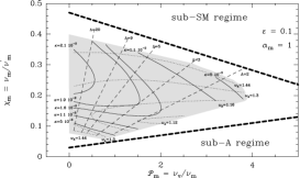
5.2.2 Parameter space of cold, adiabatic MAES

The parameter space of cold MAES is obtained by varying the set of free disc parameters ($\varepsilon,\alpha_{m},{\cal P}_{m},\chi_{m}$). We choose to fix the values of both $\varepsilon$ and $\alpha_{m}$ and represent the parameter space with the remaining parameters (Fig. 4). Numerical solutions are only found inside the shaded areas, where we also plot levels of two jet parameters $\omega_{A}$ and $\kappa$. This region is embedded inside a larger region (thick dashed lines), obtained by two analytical constraints. The first one arises from the requirement that jets become super-SM and is thus related to the disc vertical equilibrium. The second emerges from the requirement that jets must become super-Alfvénic, namely $\omega_{A}>1$, providing the lower limits in the same plots. These two analytical constraints strongly depend on both $\alpha_{m}$ and $\varepsilon$. Cold, adiabatic MAES have the following properties:

$\bullet$ The parameter space is very narrow, with typical values $\xi\sim 10^{-2}$ and $\mu\sim 1$. No solution has been found outside the range $0.001<\varepsilon<0.3$ and $0.3\leq\alpha_{m}<3$. The corresponding jet parameters lie in the range $10<\lambda<100$ and $0.001<\kappa<0.03$.

$\bullet$ The parameter space shrinks considerably with $\alpha_{m}$, because of the extreme sensibility of $B_{\phi}^{+}$ to it (Casse & Ferreira 2000a). Note however that $\alpha_{v}=\alpha_{m}\mu^{1/2}{\cal P}_{m}$ is usually smaller than $\alpha_{m}$.

$\bullet$ No solution has been found with a dominant viscous torque ($\Lambda\ll 1$): the reason lies in the imposed geometry of the Alfvén surface (conical). On the other hand, high-$\omega_{A}$ solutions (those with large jet radius) exist only for magnetically-dominated discs ($\Lambda\gg 1$).

$\bullet$ The required turbulence anisotropy increases with both $\Lambda$ and $\alpha_{m}$, following the scaling $\chi_{m}\sim\Lambda\varepsilon\alpha_{v}\alpha_{m}$ provided by Eq. (65).

5.3 “Warm” configurations

5.3.1 Entropy generation inside the disc

As seen in Sect. 2.3.2, the disc energy equation (33) is such a mess that all works on accretion discs used simpified assumptions. In fact using an isothermal or adiabatic prescription for the temperature vertical profile may be an over simplification, that may have led to such a small parameter space. One way to tackle the energy equation is to solve

$$\rho T\frac{DS}{Dt}=\rho T\vec{u}_{p}\cdot\nabla S=Q$$ (79)

where the entropy source $Q=\Gamma-\Lambda$ is prescribed and describes the local net effect of all possible heating $\Gamma$ and cooling $\Lambda$ terms. The sources of heating are:

$\hookrightarrow$ $\Gamma_{eff}=\eta_{m}J^{2}_{\phi}\ +\ \eta^{\prime}_{m}J^{2}_{p}\ +\ \eta_{v}\left|r\nabla\Omega\right|^{2}$ the effective Joule and viscous dissipations;

$\hookrightarrow$ $\Gamma_{turb}$ due to turbulent energy deposition, not described by anomalous coefficients;

$\hookrightarrow$ $\Gamma_{ext}$ some external source of energy (like protostellar UV or X-rays, or cosmic rays).

On the other hand, the cooling sources are

$\hookrightarrow$ $\Lambda_{rad}=\nabla\cdot\vec{S}_{rad}$ radiative losses in optically thick or thin media;

$\hookrightarrow$ $\Lambda_{turb}$ turbulent transport that may be described by kinetic theory or due to large scale motions like convection (in Eq. (33) $\nabla\cdot\vec{q}_{turb}=\Lambda_{turb}-\Gamma_{turb}$).

In our simplified approach, we prescribe both the shape and amplitude of $Q$, but consistently with energy conservation. We make therefore two assumptions: (1) there is no net input of turbulent energy in the volume ${\cal V}$ occupied by the MAES, namely $P_{turb}=\int_{\cal V}\left(\Gamma-\Lambda\right)_{turb}d^{3}{\cal V}=0$ and (2) the power deposited by any external medium is negligible, ie. $P_{ext}=\int_{\cal V}\Gamma_{ext}d^{3}{\cal V}=0$. With these assumptions, the only remaining source of energy is accretion of the laminar flow: turbulence can only redistribute energy from one place to another one.

Accretion is possible because of the torque due to the mean magnetic field (jet) and the turbulent (“viscous”) torque. Accretion energy released by the first torque is converted into a MHD Poynting flux leaving the disc (and feeding the jets) and heat through local Joule dissipation. Accretion energy released by the “viscous” torque is conventionaly thought as being converted into heat through dissipation. But note that if such a torque arises from field lines connecting two disc radii, one would then expect also an outward flux of energy, which would be dissipated above the disc surface (Heyvaerts & Priest 1989, Miller & Stone 2000, Machida et al. 2000). Anyway, these two heating sources ($\Gamma_{eff}$) build up a local gas thermal energy reservoir which decreases because of the local cooling terms. Thus, the total power related to dissipation inside the disc (ie. not directly put into the jets) is $P_{diss}=\int_{\cal V}\Gamma_{eff}d^{3}{\cal V}$. In a conventional picture of accretion discs, such a power is finally radiated away, either at the disc surfaces only, or also in some chromosphere. Here, we assume that a fraction $f$ of this power is in fact not lost by the plasma but provides an extra source of entropy $Q$, namely

$$f=\frac{\int_{\cal V}Qd^{3}{\cal V}}{\int_{\cal V}\Gamma_{eff}d^{3}{\cal V}}$$ (80)

This expression is consistent with global energy conservation, the parameter $f$ being free and varying from $0$ (“cold” MAES) to 1 (“warm” or magneto-thermally driven jets). A value of $f$ larger than unity would require an extra source of energy. We need now to specify the vertical (self-similar) profile of $Q$. Obviously, this introduces so many degrees of freedom that we do not dare anymore to look for the parameter space. Instead, we will look for extreme configurations and try to derive quantitative results.

Figure 5: Left: Variation of jet parameters with $f$. As $f$ increases, jets get hotter, denser and with a smaller magnetic lever arm $\lambda$. After some threshold, depending on the other MAES (turbulence) parameters, thermal effects become so important that super-A jets can be obtained with slow-rotators ($\omega_{A}<1$). Right: Two new extreme MAES with an additional heating Q. If Q is very large at the disc surface ($f\sim 1$), hot and dense jets are produced (solid curves) whereas cold and very tenuous jets (dashed curves) are obtained if Q is almost inexistent ($f=5\ 10^{-5}$). Lower pannels show the effective turbulent heating $\Gamma_{eff}$ and the prescribed entropy source $Q$ at a radius $r_{o}$, normalized to the same quantity.

5.3.2 Dynamical effects

The steady-state energy equation (79) can be explicitely written

$$Q=\rho T\frac{DS}{Dt}=\rho\frac{DH}{Dt}-\frac{DP}{Dt}=\frac{\gamma}{\gamma-1}\frac{k_{B}}{m_{p}}\rho\vec{u}_{p}\cdot\nabla T-\vec{u}_{p}\cdot\nabla P\ .$$ (81)

We then see that the main influence of a non-zero $Q$ is on the temperature and pressure vertical gradients (thin disc), thus at the disc surface. But this is precisely the place where such gradients are required for ejection (Sect. 4.1.3)! Therefore, allowing some energy deposition at the disc surface has two major effects:

• (1) The initial jet temperature ($T^{+}$) is increased and may thereby provide a non-negligible initial enthalpy $H$ (“warm” jets). Indeed, the Bernoulli integral becomes

  $$E(a)=\frac{u^{2}}{2}\ +\ H\ +\ \Phi_{G}\ -\ \Omega_{*}\frac{rB_{\phi}}{\eta}\ -\ \int^{s}_{s^{+}}\frac{Q(s^{\prime},a)}{\rho(s^{\prime},a)u_{p}(s^{\prime},a)}ds^{\prime}$$ (82)

  where $s$ is a curvilinear coordinate along the magnetic surface and $s^{+}$ represents the disc surface. If $Q$ remains positive above $s^{+}$, it offers an additional energy reservoir for plasma. Moreover, the total energy feeding a magnetic surface,

  $$E(a)=\frac{\Omega_{o}^{2}r_{o}^{2}}{2}\left(2\lambda-3+\frac{2\gamma}{\gamma-1}\frac{T^{+}}{T_{o}}\varepsilon^{2}\right)\ .$$ (83)

  is affected by the heating that already occurred in the underlying layers. Such an heating may provide a ratio $T^{+}/T_{o}$ larger than unity, possibly allowing to relax the constraint on minimum field lines inclination.

• (2) If $Q$ is relevant in the upper resistive layers, then it will increase also the plasma pressure gradient. This will enhance the ejected mass flux (and lower the magnetic lever arm) and might therefore have tremendous consequences on jet dynamics.

We used only one type of vertical profile $f_{Q}(s)$, changing the value of the parameter $f$. The chosen profile provides $Q\simeq 0$ inside the disc ($x<0.5$), an increase until a maximum value (fixed by $f$) around $x\leq 1$, then a decrease to zero (adiabatic behaviour) after roughly one scale height (see Casse & Ferreira 2000b). As $f$ increases (all other MAES parameters being held constant), one goes from cold ($T^{+}<T_{o}$), tenuous ($\kappa<0.02$) jets from fast rotators ($\omega_{A}>1$) to hot ($T^{+}\gg T_{o}$), dense ($\kappa>0.1$) jets from slow rotators ($\omega_{A}<1$). Namely, the presence of some chromospheric heating allows a smooth transition from “cold” (purely magnetically-driven) to “warm” (magneto-thermaly driven) jets.

Another class of “cold” solutions can also be designed. Indeed, if local cooling is not sufficient inside the disc ($Q>0$ for $x<1$), the plasma pressure increases which provides the disc a stronger support against both tidal and magnetic compression. As a result, the magnetic field lines can be more bent than in the previous adiabatic or isothermal solutions. Such a large curvature hinders mass to be ejected ($\kappa$ may be as small as $10^{-4}$ and $\lambda\sim 400$) but a vertical equilibrium can nevertheless be reached. Thus, entropy generation inside the disc removes the limits found on the “cold” parameter space described earlier.

5.3.3 Global energy conservation

We suppose that a MAES is settled around a central object of mass $M$, between an inner radius $r_{i}$ and some outer radius $r_{e}$. At this outer radius, the structure is fed with an accretion rate $\dot{M}_{ae}=\dot{M}_{a}(r_{e})$. Mass conservation then writes $\dot{M}_{ae}-2\dot{M}_{j}=\dot{M}_{ai}$ and the fraction of ejected mass is

$$\frac{2\dot{M}_{j}}{\dot{M}_{ae}}=1-\left(\frac{r_{i}}{r_{e}}\right)^{\xi}\simeq\xi\ln\frac{r_{e}}{r_{i}}$$ (84)

the last expression being valid only for a very small ejection efficiency $\xi\ll 1$. The local energy conservation equation is

$$\nabla\cdot\left[\rho\vec{u}_{p}\left(\frac{u^{2}}{2}\ +\ \Phi_{G}\ +\ H\right)\ +\ \vec{S}_{MHD}\ -\ \vec{u}\cdot{\mathsf{T}}\right]=\rho T\vec{u}_{p}\cdot\nabla S\ -\ \Gamma_{eff}$$ (85)

whereas the second law of thermodynamics (79) provides

$$Q=\rho T\vec{u}_{p}\cdot\nabla S=\Gamma_{eff}\ +\ (\Gamma_{turb}\ -\ \Lambda_{turb})\ +\ \Gamma_{ext}\ -\ \nabla\cdot\vec{S}_{rad}$$ (86)

Figure 6: Sketch of the volume used for the calculation of the global energy conservation.

To get the global energy conservation, we integrate this equation on the volume ${\cal V}$ occupied by the disc. We thus define $\Sigma^{+}$ and $\Sigma^{-}$ as the disc surfaces and $\Sigma_{i}$ ($\Sigma_{e}$) the lateral surfaces at $r=r_{i}$ ($r=r_{e}$, see Fig. (6)). After integration, we get

$$P_{acc}+P_{ext}+P_{turb}=2P_{jet}+2P_{rad}$$ (87)

where the accretion power $P_{acc}$, ie. the power released by the accretion flow, is the difference between what comes in at $r_{e}$ and goes out at $r_{i}$. As said previously, we assumed $P_{ext}=P_{turb}=0$ (neither an external source of energy, nor a significant input of turbulent energy). Thus, all available power $P_{acc}$ is shared between radiative losses at the disc surfaces $P_{rad}=\int_{\Sigma^{\pm}}\vec{S}_{rad}\cdot\vec{dS}$ and jet power $P_{jet}=\int_{\Sigma^{\pm}}\rho\vec{u_{p}}E(a)\cdot\vec{dS}$. It is usefull to introduce the fiducial quantity

$$P_{lib}\equiv\eta_{lib}\frac{GM\dot{M}_{ae}}{2r_{i}}\simeq 2.5\,10^{32}\ \left(\frac{M}{M_{\odot}}\right)\left(\frac{\dot{M}_{ae}}{10^{-7}M_{\odot}/yr}\right)\left(\frac{r_{i}}{0.1\mbox{ AU}}\right)^{-1}\ \mbox{erg s}^{-1}$$ (88)

where $\eta_{lib}$ is a term roughly equal to unity. Within our self-similar framework, energy conservation of a thin (or slim) disc writes

$$\frac{P_{acc}}{P_{lib}} = (1-\xi)\left(1+\frac{1}{2}\frac{\varepsilon\Lambda}{1+\Lambda}\right)$$ (89)

$$\frac{2P_{jet}}{P_{lib}} = \frac{\Lambda}{1+\Lambda}\left|\frac{B^{+}_{\phi}}{qB_{o}}\right|\ +\ \frac{2\gamma}{\gamma-1}\frac{T^{+}}{T_{o}}\xi\varepsilon^{2}\ -\ \xi$$ (90)

$$\frac{2P_{rad}}{P_{lib}} = (1-f)\frac{P_{diss}}{P_{lib}}=\frac{P_{acc}-2P_{jet}}{P_{lib}}$$ (91)

See Casse & Ferreira (2000b) for the derivation of these expressions. Three important remarks. First, the absolute limit for the ejection efficiency is $\xi=1$; Second, the real energy release is $P_{acc}$, comparable to $P_{lib}$ only for low ejection indices. Finally, the MHD Poynting flux feeding the jets depends directly on the amount of toroidal field at the disc surface. Thus, magnetically-dominated discs ($\Lambda\gg 1$) may still produce some disc luminosity, provided $|B^{+}_{\phi}|<qB_{o}$ (and $f<1$). For $f\sim 0$ we found solutions with a ratio $P_{jet}/P_{rad}$ varying between 0.1 and 10.

5.3.4 Preliminary conclusions

From this study, we are forced to conclude that thermal effects have an outrageous quantitative importance on jet launching. In a way, this is fortunate since we can now recover and understand the parameter space obtained with numerical MHD simulations. Although “cold”, the simulated jets have enormous mass loads and correspondingly small magnetic lever arms ((eg. $\kappa\sim 0.6$, $\lambda\sim 3.5$, Ouyed & Pudritz 1999). This may be easily achieved from an accretion disc where a significant entropy generation took place at the disc surface ($f>0.1$), followed right afterwards by a strong cooling ($Q<0$ for $x>1$). In this way, very dense but cold (well, after some time) jets can indeed be produced. Remember that the bottom of the computational box has nothing to do with the real disc surface.

A major drawback of such a conclusion is that any quantitative prediction (eg. the value of $\xi$) requires to treat the energy equation. We must therefore inject our knowledge on MHD turbulence and its (possibly non local) energy transport properties ! Besides, illumination effects by the central protostar may also be important (since it heats up the disc surface).

5.4 Observational predictions

5.4.1 Accretion discs

Whether or not the disc remains geometrically thin depends on its internal temperature, hence on the energy equation. Although the energy transport processes are unknown, an opaque disc must radiate at its surfaces all deposited energy. This translates into an effective temperature at the photosphere $z=h_{phot}(r)$

$$\sigma T_{eff}^{4}=\int_{0}^{h_{phot}}\nabla\cdot\vec{S}_{rad}\,dz=(1-f)\int_{0}^{h_{phot}}\left[\eta_{m}J^{2}_{\phi}\ +\ \eta^{\prime}_{m}J^{2}_{p}\ +\ \eta_{v}\left|r\nabla\Omega\right|^{2}\right]\,dz$$ (92)

The rhs of this equation can be estimated whereas the effective and central temperatures are crudely related through $T_{eff}\sim T_{o}\tau^{-1/4}$, where $\tau\sim\kappa\rho_{o}h_{phot}$ is the disc optical depth. Now, assuming that $h_{phot}(r)\sim h(r)$ and choosing the dominant disc opacity to be the grain opacity $\kappa=0.1\ T^{1/2}\ \mbox{cm}^{2}\mbox{g}^{-1}$ (Bell & Lin 1994), allow us to estimate both the local disc aspect ratio $\varepsilon$ and optical depth $\tau$ without even solving the energy equation. Once we have $\varepsilon=h/r$, we can express all disc quantities in terms of the remaining free parameters. Hence, steady-state theory of MAES requires the following physical conditions in a disc settled around a low-mass protostar:

$$\frac{h}{r} = 5\ 10^{-2}\ \alpha_{v}^{-1/9}(1-f)^{1/9}\left(\frac{M}{M_{\odot}}\right)^{-1/3}\left(\frac{\dot{M}_{eff}}{10^{-7}M_{\odot}/yr}\right)^{2/9}$$

$$\tau \simeq 7.5\ \alpha_{v}^{-8/9}(1-f)^{-1/9}\left(\frac{M}{M_{\odot}}\right)^{1/3}\left(\frac{\dot{M}_{eff}}{10^{-7}M_{\odot}/yr}\right)^{7/9}\left(\frac{r_{o}}{1\ \mbox{AU}}\right)^{-1}$$

$$T_{eff} = 168\ (1-f)^{1/4}\left(\frac{M}{M_{\odot}}\right)^{1/4}\left(\frac{\dot{M}_{eff}}{10^{-7}M_{\odot}/yr}\right)^{1/4}\left(\frac{r_{o}}{1\ \mbox{AU}}\right)^{-3/4}\mbox{ K}$$

$$T_{o} = 276\ \alpha_{v}^{-2/9}(1-f)^{2/9}\left(\frac{M}{M_{\odot}}\right)^{1/3}\left(\frac{\dot{M}_{eff}}{10^{-7}M_{\odot}/yr}\right)^{4/9}\left(\frac{r_{o}}{1\ \mbox{AU}}\right)^{-1}\mbox{ K}$$

$$\Sigma_{o}=2\rho_{o}h = 9\ \alpha_{v}^{-7/9}(1-f)^{-2/9}\left(\frac{M}{M_{\odot}}\right)^{1/6}\left(\frac{\dot{M}_{eff}}{10^{-7}M_{\odot}/yr}\right)^{5/9}\left(\frac{r_{o}}{1\ \mbox{AU}}\right)^{-1/2}\mbox{ g.cm}^{-2}$$

$$B_{o} = 1.3\ \mu^{1/2}\alpha_{v}^{-4/9}(1-f)^{-1/18}\left(\frac{M}{M_{\odot}}\right)^{5/12}\left(\frac{\dot{M}_{eff}}{10^{-7}M_{\odot}/yr}\right)^{7/18}\left(\frac{r_{o}}{1\ \mbox{AU}}\right)^{-5/4}\mbox{ G}$$

$$\frac{u_{o}}{\Omega_{K}r_{o}} = 3\ 10^{-3}\ \alpha_{v}^{7/9}(1-f)^{2/9}(1+\Lambda)^{5/9}\left(\frac{M}{M_{\odot}}\right)^{-2/3}\left(\frac{\dot{M}_{a}(r_{o})}{10^{-7}M_{\odot}/yr}\right)^{4/9}$$

where $\dot{M}_{eff}=\dot{M}_{a}(r_{o})/(1+\Lambda)$. Parameters $\mu\sim 1$ and $\xi$ are provided by the MHD solution. Note that the self-similar scaling $h(r)\propto r$ is here slightly violated since $\dot{M}_{a}\propto r_{o}^{\xi}$. But such a deviation remains minor for $\xi<0.1$. Care must be taken when looking at those expressions because $\Lambda$ is imposed by Eq. (65) and depends thus on ($\varepsilon,\alpha_{m},{\cal P}_{m},\chi_{m}$). But this choice allows to recover both radial scalings and values of a standard accretion disc when $\xi=f=\Lambda=0$. To get a super-A solution with $\alpha_{v}=\alpha_{m}{\cal P}_{m}\mu^{1/2}\ll 1$ one probably needs to play around with $f$ (for $f=0$ the parameter space is already known and requires large values of $\alpha_{v}$).

Several observational diagnostics could reveal the presence of a magnetized disc driving jets: (i) the measure of a large (organized) disc magnetic field; (ii) optically thin regions or some lack of disc emission (for models with $\Lambda\gg 1$); (iii) a different spectral energy distribution (the effective temperature scales as $r_{o}^{(\xi-3)/4}$) for discs with a large ejection index $\xi$. But usually, SED are tricky to interpret and we don’t have the resolution yet to measure disc magnetic fields.

5.4.2 Self-collimated jets

The most acurate tool to discriminate between models is to confront theoretical predictions with recent spatially resolved observations of the inner wind structure of TTS in forbidden emission lines of [O i], [S ii] and [N ii]. Indeed, being optically thin, these lines carry information on both dynamic and thermodynamic properties of the whole volume of emission. So, one way to use this information is to construct the following synthetic observations and comparing them to real ones:

• Emission maps, which must then be convolved to typical resolutions in order to predict what would be the observed jet morphology and collimation properties (eg. displacement of emission peaks, jet FWHM as a function of distance).

• Line profiles, like those obtained using long-slit spectroscopy, and integrated profiles.

• Integrated line fluxes as well as their correlations with the disc accretion rate.

• Forbidden line ratios, which reflect the values of the electron density, ionisation fraction and local temperature.

While the first two observations offer constraints on the jet dynamics, the last ones test mainly the heating and ionization mechanisms along the jet. We already have a dynamical model providing us with jet density and velocity. The gas emissivity then requires to know the jet thermal and ionization states. With that in hand, we can easily compute synthetic observations and compare them to real ones. This has first been done by Safier (1993) using Blandford & Payne jet solutions. We can now do the same with models of MAES that take self-consistently into account the disc-jet interrelations.

Cabrit et al. (1999), using parameterized temperature and ionization fraction, produced synthetic maps and long-slit spectra that were nicely compatible with observations (Shang et al. (1998) did the same for X-winds). But more reliable predictions require actually solving for the jet thermal and ionization state, given some local heating mechanism. Our models being stationary, we cannot invoke shocks as being the heating process. Moreover, this would require the introduction of additional free parameters ! This is even worse if we rely on some small scale turbulence, providing a means to dissipate locally jet kinetic energy. The only self-consistent mechanism, intrinsic to MHD flows of low ionization, is ambipolar diffusion (see Sect. 2.2.3).

Using this (unavoidable) effect to heat up jets, Garcia et al. (2001) solved the energy equation along the jet as well as its ionization state, taking into account several heavy elements (C, N, O, S, Ca, Mg, Fe…), photoionization heating and cooling by Hydrogen recombination lines. They used cold (isothermal) MAES solutions obtained by Ferreira (1997) with $\xi\sim 0.01$. Jet widths and variations in line profiles with distance and line tracer are well reproduced. However, predicted maximum velocities are too high, total densities too low and, as a result, the low-velocity [O i] component is too weak. Thus, denser and slower MHD jets are required.

In the solutions used, ejected plasma reaches its asymptotic speed $u_{\infty}\simeq\Omega_{o}r_{o}\sqrt{2\lambda-3}$, which is typically 10 times the Keplerian speed at the field line footpoint. Even though there is some inclination effect that decreases the observed jet velocity, it is still too large: emission from the jet inner region is important. Thus, one needs to decrease the jet terminal speed, which requires to diminish the magnetic lever arm $\lambda$, ie. to increase the ejection index $\xi$ (which automatically provides a denser jet). However, models with values of $\xi$ larger than 0.01 require an additional heating at the disc surface. How much exactly remains to be worked out.

6 Some perspectives

At this stage, one can have confidence in several things: (1) we know exactly, in a model independent way, how accretion discs can steadily drive jets; (2) jet properties (velocity, collimation) are strongly dependent on the mass flux allowed by the disc; (3) such a mass flux is highly sensitive to the critical disc energy equation; (4) we don’t know if real accretion discs ever meet the required physical conditions for MAES.

The MAES paradigm is based on the belief that a large scale magnetic field is threading the disc on a large radial extension. This ensures some kind of cylindrical geometry (actually a conical Alfvén surface), whereas ejection from a small disc region, as in X-winds (Shu et al. 1994), would provide a spherical expansion of the field lines (and a more or less spherical Alfvén surface). Such a basic fact provides very different jet behaviours (see appendix B in Casse & Ferreira 2000a), but the underlying accretion/ejection mechanism remains exactly the same. As we saw, comparing synthetic to real observations is quite a powerful tool to eliminate MAES models and will probably help to discriminate between “disc winds” and “X-winds”. We know now that, inside the MAES paradigm, YSOs require active chromospheres and coronae. Such a work must therefore be continued, in the hope that a characterization of their properties can indeed be achieved. In parallel, a thorough theoretical (analytical and numerical) work must be performed to understand how instabilities in magnetized discs may lead to turbulence and anomalous transport.

What is not addressed by current models of MAES, is the interaction with the central object. However, including such an interaction and even allowing for some energetic events to occur there (eg. such as unsteady mass ejection) would not perturb the above picture. The main strength of the simplified version studied here (pure “disc winds”) is to provide clear answers to the basic phenomena of correlated accretion and ejection. Anyway, such an interaction is unavoidable and, for a young protostar, may be the ingredient solving the “angular momentum problem”. This problem arises from the idea that a protostar of masse $M$ and radius $R$ arises from the collapse of a rotating molecular cloud. The specific angular momentum of these clouds is typically $10^{21}\mbox{ cm}^{2}$/s (Goodman et al. 1993). A typical T-Tauri star (optically revealed protostar) rotates with a period of 8 days, which provides a specific angular momentum of the order of some $10^{17}\mbox{ cm}^{2}$/s. Where has all this angular momentum gone ? Evidently, we can assume that a (magnetic) braking occurred during the collapse, but no model provided yet a good account of the angular momentum transport. A conservative approach is to assume that, once formed, the protostar is rotating close to break-up, with a period $P=2\pi\sqrt{R^{3}/GM}$ ($\sim$ 1 day). But the corresponding specific angular momentum is still an order of magnitude larger than that of a T-Tauri star. Thus, another very efficient braking must occur during the embedded phase. Moreover, there are some observational evidences that accretion discs play a role in braking down T-Tauri stars. Indeed, even though they are contracting and accreting material, T-Tauri stars seem to maintain a constant angular velocity (Bouvier et al. 1997). The idea is therefore to imagine an interaction with the accretion disc providing a negative torque on the protostar.

If nothing prevents the accreting disc material to approach the stellar surface, an equatorial boundary layer will form at the interface (eg. Popham et al. 1993). But because matter is rotating faster than the protostar, such an interaction can only lead to a spin-up of the protostar. The current paradigm is a magnetospheric interaction with the disc. The protostar is believed to have a large scale magnetic field able to truncate the disc by forcing the accreting material to leave the equatorial plane and follow the magnetosphere. A spin-down is then obtained whenever the field is large enough so that the truncation radius (magnetopause) is located beyond the co-rotation radius $r_{co}$, defined by $\Omega_{star}=\Omega_{disc}(r_{co})$. In this case, the protostellar angular momentum is deposited into the inner disc region… which then must expell it !

Some models rely on a very efficient disc turbulent viscosity that would radially transport both disc and protostellar angular momentum (eg. Li 1996). Or, if not throughout all the disc, just on a small region until it reaches a region located beyond the closed magnetosphere. There, open field lines could transport this excess of angular momentum in a jet (“X-winds” by Shu et al. 1994). As said previously, these X-winds carry away the exact angular momentum at a rate allowing accretion: they are therefore disc-winds, but produced from a tiny disc region (see also Fendt & Elstner 2000). It may be more economic to use the protostellar angular momentum and rotational energy to directly produce another jet component. This can be done whenever the protostellar magnetic moment has the same polarity as the disc magnetic field. A magnetic neutral line forms at the equatorial plane, where reconnection of the two fields takes place. Above this reconnection site, a fraction of the accreting matter can be loaded onto newly opened protostellar field lines (Ferreira et al. 2000). Such Reconnection X-winds arise from a different ejection mechanism: they expell disc material thanks to the protostellar rotational energy. This is the reason why they can brake down very efficiently the protostar, on time scales compatible with observations.

It took almost 30 years to prove that accretion discs can indeed launch jets that carry away a sizeable fraction of their angular momentum. Investigations of the magnetospheric interaction between a protostar and its circumstellar disc are just beginning and the situation is far more complex than for discs. Lots of analytical efforts have still to be done, probably guided by the insights provided by numerical simulations.

References

Balbus A.S., Hawley J.F. 1991, ApJ 376, 214
A powerful local shear instability in weakly magnetized disks.I- Linear analysis

Bell K.R., Lin D.N.C. 1994, ApJ 427, 987
Using FU Orionis outbursts to constrain self-regulated protostellar disk models

Blandford R.D., Rees M.J. 1974, MNRAS 169, 395
A “twin-exhaust” model for double radio sources

Blandford R.D. 1976, MNRAS 176, 465
Accretion disc electrodynamics- A model for double radio sources

Blandford R.D., Payne D.G. 1982, MNRAS 199, 883
Hydromagnetic flows from accretion discs and the production of radio jets

Bouvier J., Forestini M., Allain S. 1997, A&A 326, 1023
The angular momentum evolution of low-mass stars.

Brandenburg A., Donner K.J. 1997, MNRAS 288, L29
The dependence of the dynamo alpha on vorticity

Breitmoser E., Camenzind M. 2000, A&A 361, 207
Collimated outflows of rapidly rotating young stellar objects. Wind equation, GSS equation and collimation

Bridle H.A., Perley A.R. 1984 ARA&A 22, 319
Extragalactic radio jets

Cabrit S., Ferreira J., Raga A.C. 1999, A&A 343, L61
Forbidden lines from T Tauri disk winds. I. High magnetic torque models

Camenzind M. 1990, in G. Klare (ed.), Rev. in Modern Astrophysics, 3, Springer-Verlag, Berlin
Magnetized Disk-Winds and the Origin of Bipolar Outflows.

Cantó J. 1980, A&A 86, 327
A stellar wind model for Herbig-Haro objects

Cao X., Jiang D.R. 1999, MNRAS 307, 802
Correlation between radio and broad-line emission in radio-loud quasars

Casse F., Ferreira J. 2000a, A&A 353, 1115
Magnetized accretion-ejection structures. IV. Magnetically-driven jets from resistive, viscous, Keplerian discs

Casse F., Ferreira J. 2000b, A&A 361, 1178
Magnetized accretion-ejection structures. V. Effects of entropy generation inside the disc

Chan K.L., Henriksen R.N. 1980, ApJ 241, 534
On the supersonic dynamics of magnetized jets of thermal gas in radio galaxies

Ciolek G.E., Mouschovias, T. 1995, ApJ 454, 194
Ambipolar Diffusion, Interstellar Dust, and the Formation of Cloud Cores and Protostars. IV. Effect of Ultraviolet Ionization and Magnetically Controlled Infall Rate

Contopoulos J., Lovelace R.V.E. 1994, ApJ 429, 139
Magnetically driven jets and winds: Exact solutions

Contopoulos J., Sauty C. 2001, A&A 365, 165
The origin of molecular protostellar outflows

Crutcher R.M. 1999, ApJ 520, 706
Magnetic Fields in Molecular Clouds: Observations Confront Theory

DeCampli W.M. 1981, ApJ 244, 124
T Tauri winds

Fendt C., Camenzind M., Appl S. 1995, A&A 300, 791
On the collimation of stellar magnetospheres to jets. I. Relativistic force-free 2D equilibrium.

Fendt C., Elstner D. 2000, A&A 363, 208
Long-term evolution of a dipole type magnetosphere interacting with an accretion disk. II. Transition into a quasi-stationary spherically radial outflow

Ferreira J., Pelletier G. 1993, A&A 276, 625
Magnetized accretion-ejection structures. I. General statements

Ferreira J., Pelletier G. 1995, A&A 295, 807
Magnetized accretion-ejection structures. III. Stellar and extragalactic jets as weakly dissipative disk outflows.

Ferreira J. 1997, A&A 319, 340
Magnetically-driven jets from Keplerian accretion discs

Ferreira J., Pelletier G., Appl S. 2000, MNRAS 312, 387
Reconnection X-winds: spin-down of low-mass protostars

Garcia P., Ferreira J., Cabrit S., Binette L., Raga A., Dougados C., Casse F., Lavalley C. 2001 in “Emission Lines from Jet Flows” Isla Mujeres (Mexico)
Forbidden line emission from MHD disk winds and time-variable jets: comparison with T Tauri microjets

Gomez de Castro A.I., Pudritz R.E. 1993, ApJ 409, 748
The origin of forbidden line emission from young stellar objects

Goodman A.A., Benson P.J., Fuller G.A., Myers P.C. 1993, ApJ 406, 528
Dense cores in dark clouds. VIII - Velocity gradients

Hartmann L., McGregor K.B. 1982, ApJ 259, 180
Protostellar mass and angular momentum loss

Heyvaerts J., Norman C.A. 1989, ApJ 347, 1055
The collimation of magnetized winds

Heyvaerts J., Priest E.R. 1989, A&A 216, 230
A model for a non-Keplerian magnetic accretion disk with a magnetically heated corona

Heyvaerts J., Priest E.R., Bardou A. 1996, ApJ 473, 403
Magnetic Field Diffusion in Self-consistently Turbulent Accretion Disks

Jones D.L., Werhle A.E., Meier D.L., Piner B.G. 2000, ApJ 534, 165
The radio jets and accretion disk in NGC 4261

Königl A. 1982, ApJ 261, 115
On the nature of bipolar sources in dense molecular clouds

Königl A. 1986, Can. J. Phys. 64, 362
Stellar and galactic jets: theoretical issues

Krasnopolsky R., Li Z.-Y., Blandford R. 1999, ApJ 526, 631
Magnetocentrifugal Launching of Jets from Accretion Disks.I- Cold Axisymmetric Flows

Kudoh T., Matsumoto R., Shibata K. 1998, ApJ 508, 186
Magnetically Driven Jets from Accretion Disks. III. 2.5-dimensional Nonsteady Simulations for Thick Disk Case

Kwan J. 1997, ApJ 489, 284
Warm Disk Coronae in Classical T Tauri Stars

Lery T., Henriksen R.N., Fiege J.D. 1999, A&A 350, 254
Magnetised protostellar bipolar outflows. I. Self-similar model with Poynting flux

Lery T., Heyvaerts J., Appl S., Norman C.A. 1999, A&A 347, 1055
Outflows from magnetic rotators. II. Asymptotic structure and collimation

Li J. 1996, ApJ 456, 696
Magnetic Interaction between Classic T Tauri Stars and Their Associated Disks

Li Z.-Y. 1995, ApJ, 444, 848
Magnetohydrodynamic disk-wind connection: Self-similar solutions

Li Z.-Y. 1996, ApJ 465, 855
Magnetohydrodynamic disk-wind connection: Magnetocentrifugal winds from ambipolar diffusion-dominated accretion disks

Livio M. 1997, in IAU 163, Accretion Phenomena and Related Outflows, ASP Conf Series 121
The Formation Of Astrophysical Jets

Lovelace R.V.E. 1976, Nature 262, 649
Dynamo model of double radio sources

Lovelace R.V.E., Wang J.C.L., Sulkanen M.E. 1987, ApJ 62, 1
Self-collimated electromagnetic jets from magnetized accretion disks

Lovelace R.V.E., Romanova M.M., Bisnovatyi-Kogan G.S. 1999, ApJ 514, 368
Magnetic Propeller Outflows

Machida M., Hayashi M.R., Matsumoto R. 2000, ApJ, 532, L67
Global Simulations of Differentially Rotating Magnetized Disks: Formation of Low-$\beta$; Filaments and Structured Coronae

Mestel L. 1968, MNRAS 138, 359
Magnetic braking by a stellar wind-I

Miller K.A., Stone J.M. 2000, ApJ 584, 398
The Formation and Structure of a Strongly Magnetized Corona above a Weakly Magnetized Accretion Disk

Mirabel I.F.,Rodriguez L.F. 1999, ARA&A 37, 409
Sources of Relativistic Jets in the Galaxy

Okamoto I. 1999, MNRAS 307, 253
Do magnetized winds self-collimate?

Ostriker E. 1997, ApJ 486, 291
Self-similar Magnetocentrifugal Disk Winds with Cylindrical Asymptotics

Ouyed R., Pudritz, R.E. 1999, MNRAS 309, 233
Numerical simulations of astrophysical jets from Keplerian discs -III. The effects of mass loading

Ouyed R., Pudritz, R.E. 1997, ApJ 484, 794
Numerical Simulations of Astrophysical Jets from Keplerian Disks -II. Episodic Outflows

Parker E.N. 1958, ApJ 128, 664
Dynamics of the interplanetary gas and magnetic fields

Pelletier G., Pudritz R.E 1992, ApJ 394, 117
Hydromagnetic disk winds in young stellar objects and active galactic nuclei

Popham R., Narayan R., Hartmann L., Kenyon S. 1993, ApJ 415, L127
Boundary Layers in Pre-Main-Sequence Accretion Disks

Pudritz, R.E., Norman C.A. 1983, ApJ 274, 677
Centrifugally driven winds from contracting molecular disks

Ray T.P., Mundt R., Dyson J.E., Falle S., Raga A.C. 1996, ApJ 468, L103
HST Observations of Jets from Young Stars

Rekowski M.v., Rüdiger G., Elstner D. 2000, A&A 353, 813
Structure and magnetic configurations of accretion disk-dynamo models

Rosso F., Pelletier G. 1994, A&A 287, 325
A variational method for solving fast MHD flows. Consequences for stellar and extragalactic jets

Safier P.N. 1993, ApJ 408, 115
Centrifugally driven winds from protostellar disks. I - Wind model and thermal structure

Sauty C., Tsinganos K., Trussoni E. 1999, A&A 348, 327
Nonradial and nonpolytropic astrophysical outflows. IV. Magnetic or thermal collimation of winds into jets?

Sergeant S., Rawlings S., Maddox S.J., Baker J.C., Clements D., Lacy M., Lilje P.B. 1998, MNRAS 294, 494
The radio-optical correlation in stepp spectrum quasars

Shakura N.I., Sunyaev R.A. 1973, A&A 24, 337
Black holes in binary systems. Observational appearance

Shakura N.I., Sunyaev R.A., Zilitinkevich S.S. 1978, A&A 62, 179
On the turbulent energy transport in accretion discs

Shang H., Shu F.H., Glassgold A.E. 1998, ApJ 493, L91
Synthetic Images and Long-slit Spectra of Protostellar Jets

Shibata K., Uchida Y. 1985, PASJ, 37, 31
A magnetodynamic mechanism for the formation of astrophysical jets. I - Dynamical effects of the relaxation of nonlinear magnetic twists

Shu F.H., Najita J., Ostriker E., Wilkin F., Ruden S., Lizano S. 1994, ApJ 429, 781
Magnetocentrifugally driven flows from young stars and disks. I- A generalized model

Shu F.H., Najita J., Ostriker E., Shang H. 1995, ApJ 455, L155
Magnetocentrifugally Driven Flows from Young Stars and Disks. V- Asymptotic Collimation into Jets

Spruit H.C., Foglizzo T., Stehle R. 1997, MNRAS 288, 333
Collimation of magnetically driven jets from accretion discs

Stone J.M., Norman M.L. 1994, ApJ 433, 746
Numerical simulations of magnetic accretion disks

Tagger M., Pellat R. 1999, A&A 349, 1003
An accretion-ejection instability in magnetized disks

Uchida Y., Shibata K. 1984, PASJ 36, 105
Magnetically buffered accretion to a young star and the formation of bipolar flows

Ustyugova G.V., Koldoba A.V., Romanova M.M., Chechetkin V.M., Lovelace R.V.E. 1999, ApJ 516, 221
Magnetocentrifugally Driven Winds: Comparison of MHD Simulations with Theory

Ustyugova G.V., Lovelace R.V.E., Romanova M.M., Li H., Colgate S.A. 2000, ApJ 541, L21
Poynting Jets from Accretion Disks: Magnetohydrodynamic Simulations

Vlahakis N., Tsinganos K., Sauty C., Trussoni E. 2000, MNRAS 318, 417
A disc-wind model with correct crossing of all magnetohydrodynamic critical surfaces

Wardle M., Königl A. 1993, ApJ 410, 218
The structure of protostellar accretion disks and the origin of bipolar flows