Cosmic and Galactic Neutrino Backgrounds from Thermonuclear Sources

Abstract

We estimate energy spectra and fluxes at the Earth’s surface of the cosmic and Galactic neutrino backgrounds produced by thermonuclear reactions in stars. The extra-galactic component is obtained by combining the most recent estimates of the cosmic star formation history and the stellar initial mass function with accurate theoretical predictions of the neutrino yields all over the thermonuclear lifetime of stars of different masses. Models of the structure and evolution of the Milky Way are used to derive maps of the expected flux generated by Galactic sources as a function of sky direction. The predicted neutrino backgrounds depend only slightly on model parameters. In the relevant 50 keV-10 MeV window, the total flux of cosmic neutrinos ranges between 20 and 65 ${\rm cm}^{-2}\,{\rm s}^{-1}$. Neutrinos reaching the Earth today have been typically emitted at redshift $z\sim 2$. Their energy spectrum peaks at $E\sim 0.1-0.3$ MeV. The energy and entropy densities of the cosmic background are negligible with respect to the thermal contribution of relic neutrinos originated in the early universe. In every sky direction, the cosmic background is outnumbered by the Galactic one, whose integrated flux amounts to 300-1000 ${\rm cm}^{-2}\,{\rm s}^{-1}$. The emission from stars in the Galactic disk contributes more than 95 per cent of the signal.

1 Introduction

Almost all our current knowledge of the universe derives from the detection of electro-magnetic quanta of different energies. However, the hot dense regions lying at the centre of most astrophysical sources are completely opaque to photons, and their physical properties can only be inferred indirectly. Additional information on astrophysical objects is gathered by studying the properties of cosmic rays. Yet, these are charged particles and the presence of galactic magnetic fields makes nearly impossible to trace them back to their sources. Another limitation which applies to observations of both high-energy photons and charged particles is given by the so called Greisen-Zatsepin-Kuz’min effect, namely the creation of electron-positron pairs on the cosmic infrared radiation background (for photons) and of pions on the cosmic microwave background (for protons and heavier nuclei). In other words, the universe is optically thick to photons above $\sim 10$ TeV and to protons above $\sim 10$ EeV on a scale of few tens of Mpc. Neutrino astronomy, although still in its infancy, might provide a way to circumvent all these limitations. In fact, neutrinos are stable (so that they can cross long distances), weakly interacting (so that they are able to penetrate regions which are opaque to photons), and electrically neutral (so that their trajectories are not affected by magnetic fields). It is then reasonable to expect that neutrino telescopes would allow us to get spectacular new views of the universe.

Regrettably, the same reasons which make neutrinos interesting astrophysical probes make their detection extremely difficult. At present, only the Sun and Supernova 1987A have been detected through their neutrino emission. This is not surprising, since, as like as in the electro-magnetic visible band, the Sun is expected to largely outshine any other astronomical source. Anyway, the detection of solar neutrinos has already led to important advances. By cross-checking the experimental results against the predictions of standard solar models it was realized that only a fraction (ranging between a third and two thirds depending on the particle energy) of the expected solar neutrino flux had been detected (see e.g. [1] and references therein). A possible interpretation is that part of the solar electron neutrinos transform into different particles. This indication, demonstrated by the Sudbury Neutrino Observatory (SNO) detection of non-electron neutrinos from the sun [2] and confirmed by the disappearance of reactor antineutrinos in the Kamioka Liquid Scintillator Anti-Neutrino Detector (KamLAND) [3], requires modifying the minimal standard model of electro-weak interactions so as to allow for neutrino flavor mixing and oscillations.

An important problem for the development of neutrino astronomy is the determination of sky backgrounds as a function of energy. Many different sources might contribute, ranging from distant galaxies to Galactic supernovae. In this paper we estimate fluxes and energy spectra at the Earth’s surface of the cosmic and Galactic neutrino backgrounds generated by thermonuclear activity in stars.

The nuclear fusion reactions which turn hydrogen into helium produce two electron neutrinos and release about 27 MeV of energy (including the neutrino budget). The generation of a solar luminosity by hydrogen-core burning then implies the emission of about $2\times 10^{38}$ neutrinos per second. In consequence, we expect the existence of a diffuse and nearly isotropic neutrino background originating from all stars in the universe that are and/or have been thermonuclearly active. At the same time, the fact that we live within the disk of a spiral galaxy should imprint characteristic features on the angular distribution of the neutrino flux.

Despite the large effort aimed at estimating the amplitude and spectrum of the cosmic background generated by Type II supernovae [4, 5, 6] and Gamma-ray bursts [7], the current literature still lacks of accurate predictions concerning the cosmic and Galactic stellar neutrino backgrounds. A first attempt in this direction has been performed by Hartmann et al. [8] who, however, only considered main-sequence stars and used semi-analytic stellar models to compute the neutrino emission rates. Accurate numerical determinations of the neutrino yields over the whole H and He burning phases have been presented by Brocato et al. [9]. These results have been used by the same authors to estimate the present neutrino flux at the Earth’s surface due to Galactic sources. Their Monte Carlo models give fluxes ranging from 3 to 24 ${\rm cm}^{-2}\,{\rm s}^{-1}\,{\rm deg}^{-1}$ depending on Galactic longitude. A rough estimate of the cosmic background has been obtained by assuming that the present-day Milky Way is representative of the whole galaxy population at all times. With this simple approach, Brocato et al. [9] found a background number density of $n\sim 10^{-9}$ cm^-3 and a flux $c\cdot n\sim$ 40 cm^-2 s^-1 (with $c$ the speed of light in vacuum). As a matter of fact, the solar neutrino flux at Earth ($\sim 10^{11}$ cm^-2 s^-1) is orders of magnitude larger than both the Galactic and the cosmic neutrino backgrounds.

From the experimental point of view, it is presently impossible to discriminate the non-solar contribution from backgrounds in the detectors. For this reason, the cosmic and Galactic backgrounds will remain undetectable until technological advancements will make possible the construction of highly-efficient directional neutrino detectors at energies ranging between 0.1 and 15 MeV.

In this paper, the cosmic neutrino background is obtained by combining the most recent estimates of the cosmic star formation history and the stellar initial mass function with accurate theoretical predictions of the neutrino yields all over the thermonuclear lifetime of stars of different masses. We show that, even though this background is hardly of any cosmological relevance, its estimated amplitude, combined with observations of the $\gamma$-ray background, sets an upper limit to the radiative lifetime of neutrinos. By adopting state-of-the-art models of the structure and evolution of the Galaxy, we also derive maps of the expected flux generated by Galactic sources as a function of sky direction. Beyond contributing to the “noise” level for the detection of single neutrino sources, these backgrounds are themselves interesting since they carry information about the past history and structure of the Galaxy and our Hubble volume. Even though their detection is still beyond present-day technical capabilities, detailed predictions of their properties may motivate and inspire future experimental efforts.

The plan of the paper is as follows. In Section 2 we discuss the cosmic stellar neutrino background. After introducing the notation and summarizing the basic properties of thermonuclear neutrino sources, we present our results and discuss their cosmological relevance and the related uncertainties. In Section 3 we estimate the amplitude of the Galactic neutrino background and derive maps of its variation on the sky. Our conclusions are listed in Section 4.

2 Cosmic neutrino background

2.1 Method

Let us consider a homogeneous distribution of isotropic sources of neutrinos which fills the universe. Given their comoving neutrino emission rate $\epsilon_{\nu}(E,z)$ (particles per unit time, energy and comoving volume), the (mean) differential number flux of neutrinos (particles per unit time, surface, energy and solid angle) seen by an observer at redshift $z_{0}$ is

$$\bar{I}_{\nu}^{(z_{0})}(E)\equiv\frac{dN_{\nu}}{dt\,dS\,dE\,d\Omega}=\frac{c}{4\pi}\int_{z_{0}}^{\infty}\frac{1+z}{1+z_{0}}\,\,\epsilon_{\nu}\left[E\frac{1+z}{1+z_{0}},z\right]\left|\frac{dt}{dz}\right|\,dz\;,$$ (1)

where

$$\left|\frac{dz}{dt}\right|=H_{0}\,(1+z)\,[\Omega_{0}\,(1+z)^{3}+\Omega_{k}\,(1+z)^{2}+\Omega_{\Lambda}]^{1/2}\;,$$ (2)

with $\Omega_{k}=1-\Omega_{0}-\Omega_{\Lambda}$, fixes the relationship between cosmic time and redshift. In agreement with recent estimates (e.g. [10]), throughout this work we will assume that the present-day value of the matter density parameter $\Omega_{0}=0.3$, the vacuum energy density parameter $\Omega_{\Lambda}=0.7$, and the Hubble parameter $H_{0}=100\,h\,{\rm km\,s}^{-1}\,{\rm Mpc}^{-1}$ with $h=0.65$. It is convenient to separate the energy and redshift dependence in $\epsilon_{\nu}$ by writing,

$$\epsilon_{\nu}(E,z)=\sum_{i}S^{(i)}(E)\,R_{\nu}^{(i)}(z)$$ (3)

where the index $i$ runs over the different thermonuclear channels for neutrino production. In this case, $S^{(i)}(E)$ is the spectral energy distribution of neutrinos at emission (normalized so that $\int S^{(i)}(E)\,dE=1$), while $R_{\nu}^{(i)}(z)$ gives the rate of neutrinos produced through the $i-$th channel. This can be estimated by combining a set of basic quantities. First, one needs to know when stars have been formed throughout the universe. This is parameterized by the cosmic star formation rate, $\psi(z)$, which gives the mass of stars formed per unit time and comoving volume as a function of redshift. Second, since stars with different masses produce different neutrino rates, it is important to know their relative abundances. This is described by the initial mass function (IMF), $\phi(M)$, which gives the mass distribution of stars at birth. Finally, one needs to know the neutrino emission rate $L^{(i)}_{\nu}(M,t,Z)$ (particles per unit time) as a function of stellar mass, age, and chemical composition. In what follows, we will assume that the neutrino luminosity does not depend on the stellar metallicity, $Z$. This assumption is supported by numerical models showing that, independently of the stellar mass, $L^{(i)}_{\nu}$ varies by less than 10 per cent when the metallicity is changed from the solar value ($Z_{\odot}\simeq 0.02$) to $Z=10^{-4}$ (see Ref. [9] and references therein). In summary, the intensity of the background observed at Earth due to the integrated effect of all the stellar sources in the universe is

$$\bar{I}_{\nu}^{(0)}(E)=\frac{1}{4\pi}\frac{c}{H_{0}}\sum_{i}\int_{0}^{\infty}\!\!\!\!dz\,\frac{S^{(i)}_{\nu}[(1+z)E]\,R_{\nu}^{(i)}(z)}{[\Omega_{0}\,(1+z)^{3}+\Omega_{k}\,(1+z)^{2}+\Omega_{\Lambda}]^{1/2}}\;,$$ (4)

where the comoving emission rate of thermonuclear neutrinos is given by

$$R_{\nu}^{(i)}(z)=\frac{\int_{M_{\rm min}}^{M_{\rm max}}\!dM\,\phi(M)\,\int_{t_{M}}^{t(z)}dt^{\prime}\,\Psi[z(t^{\prime})]\,L^{(i)}_{\nu}(M,t-t^{\prime})}{\int_{M_{\rm min}}^{M_{\rm max}}\!dM\,M\,\phi(M)}\;,$$ (5)

$t(z)$ is the age of the universe at redshift $z$, and $t_{M}=\max[0,t(z)-t_{\rm life}(M)]$ with $t_{\rm life}(M)$ the lifetime of a star of mass $M$ (intended as the time over which a star is producing energy through H-burning nuclear reactions).

2.2 Stars as neutrino sources

The net balance of hydrogen burning is the transformation of 4 protons and 2 electrons into a ⁴He nucleus. Conservation of lepton number requires the emission of 2 electron neutrinos. The energy yield of $\sim 27$ MeV is mostly released in the form of thermalized photons in the eV range (corresponding to surface temperatures of $10^{3}-10^{4}$ K). In other words, one neutrino leaves a star every $10^{7}$ photons. The conversion of hydrogen into helium takes place through different channels which characterize the neutrino production rates and spectra for stars of different mass and age. Very-low mass stars ($M\lesssim 0.8M_{\odot}$) spend more than a Hubble time in their central hydrogen burning phase. They convert H into He mainly through the proton-proton I (ppI) chain. Neutrinos are emitted during the fusion of two protons into a nucleus of deuterium, $p+p\to d+e^{+}+\nu_{e}$, (pp neutrinos). Obviously, these stars had only the chance to produce pp neutrinos during their past lifetime. With increasing stellar mass, the ppII and ppIII chains become more efficient. In consequence, low-mass main-sequence (MS) stars emit a mixture of neutrinos generated by the pp reaction, the electron capture on ⁷Be, and the ⁸B decay. Note, however, that, in the subsequent H-shell burning phase, the energy production of these stars is dominated by the CNO cycle. In this case, also neutrinos coming from the $\beta^{+}$ decay of ¹³N, ¹⁵O, and ¹⁷F contribute to the total flux. In more massive MS stars, the CNO cycle becomes progressively the dominant mechanism for energy generation, and for $M\gtrsim 1.5M_{\odot}$ CNO neutrinos dominate the MS stage.

In this work, we consider all the nuclear reactions which produce electron neutrinos in the pp chains and the CNO cycle. This is done by using the stellar neutrino yields computed by Brocato et al. [9] as a function of stellar mass and age. These cover the whole H and He burning phases for stars with solar chemical composition and for nine selected values of the stellar mass ranging from 0.8 to 20 $M_{\odot}$. This set of evolutionary tracks covers the three stellar mass ranges characterized by different evolutionary behaviors related to the occurrence of electron degeneracy in He stellar cores (low-mass stars) or in C,O stellar cores (intermediate-mass stars), or to the quiet ignition of nuclear reactions in non-degenerate cores (massive stars). Regrettably, no numerical model is available for $M<0.8\,M_{\odot}$. However, we found that for $M<1.7\,M_{\odot}$, the neutrino luminosity of pp neutrinos as a function of stellar mass is very well described by a power-law scaling relation $\propto M^{4.4}$. We use this function to extrapolate the emission rate of pp neutrinos down to 0.08 $M_{\odot}$ (the minimum mass for hydrogen burning stars).

While neutrino emission rates depend on the star structure, neutrino spectra are derived from the standard theory of electroweak interactions and are largely independent of stellar parameters [11]. For pp and CNO neutrinos we use the energy distributions obtained in Refs. [13] and [14], respectively. The line shapes for the neutrinos emitted by the electron-capture process which causes the transition between the ground-state of ⁷Be to either the ground-state or the excited state of ⁷Li are taken from Ref. [12]. For the high-energy tail of the neutrino spectrum due to ⁸B decay we use the results presentend in Ref. [15].

In what follows, we will only consider electron neutrinos produced by thermonuclear reactions burning H and He. In the advanced phases of stellar evolution, additional neutrinos and anti-neutrinos, of all three flavors, can be emitted directly at expenses of the thermal energy of the star (the so-called “cooling” neutrinos). They have energies between 10 and 60 KeV [16], and their expected emission rates are comparable to those of thermonuclear neutrinos [9]. For this reason we will limit our discussion to energies larger than 0.06 MeV. Oxygen and silicon burnings in massive stars (which respectively proceed at a temperature of about 160 and 270 keV) can easily produce thermal neutrinos up to the MeV scale. These processes are active for a short time (their duration is of the order of 1 yr for stars of 25 $M_{\odot}$) and liberate a lot less binding energy per nucleon than hydrogen burning, so that the total energy release from such phases is significantly smaller. However, at variance with hydrogen burning, almost all of the energy released from these phases goes into neutrinos. Also, Type Ia supernovae are powerful neutrino sources in the sub-MeV range while, above a few MeV, core-collapse neutrinos are expected to dominate the counts. We defer the analysis of the background contribution of these sources to future work.

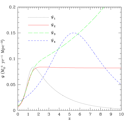
Figure 1: Cosmic star formation history as a function of redshift. Different linestyles correspond to the functions listed in equation (2.3).

2.3 Star formation history

In the past few years a number of authors have attempted to determine the star formation history of the universe from observational data. Although some details remain controversial, the evolution of the star formation rate (hereafter SFR) with redshift can be traced till to $z\sim 6$ using various diagnostics. It is widely accepted that for $z<1$ the SFR is a rapidly increasing function of redshift, reflecting the fact that present-day galaxies have been assembled long ago. Corrections for dust reddening and extinction complicate the picture at higher redshifts. To summarize the present knowledge and the corresponding uncertainty, we use here four different parameterizations of the global star-formation rate per unit comoving volume:

$$\psi_{1}(z) = 0.3\,\frac{h}{0.65}\,\frac{\exp(3.4\,z)}{\exp(3.8\,z)+45}\,\Upsilon(z)\,M_{\odot}\,{\rm yr}^{-1}\,{\rm Mpc}^{-3}\;,$$

$$\psi_{2}(z) = 0.15\,\frac{h}{0.65}\,\frac{\exp(3.4\,z)}{\exp(3.4\,z)+22}\,\Upsilon(z)\,M_{\odot}\,{\rm yr}^{-1}\,{\rm Mpc}^{-3}\;,$$ (6)

$$\psi_{3}(z) = 0.2\,\frac{h}{0.65}\,\frac{\exp(3.05\,z-0.4)}{\exp(2.93\,z)+15}\,\Upsilon(z)\,M_{\odot}\,{\rm yr}^{-1}\,{\rm Mpc}^{-3}\;,$$

$$\psi_{4}(z) = 0.15\,\frac{14\exp[0.6(z-5.4)]}{5+9\exp[0.933(z-5.4)]}\,M_{\odot}\,{\rm yr}^{-1}\,{\rm Mpc}^{-3}\;.$$

with

$$\Upsilon(z)=\frac{[\Omega_{0}\,(1+z)^{3}+\Omega_{k}\,(1+z)^{2}+\Lambda]^{1/2}}{(1+z)^{3/2}}\;.$$ (7)

The first three, obtained by Porciani & Madau [17], match present data from UV-continuum and H-$\alpha$ cosmic luminosity densities, and allow for different amounts of dust reddening, especially at high-$z$ (see Ref. [17] for further details). The fourth SFR is taken from Ref. [18] (see also [19]) and is based on theoretical speculation only. This is obtained from a set of cosmological simulations including gas hydrodynamics where an a priori recipe for star formation has been assumed. The whole analysis has been developed in the framework of a vacuum energy dominated cold dark matter model in which galaxies form hierarchically. At variance with the determinations based on observational data, this SFR extends to very high redshifts but suffers from a number of theoretical assumptions. The resulting function has a maximum at $z\sim 5.5$ and declines roughly exponentially towards both high and low redshifts. A semianalytic model to explain the origin of this functional form has been presented by Hernquist & Springel [20]. The SFRs given in equation (2.3) are plotted in Figure 1. The intensity of the cosmic neutrino background have been computed by integrating equation (4) out to $z_{\rm max}=10$.

2.4 Initial Mass Function

Basic reasoning suggests that the IMF should vary with the properties of the star-forming clouds. Nevertheless, although there is no fundamental reason for a universal mass distribution of stars, so far no firm evidence for a variable IMF exists (see e.g. Refs. [21, 22, 23] for different points of view regarding this issue). In what follows we will assume a time independent IMF, adopting different functional forms to take into account observational uncertainties. As a standard model we use the IMF originally proposed by Salpeter: $\phi(M)\propto M^{-2.35}$. Even though this is supported by many studies, especially for $M\gtrsim 0.5\,M_{\odot}$ (see e.g. [24, 25]), the behavior of the IMF at lower masses is still very uncertain (see e.g. [25, 26, 27]). This reflects the observational uncertainties in the determination of the star luminosity function at low luminosities. To represent a number of different observational results, we focus here on two additional examples. From M-dwarf observations with the Hubble Space Telescope, Gould, Bahcall & Flynn [28] determined the following form for the low-mass end of the IMF ($M<1.6M_{\odot}$):

$$\log(\phi)={\rm const.}-2.33\log(M/M_{\odot})-1.82\ [\log(M/M_{\odot})]^{2}\;.$$ (8)

This function peaks at $M\sim 0.23\,M_{\odot}$, and the slope at $M=1\,M_{\odot}$ is $-2.33$, almost coincident with the Salpeter value of $-2.35$. We will call GBF IMF the distribution obtained by matching this equation for $M<1\,M_{\odot}$ with a Salpeter IMF for higher masses. Finally, as a third option, we use a parameterization of the IMF obtained from star counts in different Galactic fields by Kroupa [25]. This is well fit by a broken power-law with a change in the exponent near $0.5\,M/M_{\odot}$, namely, $\phi\propto M^{-\alpha_{i}}$, with $\alpha_{1}=1.3$ for $M/M_{\odot}\leq 0.5$ and $\alpha_{2}=2.3$ for $M/M_{\odot}>0.5$. In all cases, we assume $M_{\rm min}=0.08\,M_{\odot}$ and $M_{\rm max}=125\,M_{\odot}$.

2.5 Results

In this section, we present our main results, obtained by combining in equation (4) the different functions discussed above. In Figure 2, the expected cosmic background intensity, $\bar{I}_{\nu}^{(0)}$, is plotted as a function of energy for different star formation histories and assuming a Salpeter IMF. The corresponding fluxes, integrated over all energies, are listed in Table 1.

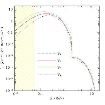
Figure 2: Mean intensity of the cosmic neutrino background as a function of energy. Different linestyles correspond to different assumed SFRs. We only consider neutrinos produced by thermonuclear reactions in stars. The shaded region highlights the energy range in which additional “cooling neutrinos” are expected to contribute significantly.

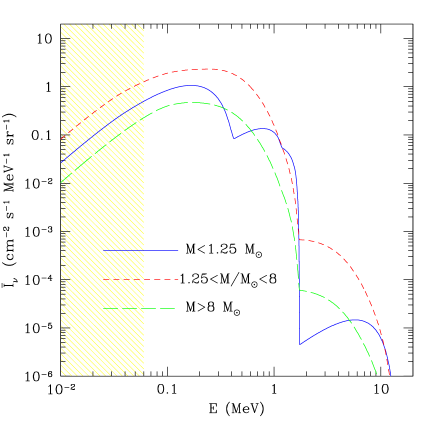
Figure 3: Contributions to the neutrino differential flux due to stars of different masses. A Salpeter IMF and $\psi_{2}(z)$ are assumed.

The amplitude of the background ranges within a factor of 2, with $\psi_{3}$ and $\psi_{1}$ giving the highest and the lowest fluxes, respectively. This is not surprising since $\psi_{1}$ has a much lower amplitude than the other SFRs at $z>2$, while $\psi_{3}$ keeps increasing with redshift. It is interesting to compare the contributions to the background due to low ($M/M_{\odot}<1.2$), intermediate ($1.2\leq M/M_{\odot}<8\,M_{\odot}$) and high mass stars ($M/M_{\odot}\geq 8$). This is done in Figure 3, where a Salpeter IMF and $\psi_{2}(z)$ are assumed. The shape of the different curves can be explained as follows. Very-low mass stars, $M/M_{\odot}\lesssim 0.9$, produce only pp neutrinos with energies below 0.4 MeV.

Table 1: Cosmic neutrino background.

SFR	IMF	$c\,n$	$n\cdot 10^{9}$	$u\cdot 10^{10}$	$\Omega_{\nu}\,h^{2}\cdot 10^{8}$	$\bar{E}$	$\bar{z}$	$s\cdot 10^{7}/k_{\rm b}$
		$({\rm cm}^{-2}\,{\rm s}^{-1})$	$({\rm cm}^{-3})$	$({\rm MeV}\,{\rm cm}^{-3})$		(MeV)		$({\rm cm}^{-3})$
1	Salp.	20.2	0.68	2.73	2.59	0.40	1.41	0.61
1	Kroupa	29.8	0.99	4.03	3.82	0.40	1.45	0.89
1	GBF	35.9	1.20	4.86	4.61	0.41	1.43	1.07
2	Salp.	26.0	0.87	3.29	3.12	0.38	1.83	0.77
2	Kroupa	38.2	1.27	4.81	4.57	0.38	1.88	1.13
2	GBF	46.1	1.54	5.85	5.55	0.38	1.86	1.36
3	Salp.	36.7	1.22	4.67	4.43	0.38	2.01	1.09
3	Kroupa	53.5	1.79	6.78	6.43	0.38	2.06	1.58
3	GBF	65.0	2.17	8.32	7.90	0.38	2.04	1.92
4	Salp.	21.2	0.71	2.56	2.43	0.36	2.30	0.63
4	Kroupa	31.3	1.04	3.78	3.59	0.36	2.36	0.93
4	GBF	37.6	1.26	4.57	4.34	0.36	2.33	1.11

Masses in the range $0.9\lesssim M/M_{\odot}\lesssim 1.2$ pass through the ppII and ppIII chains, thus emitting ⁷Be and ⁸B neutrinos. The small contribution of ⁸B neutrinos to the total flux is evident at higher energies. The peculiar feature at energies in the range $0.4\lesssim(E/1\ \mathrm{MeV})\lesssim 2$ is due to the reduced quantity of CNO neutrinos emitted by these stars during their H-burning shell phase. As discussed above, the stellar neutrino luminosity rapidly increases with mass and, in particular, the contribution of CNO, ⁸B, and ⁷Be neutrinos increases. Nevertheless, the steep slope of the IMF and the shorter main sequence lifetime diminish the contribution of massive stars to the stellar neutrino background.

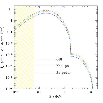
Figure 4: As in Fig. 1 but for different IMFs, assuming $\psi_{2}$ for the SFR.

In summary, intermediate mass stars clearly dominate the background at all energies but for a narrow window around 1.5 MeV where small mass stars give a slightly larger contribution. In Figure 4 we show how the spectrum of the background changes by varying the IMF while using the same SFR (in this case, $\psi_{2}$). The reader is referred to Table 1 for the corresponding fluxes. The net effect is a slight spectral distortion and a difference in the background intensity as large as a factor of 2. As expected, the amplitude of the background increases when the relative weight of low-mass stars is reduced.

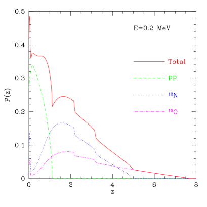
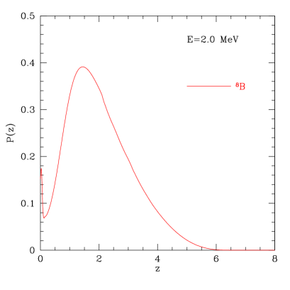
Figure 5: Probability distribution of the emission redshift for neutrinos with energy $E$ in the cosmic background (solid line). Different linestyles denote the contribution of different generation processes, namely: pp fusion (dashed), ¹³N decay (dotted), and ¹⁵O decay (dot-dashed). Left and right panels refer to $E=0.2$ MeV and $E=2$ MeV, respectively.

It is interesting to study how the the probability density distribution for the emission redshift of neutrinos varies with their energy at detection. This is simply given by

$$P(z,E)=\frac{c}{4\pi}\frac{\epsilon_{\nu}\left[E(1+z),z\right]}{H_{0}\,[\Omega_{0}(1+z)^{3}+\Omega_{k}(1+z)^{2}+\Omega_{\Lambda}]^{1/2}}\frac{1}{I_{\nu}^{(0)}(E)}\;,$$ (9)

and it is shown in Figure 5 for two different neutrino energies. Note that neutrinos at the peak of the energy spectrum ($E\simeq 0.2$ MeV) have been emitted within a wide redshift range. Three different generation mechanisms contribute: the nuclear fusion of 2 protons (which accounts for the 27 per cent of the neutrinos observed at $E=0.2$ MeV) and the $\beta^{+}$ decays of ¹³N (44 per cent) and ¹⁵O (29 per cent). Each of these processes corresponds to a different distribution of emission redshifts, which is determined by the joint effect of the SFR and the shape of the rest-frame emission spectrum. For instance, the narrow peak near $z=0$ is generated by stars with $M\simeq 1M_{\odot}$ which started to produce energy through the CNO cycle only recently. We find that the mean emission redshift for photons at $E=0.2$ MeV is $\bar{z}=1.83$. On the other hand, at higher energies, only the ⁸B $\beta^{+}$ decay contributes. The emission-redshift distribution for neutrinos at $E=2$ MeV is shown in the right panel of Figure 5. In this case, we find $\bar{z}=2.03$.

For $E<0.06$ MeV, the contribution to the total neutrino fluxes of cooling neutrinos should eventually be taken into account. In fact, the estimated neutrino fluxes at the Earth’s surface due to plasma-neutrinos emitted by stars till the end of the Red Giant phase as well as during the last phase of cooling as white dwarfs is comparable to the pp-neutrinos flux [9].

2.6 Cosmological relevance

It is interesting to compare the energy and entropy densities of neutrinos generated by thermonuclear reactions in the universe with the corresponding quantities for the primordial neutrino background. The present-day number and energy densities of the cosmic neutrino background generated by stars are

$$n=\frac{4\pi}{c}\int\bar{I}_{\nu}^{(0)}(E)\,dE\ \ \ \ \ \ {\rm and}\ \ \ \ \ \ u=\frac{4\pi}{c}\int E\,\bar{I}_{\nu}^{(0)}(E)\,dE\;,$$ (10)

respectively. We define the entropy density for our non-thermal cosmic neutrino background as

$$s=\frac{4\pi\,k_{\rm b}\,g_{\rm s}}{c^{3}\,h^{3}}\int_{0}^{\infty}E^{2}\left\{f(E)\ln\left[\frac{1}{f(E)}-1\right]-\ln\left[1-f(E)\right]\right\}dE\;,$$ (11)

where

$$f(E)=h^{3}\,c^{2}\,\frac{\bar{I}_{\nu}^{(0)}(E)}{E^{2}}\simeq 6.36\times 10^{-41}({\rm MeV}^{3}\,{\rm cm}^{2}\,{\rm s})\,\frac{\bar{I}_{\nu}^{(0)}(E)}{E^{2}}\;,$$ (12)

$k_{\rm b}$ denotes the Boltzmann constant, $g_{\rm s}$ is the number of helicity degrees of freedom, and $h$ is the Planck’s constant. This is derived from first principles in the Appendix and gives the standard result $s=4.202\,k_{\rm b}\,n$ for a thermal background. Note that, since neutrinos in the cosmic background are far from being degenerate (i.e. $f(E)\ll 1$), equation (11) reduces, in practice, to $s\propto-\int E^{2}\,f(E)\,\ln[f(E)]\,dE$. Values for the number, energy and entropy densities of the background are listed in Table 1 for the different models we considered. Typically, $n\simeq 10^{-9}\,{\rm cm}^{-3}$, $u\simeq 5\times 10^{-10}\,{\rm MeV\,cm}^{-3}$ (corresponding to a contribution to the density parameter of $\Omega_{\nu}\,h^{2}\simeq 5\times 10^{-8}$) and $s\simeq 10^{-7}\,k_{\rm b}\,{\rm cm}^{-3}$. On the other hand, from the standard theory of neutrino decoupling in the early universe one expects a thermal distribution of relic particles with $T_{\rm rel}=1.95$ K. This contributes $n_{\rm rel}=56.5\,{\rm cm}^{-3}$, $\Omega_{\rm rel}\,h^{2}\simeq 4.8\times 10^{-6}$ (for massless neutrinos), and $s_{\rm rel}=203.5\,k_{\rm b}\,{\rm cm}^{-3}$ for each neutrino family (an equal contribution is given by the corresponding antiparticles). We can thus draw the conclusion that thermonuclearly produced neutrinos hardly are of any cosmological relevance. In particular, their abundance and entropy are overwhelmed by the corresponding properties of relic neutrinos from the hot initial phases of the universe. However, since thermonuclear neutrinos from stars are characterized by much higher energies than the thermal relics from the big bang, the ratio of the energy densities of this two backgrounds is much smaller than the number density ratio. In both cases, the contribution to the curvature of space-time is anyway negligible.

2.7 Constraints on the neutrino radiative lifetime and electromagnetic form factors

In the hypothesis of radiative neutrino decay, $\nu\rightarrow\nu_{\ell}+\gamma$, cosmic neutrinos ($\nu$ with mass $m$) decaying into some neutral fermion (possibly a lighter neutrino $\nu_{\ell}$ with mass $m_{\ell}$) over a Hubble time would be the source of a diffuse photon background. For a fixed energy $E_{\nu}$ of the heavy neutrino, the photon spectrum is continuum, with an end point at $E_{\gamma}=E_{\nu}(m^{2}-m_{\ell}^{2})/m^{2}$ for ultrarelativistic neutrinos. Depending on the mass pattern, the photon energy can extend up to the MeV region. As derived in Appendix B, the background intensity of the resulting photons at $z=0$ is

$$j(E)=\frac{m\,c^{2}}{\tau_{\gamma}}\,\frac{\alpha(E)}{H_{0}\,E}\,\bar{I}_{\nu}^{(0)}(2E)\;,$$ (13)

where $\tau^{-1}_{\gamma}$ is the radiative decay rate and

$$\alpha(E)=\int_{0}^{\infty}\!\!\!\frac{dz}{(1+z)^{2}\,[\Omega_{0}(1+z)^{3}+\Omega_{k}(1+z)^{2}+\Omega_{\Lambda}]^{1/2}}\int_{z}^{\infty}\!\!\!dz^{\prime}\,P(z^{\prime},2E)\;,$$ (14)

a numerical coefficient of order unity.

Observations have shown the presence of a diffuse (high-latitude) photon background in the MeV region that appears to be of extragalactic origin. Both a large number of unresolved point sources and truly diffuse processes might potentially contribute. However, the X-ray background (below 100 keV) is generally understood to arise primarily from the integrated emission of active galactic nuclei (such as Seyfert galaxies) with redshifts ranging up to 6 [29]. At slightly higher energies ($E\sim 1$ MeV), radioactivity in Type Ia supernovae is expected to be the most important contributor [30].

The amplitude of the diffuse $\gamma$-ray background in the MeV range is extremely hard to measure (both from the Earth and from space) due to the extraordinarily high atmospheric and instrumental background. In particular, the interaction of cosmic rays with the detector and nuclear line emission dominate the noise. Recent results from a number of satellite missions indicate the presence of an extragalactic component significantly lower than previous measurements. The Medium Energy Detectors of the A4 experiment onboard the High Energy Astrophysics Observatory 1 (HEAO-1) measured a background intensity $j(E)=(2.62\pm 0.05)\times(E/0.1\,{\rm MeV})^{-2.75\pm 0.08}\,{\rm cm}^{-2}\,{\rm s}^{-1}\,{\rm MeV}^{-1}\,{\rm sr}^{-1}$ for $0.1\leq(E/1\,{\rm MeV})\leq 0.4$ [32]. The Imaging Compton Telescope (COMPTEL) on the Compton Gamma Ray Observatory (CGRO) showed that the diffuse background at $0.8\leq(E/1\,{\rm MeV})\leq 30$ is consistent with power-law extrapolation from the HEAO result at lower energies [32], and provided a new fitting formula $j(E)=(1.05\pm 0.2)\times 10^{-4}\,(E/5\,{\rm MeV})^{-2.4\pm 0.2}\,{\rm cm}^{-2}\,{\rm s}^{-1}\,{\rm MeV}^{-1}\,{\rm sr}^{-1}$ [33]. Finally, the Solar Maximum Mission $\gamma$-ray spectrometer (SMM/GRS) measured a signal for $0.3\leq(E/1\,{\rm MeV})\leq 8.5$ which is $\sim 20\%$ lower than the COMPTEL determination [34].

If one attributes a fraction $f$ of the diffuse background to cosmic neutrino radiative decay, one can derive a lower bound for the radiative decay lifetime, $\tau_{\gamma}$ (the total lifetime is obtained by multiplication with the branching ratio for the radiative channel),

$$\frac{\tau_{\gamma}}{m\,c^{2}}\geq\frac{(2-6)}{f}\times 10^{12}\,\,{\rm s}\,\,{\rm eV}^{-1}\;.$$ (15)

The radiative decay rate can be uniquely characterized by the magnetic and electric (dipole) transition moments, $\mu_{\nu\,\nu_{\ell}}$ and $\epsilon_{\nu\,\nu_{\ell}}$, through (e.g. [35])

$$\frac{1}{\tau_{\gamma}}=\frac{\mu_{\rm eff}^{2}}{8\pi}\;\,m^{3}\,\left(1-\frac{m_{\ell}^{2}}{m^{2}}\right)^{3}\;,$$ (16)

where $\mu_{\rm eff}^{2}=|\mu_{\nu\,\nu_{\ell}}|^{2}+|\epsilon_{\nu\,\nu_{\ell}}|^{2}$ and natural units ($\hbar=c=1$) have been adopted for convenience. Assuming a mass hierarchy $m\gg m_{\ell}$ and measuring the effective magnetic moment in units of the Bohr magneton, $\mu_{\rm B}$, this corresponds to

$$\frac{\mu_{\rm eff}}{\mu_{\rm B}}\leq(1-4)\times 10^{-7}\,f^{1/2}\,\left(\frac{m\,c^{2}}{\rm 1\ eV}\right)^{-2}\;.$$ (17)

Note that, for $m\,c^{2}\ll 1$ eV (the favored mass range from current experiments), the radiative decay channel is vastly phase-space suppressed, and the phase-space factor $m^{3}$ in equation (16) strongly reduces the strength of the limit on $\mu_{\rm eff}$. Anyway, even by assuming $f=1$, our upper bound is much more stringent than the limit $\mu_{\rm eff}/\mu_{\rm B}\leq 0.09\,(m\,c^{2}/1\ {\rm eV})^{-2}$ derived from the absence of decay photons of reactor $\bar{\nu}_{e}$ fluxes [36], and from the solar neutrino flux, $\mu_{\rm eff}/\mu_{\rm B}\leq 5\times 10^{-6}\,(m\,c^{2}/1\ {\rm eV})^{-2}$ [37]. However, most of the hard X-ray background (2-10 keV) has been recently resolved into discrete sources [38]. The data compilation by Moretti et al. [39] shows that 90-95% of the background can be ascribed to discrete source emission. Accounting for scattered light, the resolved fraction might even equal 99% of the total [40]. Active galactic nuclei may similarly contribute even at 100 keV [41]. Assuming $f\simeq 0.01$, makes our result comparable to the limit derived from the Supernova 1987A neutrino burst, $\mu_{\rm eff}/\mu_{\rm B}\leq 1.5\times 10^{-8}\,(m\,c^{2}/1\ {\rm eV})^{-2}$, (see Ref. [42] and references therein).

Our bound on $\mu_{\rm eff}$, however, is not competitive with other astrophysical determinations (see [44] for a comprehensive review) based, for instance, on plasmon decay in globular cluster stars ($\mu_{\rm eff}/\mu_{\rm B}\leq 3\times 10^{-12}$) [45], the observation of TeV $\gamma$-rays from Markarian 421 and 501 [46], helioseismology ($\mu_{\rm eff}/\mu_{\rm B}\leq 4\times 10^{-10}$) [44], and the primordial neutrino background ($\mu_{\rm eff}/\mu_{\rm B}\leq 10^{-11}\,(m\,c^{2}/1\ {\rm eV})^{-9/4}$) [47]. Laboratory limits on the diagonal and transition magnetic moments are typically obtained from measurements of the $\bar{\nu}\,e$ scattering cross section at low energy near a nuclear reactor. Current upper limits to the transition moments involving a particular flavor are: $\mu/\mu_{\rm B}\leq 1.0\times 10^{-10}$ for $\nu_{e}$ [48], $\mu/\mu_{\rm B}\leq 7.4\times 10^{-10}$ for $\nu_{\mu}$ [49], and $\mu/\mu_{\rm B}\leq 5.4\times 10^{-7}$ for $\nu_{\tau}$ [50].

3 Galactic neutrino background

Will we ever be able to detect the cosmic neutrino background generated by stars directly? Beyond technological issues related to the availability of detectors with the required sensitivity, one needs to worry about the presence of other backgrounds. It is straightforward to think of neutrinos generated by thermonuclear reactions taking place within the Galaxy, since it is expected to have a similar spectrum to the cosmic one. In this section we compute the basic properties of this new background and its directional dependence on the sky. For analytical convenience, we will use here a different parameterization of the star formation rate, $\widetilde{\psi}^{(j)}(t^{\prime})$, denoting the mass of gas converted into stars per unit time in a given galatic component (thin disk, thick disk, halo and bulge) labelled by the index $(j)$. The mean density of stars that are still thermonuclearly active today can then be expressed as

$$n_{\rm active}=\frac{\int_{M_{\rm min}}^{M_{\rm max}}\!dM\,\phi(M)\,\int_{t_{M}}^{t_{0}}dt^{\prime}\,\widetilde{\psi}^{(j)}(t^{\prime})}{\int_{M_{\rm min}}^{M_{\rm max}}\!dM\,M\,\phi(M)}\;,$$ (18)

where $t_{0}=14.5$ Gyr is the present cosmic age in the adopted cosmological model. Therefore, the mean neutrino rate presently emitted by a star in the component $(j)$ through the production channel $(i)$ is

$$G_{\nu}^{(i,j)}=\frac{\int_{M_{\rm min}}^{M_{\rm max}}\!dM\,\phi(M)\,\int_{t_{M}}^{t_{0}}dt^{\prime}\,\widetilde{\psi}^{(j)}(t^{\prime})\,L^{(i)}_{\nu}(M,t_{0}-t^{\prime})}{\int_{M_{\rm min}}^{M_{\rm max}}\!dM\,\phi(M)\,\int_{t_{M}}^{t_{0}}dt^{\prime}\,\widetilde{\psi}^{(j)}(t^{\prime})}\;,$$ (19)

where, once again, $t_{M}=\max[0,t(z)-t_{\rm life}(M)]$. Note that, being a mean quantity, $G_{\nu}^{(i,j)}$ does not depend on the overall normalization of the star-formation rate but only on its temporal evolution. We account for the geometric structure of the galaxy by introducing a set of functions, $n^{(j)}({\bf r}_{\rm g})$, which describe the present-day number density distributions of stars in the different galactic components as a function of the distance from the galactic centre. The differential neutrino flux detected on Earth is thus

$$I_{\nu}^{(0)}(\hat{\bf r},E)=\frac{1}{4\pi}\sum_{i,j}G_{\nu}^{(i,j)}\,S^{(i)}_{\nu}(E)\,\int dr\,n^{(j)}({\bf r}+{\bf r}_{0})\;,$$ (20)

where ${\bf r}$ denotes separations from Earth and ${\bf r}_{0}$ is our distance from the galactic centre.

In the last decades, accurate star count surveys, gas-dynamical and stellar-kinematics studies, and the analysis of near-infrared brightness maps allowed us to identify the main structural features of the Milky Way and to formulate a number of standard density laws to describe its populations. Recently, a series of technological improvements made possible a more accurate determination of the corresponding free parameters. In this section, we will use these results to estimate the intensity and directional dependence of the Galactic neutrino background. In particular, for the outer galaxy, we will use the results from the high-latitude star counts obtained by the Sloan Digital Sky Survey [51] and by Siegel et al. [52] which homogeneously cover nearly 279 and 15 square degrees, respectively. Given the level of uncertainty, the design of the models is deliberately simple. Typically they account for two double-exponential disks (a thin and a thick one), a spheroidal halo and a central bulge. Given the degree of approximation of our calculations, we neglect the spiral structure in the disk. The corresponding best-fitting parameters are listed in Table 2. The results are strikingly similar but for the scale height of the thick disk, which, however, is poorly determined in both cases. Note that these smooth models are far from being perfect, and neglect many detailed features of the stellar distribution in the Galaxy. For instance, the outer halo might not be smooth but be composed by overlapping streams of stars (e.g. [53]). In general, residuals show that these models systematically overpredict stellar densities towards the galactic centre and underpredict them in the outer galaxy [52].

Because of the lack of low-latitude data, these models constrain the inner structure of the Galaxy only weakly. For instance, Siegel et al. [52] assume an $r^{-3}$ density distribution for the bulge, while it has long been known that the central region of the Galaxy has a distinct stellar density profile that approximately follows an $r^{-2}$ law (e.g. [54]). Recently, it has become widely accepted that our Galaxy is barred, as evidence accumulated over the last few years from a number of different observations. Along this line, a more accurate model for the light distribution in the inner Galaxy has been extracted by Binney, Gerhardt & Spergel [55] from the analysis of dust-corrected maps of the near-infrared brightness emission of the Galaxy (see e.g. [56]). The corresponding parameters are listed in Table 2. However, converting near-IR brightness maps into stellar densities its not an easy task since one has first to assume a mass-to-light ratio for the different components and then a stellar mass function. All these steps have a rather large error, and this leads to a large uncertainty in the final result. On the other hand, one could think about relating IR emission directly to either stellar density or, even, to neutrino luminosity. However, one needs to remember that a significant fraction of the IR brightness comes from dust and gas. Moreover, during the evolution out of the MS, the neutrino emission rate does not correlate anymore with the photon luminosity of a star, since the only source of thermo-nuclear neutrinos is a H burning shell, while the structure is partially supported by the triple $\alpha$ reactions. For simplicity, we assumed a constant conversion factor between infrared brightness and stellar number density in the different components. In the end, in order to bracket our predictions for the Galactic neutrino background, we combine the data listed in Table 2 into two distinct models. The first one (G1) is completely based on the results by Siegel et al. [52] and it is expected to give the highest neutrino flux. The second model (G2) is instead obtained by combining the disk+bulge fit by Binney et al. [55] with the halo+thick disk results by Chen et al. [51]. In both cases, whenever a given parameter is associated with a finite range of values in Table 2, we assumed the mean value of the quoted extremals. Both models are normalized by imposing that the number density of stars in the solar neighborhood belonging to the thin disk is 0.1 pc^-3 [57]. Moreover, in order to avoid unphysical divergences, we adopt a constant density distribution within the inner 20 pc of the bulge (in G1) and within the inner 240 pc of the halo (in both G1 and G2).

Table 2: Structure parameters in the adopted Galaxy models

Parameter	Binney et al. (1997)	Chen et al. (2001)	Siegel et al. (2002)
Disk density law	Double exponential	Double exponential	Double exponential
Disk scale length (pc)	2500	2250	2000-2500
Disk scale height (pc)	210 + 42	330	350
Disk local normalization (pc-3)	0.1	0.1	0.1
Thick-disk density law		Double exponential	Double exponential
Thick-disk scale length (pc)		3500	3000-4000
Thick-disk scale height (pc)		580-750	900-1200
Thick-disk/disk local
normalization (%)		6.5-13	6-10
Halo density law		Power law	Power law
Halo power-law index		2.5	2.75
Halo axial ratios $(b/a,c/a)$		(1,0.55)	(1,0.5-0.7)
Halo/disk local normalization (%)		0.125	0.15
Bar/Bulge density law	Exp-truncated power-law		Power-law
Bar/Bulge axial ratios $(b/a,c/a)$	$(0.5,0.6)$		$(1,0.5)$
Bar/Bulge power-law index	1.8		3
Bar/Bulge scale length (pc)	1900
Bar/Bulge core size (pc)	100
Angle between the Bar/Bulge	$20^{\circ}$
major axis and the Sun-centre line
Bulge/disk local normalization (%)	$6.1\times 10^{-13}$		0.02
Solar distance
from the Galactic centre (pc)	8000	8000	8000
Solar distance
from the Galactic mid-plane (pc)	14	27	15

No compelling constraints currently exist on the star formation histories of the various galactic components. We adopt an overall picture based on the studies by Binney, Dehnen, & Bertelli [58] and Liu & Chaboyer [59]. In particular, we assume that the thin disk started forming 11.2 Gyr ago (which correspond to $z\simeq 2.1$ in our cosmological model) and kept forming stars at the same pace till to the present epoch. This is consistent with present data and with the assumption of a Salpeter IMF [58]. Note, however, that the slope of the initial mass function near $1\,M_{\odot}$ proves to be degenerate with the rate at which the star formation rate declines. We assume a synchronous formation of the galactic halo which dates back to 12.2 Gyr ago ($z\simeq 3$), and a constant SFR in the thick disk lasting from 12.2 to 11.2 Gyr. As regards the bulge, recent HST/WFPC2 [60] and near-IR data [61] seem to suggest that it is coeval with the halo and that no significative amount of new stars formed after the intense initial starburst activity.

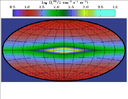
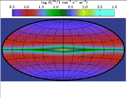
Figure 6: Aitoff projection of the intensity of the Galactic neutrino background on the sky. Color coding scales logarithmically with the background intensity, and Galactic coordinates are used. Left and right panels refer to model G1 and G2, respectively.

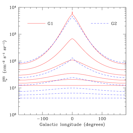
Figure 7: The Galactic neutrino background intensity as a function of direction of observation on the sky. Different lines show the $\ell$ dependence at fixed latitude $b$. From top to bottom, $b=0^{\circ},6^{\circ},15^{\circ},30^{\circ},45^{\circ},90^{\circ}$. Continuous lines refer to model G1, while dashed lines are for G2.

Sky-maps of the Galactic neutrino background intensity are shown in Figure 6. To facilitate a quantitative reading of the plots, in Figure 7, the background intensity is plotted as a function of Galactic longitude for a number of 1D-cuts at fixed latitude. Both figures have been obtained by integrating $I_{\nu}^{(0)}(\hat{\bf r},E)$ over the particle energy, keeping $\hat{\bf r}$ fixed. Note the spike in the background intensity towards the galactic centre, caused by the extreme stellar densities in the bulge. Independently of the Galaxy model, the amplitude of the neutrino background varies by roughly 3 orders of magnitude between the Galactic centre and the high-latitude isotropic component. Because of this large variation, all the different structural component of the Galaxy are clearly discernible from the maps. The amplitude of the high-latitude Galactic signal is always larger than the cosmic background (by a factor of a few in G1 and by roughly an order of magnitude in G2). This makes the detection of the cosmic background extremely difficult.

Integrating the background over the whole sky, one obtains a neutrino flux of 943 ${\rm cm}^{-2}\,{\rm s}^{-1}$, for model 1, and 333 ${\rm cm}^{-2}\,{\rm s}^{-1}$, for model 2. The corresponding energy spectra are shown in Figure 8. In Table 3 we list the contributions to the flux from the different structural components of the Galaxy. At every latitude, the counts are dominated by neutrinos emitted in the Galactic disk which, independently of the Galaxy model considered, account for more than 95 per cent of the total.

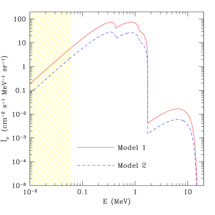
Figure 8: Energy spectrum of the Galactic neutrino background averaged over the whole sky.

Table 3: Galactic neutrino background.

Galaxy model	Total	Thin disk	Thick disk	Halo	Bulge
	$({\rm cm}^{-2}\,{\rm s}^{-1})$	$({\rm cm}^{-2}\,{\rm s}^{-1})$	$({\rm cm}^{-2}\,{\rm s}^{-1})$	$({\rm cm}^{-2}\,{\rm s}^{-1})$	$({\rm cm}^{-2}\,{\rm s}^{-1})$
1	943	923	17.4	1.72	0.66
2	333	314	15.3	1.12	3.17

4 Concluding Remarks

We have estimated two neutrino backgrounds on the sky, in the 50 keV-10 MeV window: the Galactic component from stars presently burning Hydrogen and Helium in the Milky Way and the cosmic contribution from thermonuclear reactions in other galaxies. On the grounds of the recent findings of Super-Kamiokande, SNO, and KamLAND, these neutrinos, born as $\nu_{e}$, propagate as a superposition of (at least) two mass eigenstates. When (and if) interacting with matter, they will show up as neutrinos of all flavors, with comparable probabilities.

Depending only slightly on some model details (namely, the assumed functional form of the SFR and the IMF), the background intensity of the cosmic component peaks at $E\simeq 0.1-0.3$ MeV, where $\bar{I}^{(0)}_{\nu}=3-7\,{\rm cm}^{-2}\,{\rm s}^{-1}\,{\rm MeV}^{-1}\,{\rm sr}^{-1}$, and sharply drops by 2 orders of magnitude above 1-2 MeV. The corresponding flux at the Earth’s surface (integrated over all energies) ranges between 20 and 65 ${\rm cm}^{-2}\,{\rm s}^{-1}$, while the associated energy density is $\simeq 5\times 10^{-4}\,{\rm eV}\,{\rm cm}^{-3}$. Assuming that the sum of the masses of the three neutrino flavors is at least 1/30 eV (as suggested by the oscillation patterns of solar and atmospheric neutrinos) implies that this energy density is negligibly small with respect to the contribution from the thermal ($T_{\rm rel}=1.95$ K) background of relic neutrinos originated in the early universe ($u_{\rm rel}>3.7\,{\rm eV}\,{\rm cm}^{-3}$). Similarly, the number and entropy densities of cosmic thermonuclear neutrinos ($n\simeq 10^{-9}\,{\rm cm}^{-3}$, $s\simeq 10^{-7}\,k_{\rm b}\,{\rm cm}^{-3}$) are overwhelmed by the corresponding quantities for the primordial background ($n_{\rm rel}\simeq 10^{2}\,{\rm cm}^{-3}$, $s_{\rm rel}\simeq 10^{3}\,k_{\rm b}\,{\rm cm}^{-3}$).

Thermonuclear neutrinos reaching the Earth today have been typically produced by stars around $z\sim 2$. Even though they have been around for a significant fraction of the life of the universe, they hardly interacted with anything. As far as we know, the thermonuclear neutrino background is absolutely transparent to any diffuse radiation impinging onto it since the mean free path $\lambda=(n\,\sigma)^{-1}$ exceeds the Hubble length for any reasonable value for the interaction cross section $\sigma$.

Attributing a fraction $f$ of the observed $\gamma$-ray background in the sub-MeV region to neutrino radiative decay, one can derive a lower bound for the radiative lifetime, valid for any neutrino type and mass $m$, $\tau_{\gamma}/m\geq(2-6)\,f^{-1}\times 10^{12}$ s ${\rm eV}^{-1}$. This can be easily translated into a limit for the electromagnetic form factors, which, after accounting for the contribution of active galactic nuclei (i.e. by assuming $f\sim 10^{-2}$), is competitive with the results obtained from the analysis of the SN1987A neutrino burst.

Independently of the direction of observation on the sky, the Galactic thermonuclear background dominates its cosmic counterpart. Even at high latitudes, Galactic neutrinos outnumber the cosmological background by a factor which ranges between a few and 10 depending on the details of the Galaxy model (see Figures 6 and 7). The integrated flux of Galactic neutrinos over the whole sky ranges between 300 and 1000 ${\rm cm}^{-2}\,{\rm s}^{-1}$. The emission from stars in the Galactic disk contributes more than 95 per cent of the signal.

Is there any prospect for detecting the Galactic component and, in the long term, to derive an observational neutrino map of the Galaxy? This clearly requires directional detectors, since one has first to distinguish the Galactic neutrino flux from the solar component. In the last ten years, large Cherenkov detectors have been built and successfully operated (Kamiokande, Super-Kamiokande and SNO), recording the directional signal of target electrons scattered from the impinging neutrinos. Analyzing the angular distribution of the events with respect to the Sun direction, the peak due to solar neutrinos is clearly discernible over a flat background [62]. So far, this method has been applied to the detection of the most energetic solar neutrinos originating from Boron decay (corresponding to a measured flux of $2.4\times 10^{6}\,{\rm cm}^{-2}\,{\rm s}^{-1}$). In this case, the decay of ²²²Rn in water, natural radioactivity, reactor antineutrinos, and radioactive decay of muon induced spallation products account for most of the instrumental background. After applying all possible cuts, background counts above 5 MeV are about ten times the number of events from solar neutrinos. Even though this is not the optimal energy window for the detection of Galactic neutrinos, it is interesting to note that, for $E_{\nu}>5$ MeV, their flux amounts to $\sim 1$ cm^-2 s^-1, which is nearly 7 orders of magnitude smaller than the instrumental background. This shows how far we are from their detection.

Dedicated experimental designs and techniques should then be devised to detect cosmic and Galactic neutrinos. Let us consider, for instance, the cosmic (anti)neutrino background from Type II supernovae. Kaplinghat et al. [5] found an upper bound to the flux of 54 cm^-2 s^-1 while, more recently, Ando, Sato, & Totani [6] estimate $c\cdot n\simeq 11$ cm^-2 s^-1. Even though there is no energy region in which the contribution from supernova neutrinos dominates over the backgrounds, their presence might be detectable with Cherenkov telescopes as a distortion in the spectrum of electron and positrons produced in the decay of invisible muons. Ten years of integration at SuperKamiokande (or one at the proposed HyperKamiokande) should already guarantee a $1\,\sigma$ detection of the supernova neutrino background at $\sim 20$ MeV [6].

Over the next decade, the focus of solar neutrino experiments will shift gradually from the relatively high energy ⁸B neutrinos to the low energy, ⁷Be, p-p, and CNO neutrinos. This is an encouraging perspective for the detection of a Galactic signal since, for $E<15$ MeV, the number density of thermonuclear neutrinos in the cosmic and Galactic backgrounds is expected to exceed that generated by Type II supernovae. Regrettably, instrumental backgrounds tend to increase in the MeV region. Therefore, in order to use the solar neutrino experiments to measure a Galactic signal, it is mandatory to suppress the noise in the detectors by several orders of magnitude by using more efficient screening procedures and accurate selection of radiopure materials. Note that extremely long times of integration might be anyway necessary to detect Galactic neutrinos with high statistical significance.

In summary, thermonuclear reactions in the Galaxy produce an anisotropic neutrino background in the MeV region. At the Earth’s surface, this corresponds to an integrated flux of $\sim 1000\ {\rm cm}^{-2}\,{\rm s}^{-1}$. Even though current detectors are unable to distinguish this signal from other backgrounds, it is not inconceivable that Galactic neutrinos might be revealed in the relatively near future with dedicated experimental setups.

Appendix A Entropy of a fermionic system

Fermions have antisymmetric wavefunctions under particle exchange and this implies that no two fermions can exist in the same quantum state (Pauli exclusion principle). The number of ways an energy level $E_{i}$ corresponding to $g_{i}$ degenerate quantum states can be populated with $n_{i}$ fermions is given by the binomial distribution with $g_{i}$ boxes, where $n_{i}$ contain 1 particle and $g_{i}-n_{i}$ are empty, i.e.

$$\frac{g_{i}!}{n_{i}!\,(g_{i}-n_{i})!}\;.$$ (21)

Allowing for a system with different energy levels, the total number of configurations is

$$W(\{n_{i}\})=\prod_{i}\frac{g_{i}!}{n_{i}!\,(g_{i}-n_{i})!}\;.$$ (22)

We define the entropy of the system as

$$S = k_{\rm b}\ln W(\{n_{i}\})\simeq$$

$$\simeq k_{\rm b}\sum_{i}\left\{g_{i}(\ln g_{i}-1)-n_{i}(\ln n_{i}-1)-(g_{i}-n_{i})[\ln(g_{i}-n_{i})-1]\right\}\;,$$

where, assuming both $n_{i}$ and $g_{i}$ are $\gg 1$, we used Stirling’s approximation $\ln n!\simeq n\,(\ln n-1)$. The problem with eq.(A) is that it requires knowledge of the whole set $\{n_{i}\}$, which, in practice, is a formidable task. A standard approximation is to replace $W(\{n_{i}\})$ with $W(\{\bar{n}_{i}\})$ (where $\bar{n}_{i}$ denotes the mean occupation number of the energy level $E_{i}$) in the above definition of entropy. In this case, neglecting 1 compared to $g_{i}$, one gets

$$S=k_{\rm b}\sum_{i}\left[\bar{n}_{i}\ln\left(\frac{g_{i}}{\bar{n}_{i}}-1\right)-g_{i}\ln\left(1-\frac{\bar{n}_{i}}{g_{i}}\right)\right]\;.$$ (24)

It is convenient to introduce the mean occupation number of a single quantum state $f_{i}=\bar{n}_{i}/g_{i}$ to obtain

$$S=k_{\rm b}\sum_{i}g_{i}\left[f_{i}\ln\left(\frac{1}{f_{i}}-1\right)-\ln\left(1-f_{i}\right)\right]\;.$$ (25)

If the energy levels of the system are closely spaced, one may replace the discrete probability density $f_{i}$ by a continuous function $f(E)$. This is easily done for a set of free particles moving in an (essentially) infinite volume. In this case, all the sums over the energy levels $\sum_{i}g_{i}\dots$ may be replaced by integrals over the accessible phase-space volume $\int\dots d\Gamma/h^{3}$ with $d\Gamma=d^{3}q\,d^{3}p$. For ultra-relativistic particles, for which $E=c\,p$, the entropy per unit volume is then given by:

$$s=\frac{4\pi\,k_{\rm b}\,g_{\rm s}}{c^{3}\,h^{3}}\int_{0}^{\infty}E^{2}\left\{f(E)\ln\left[\frac{1}{f(E)}-1\right]-\ln\left[1-f(E)\right]\right\}dE\;,$$ (26)

with $g_{\rm s}$ the number of helicity degrees of freedom. This can be expressed in terms of the particle number density,

$$n=\frac{4\pi\,g_{\rm s}}{c^{3}\,h^{3}}\int_{0}^{\infty}E^{2}\,f(E)\,dE\;,$$ (27)

as

$$s=\chi\,k_{\rm b}\,n\;,$$ (28)

with

$$\chi=\frac{\int_{0}^{\infty}E^{2}\left\{f(E)\ln\left[f(E)^{-1}-1\right]-\ln\left[1-f(E)\right]\right\}dE}{\int_{0}^{\infty}E^{2}\,f(E)\,dE}$$ (29)

a dimensionless coefficient.

Appendix B Photon Spectrum from Radiative Decays

Let us assume that a set of cosmological sources produce neutrinos with a rate $\dot{n}_{\nu}(z)$ (particles per unit comoving volume per unit time) and with a redshift dependent energy spectrum $S(E_{\nu},z)$ (normalized to unity). Then, the differential comoving neutrino number density per unit energy at redshift $z$ is given by

$$\frac{dn_{\nu}}{dE_{\nu}} (E_{\nu},z)=\int_{z}^{\infty}\!\!\!\dot{n}_{\nu}(z^{\prime})\,S\left(\frac{E_{\nu}(1+z^{\prime})}{1+z},z^{\prime}\right)\frac{1+z^{\prime}}{1+z}\left|\frac{dt}{dz^{\prime}}\right|\,dz^{\prime}$$

$$= \frac{1}{H_{0}\,(1+z)}\int_{z}^{\infty}\!\!\!S\left(\frac{E_{\nu}(1+z^{\prime})}{1+z},z^{\prime}\right)\frac{\dot{n}_{\nu}(z^{\prime})\,dz^{\prime}}{[\Omega_{0}\,(1+z^{\prime})^{3}+\Omega_{k}\,(1+z^{\prime})^{2}+\Omega_{\Lambda}]^{1/2}}\;.$$

If neutrinos of energy $E_{\nu}$ decay radiatively with a (rest-frame) lifetime $\tau_{\gamma}\gg H_{0}^{-1}$, the decay rate in the cosmic frame will be $n_{\nu}(z)/\gamma(E_{\nu})\,\tau_{\gamma}$, where the Lorentz factor $\gamma(E_{\nu})=E_{\nu}/m_{\nu}\,c^{2}$. Assuming that the secondary neutrino is very light compared to the parent one implies that the decay photons have $E\simeq E_{\nu}/2$, so that the decay processes will produce a photon background with present-day intensity:

$$j(E)=\frac{c}{4\pi}\int_{0}^{\infty}\!\!\!dz\,(1+z)\int_{0}^{\infty}\!\!\!\frac{dE_{\nu}}{\gamma(E_{\nu})\,\tau_{\gamma}}\frac{dn_{\nu}}{dE_{\nu}}(E_{\nu},z)\,\delta_{D}\left(E(1+z)-\frac{E_{\nu}}{2}\right)\left|\frac{dt}{dz}\right|\;.$$ (31)

Inserting equation (B) into equation (31) and integrating over the Dirac-delta distribution, one eventually gets

$$j(E)=\frac{c}{4\pi}\,\frac{m_{\nu}c^{2}}{\tau_{\gamma}}\,\frac{1}{H_{0}^{2}\,E}\,\int_{0}^{\infty}\!\!\!\frac{dz}{(1+z)^{2}\,K(1+z)}\int_{z}^{\infty}\!\!\!dz^{\prime}\,\frac{\dot{n}_{\nu}(z^{\prime})\,S(2E(1+z^{\prime}),z^{\prime})}{K(1+z^{\prime})}\;,$$ (32)

with $K(x)=[\Omega_{0}\,x^{3}+\Omega_{k}\,x^{2}+\Omega_{\Lambda}]^{1/2}$. In Section 2.7, we used this expression to constrain the neutrino decay time.

Considering, for simplicity, a redshift-independent, monochromatic neutrino spectrum at emission, $S(E_{\nu},z)=\delta_{D}(E_{\nu}-E_{0})$, the neutrino energy distribution reduces to

$$\frac{dn_{\nu}}{dE_{\nu}}(E_{\nu},z)=\begin{cases}\displaystyle{\frac{E_{\nu}^{1/2}\,\dot{n}_{\nu}([E_{0}(1+z)/E_{\nu}]-1)}{H_{0}\,[\Omega_{0}\,E_{0}^{3}\,(1+z)^{3}+\Omega_{k}\,E_{\nu}\,E_{0}^{2}\,(1+z)^{2}+\Omega_{\Lambda}\,E_{\nu}^{3}]^{1/2}}}&\text{for}\quad E_{\nu}\leq E_{0}\\ 0&\text{for}\quad E_{\nu}>E_{0}\end{cases}$$ (33)

where cosmological expansion smeared the energy of neutrinos into a continuous spectrum. Similarly, for the photon background intensity, one gets

$$j(E)=\begin{cases}\displaystyle{\frac{c}{4\pi}\,\frac{1}{2}\,\frac{m_{\nu}c^{2}}{\tau_{\gamma}}\,\frac{\,\dot{n}_{\nu}(\tilde{z}(E))}{H_{0}^{2}\,E^{2}\,K(E_{0}/2E)}\,\int_{1}^{E_{0}/2E}\!\!\!\!\!\!\!\frac{dw}{w^{2}\,K(w)}}&\text{for}\quad E_{\nu}\leq E_{0}/2\\ 0&\text{for}\quad E_{\nu}>E_{0}/2\end{cases}$$ (34)

with $\tilde{z}(E)=(E_{0}/2E)-1$. For an Einstein-de Sitter universe ($\Omega_{0}=1,\Omega_{\Lambda}=0$), this becomes

$$j(E)=\begin{cases}\displaystyle{\frac{c}{4\pi}\,\frac{2^{3/2}}{5}\frac{m_{\nu}c^{2}}{\tau_{\gamma}}\,\frac{\dot{n}_{\nu}(\tilde{z}(E))}{H_{0}^{2}\,E_{0}^{2}}\,\left(\frac{E_{0}}{E}\right)^{1/2}\,\left(1-\left(\frac{2E}{E_{0}}\right)^{5/2}\right)}&\text{for}\quad E\leq E_{0}/2\\ 0&\text{for}\quad E>E_{0}/2\end{cases}$$ (35)

with $j(E)\propto E^{-1/2}$ for $E\ll E_{0}$. On the other hand, an empty universe ($\Omega_{0}=\Omega_{\Lambda}=0$) would give

$$j(E)=\begin{cases}\displaystyle{\frac{c}{4\pi}\,\frac{1}{2}\,\frac{m_{\nu}c^{2}}{\tau_{\gamma}}\,\frac{\dot{n}_{\nu}(\tilde{z}(E))}{H_{0}^{2}\,E_{0}^{2}}\,\left(\frac{E_{0}}{E}\right)\,\left(1-\left(\frac{2E}{E_{0}}\right)^{2}\right)}&\text{for}\quad E\leq E_{0}/2\\ 0&\text{for}\quad E>E_{0}/2\end{cases}$$ (36)

Finally, the effect of a non-vanishing cosmological constant can be sketched by looking at a de Sitter universe ($\Omega_{0}=0,\Omega_{\Lambda}=1$)

$$j(E)=\begin{cases}\displaystyle{\frac{c}{4\pi}\,\frac{1}{2}\frac{m_{\nu}c^{2}}{\tau_{\gamma}}\,\frac{\dot{n}_{\nu}(\tilde{z}(E))}{H_{0}^{2}\,E_{0}^{2}}\,\left(\frac{E_{0}}{E}\right)^{2}\,\left(1-\left(\frac{2E}{E_{0}}\right)\right)}&\text{for}\quad E\leq E_{0}/2\\ 0&\text{for}\quad E>E_{0}/2\;.\end{cases}$$ (37)

References

-
[1]
J. N. Bahcall, Phys. Rev. C 65 (2002) 015802;
R. Davis, Reviews of Modern Physics 75 (2003) 985. -
[2]
Q. R. Ahmad et al. (the SNO Collaboration), Phys. Rev.
Lett. 87 (2001) 071301;
Q. R. Ahmad et al. (the SNO Collaboration), Phys. Rev. Lett. 89 (2002) 011301 - [3] K. Eguchi et al. (the KamLAND Collaboration), Phys. Rev. Lett. 90 (2003) 021802
- [4] D. Hartmann, S. E. Woosley, Astropart. Phys. 7 (1997) 137
- [5] M. Kaplinghat, G. Steigman, T. P. Walker, Phys. Rev. D 62 (2000) 3001
- [6] S. Ando, K. Sato, T. Totani, Astropart. Phys. 18 (2003) 307
- [7] S. Nagataki, K. Kohri, S. Ando, K. Sato, Astropart. Phys. 18 (2003) 551
- [8] Hartmann, D., Meyer, B. S., Clayton, D. D., Luo, N., & Krishnan, T., in AIP Conf. Ser. 327, Nuclei in the Cosmos III, ed. M. Busso, C. M. Raiteri, and R. Gallino (New York: American Institute of Physics Press) (1995) 447
- [9] E. Brocato, V. Castellani, S. degl’Innocenti, G. Fiorentini, G. Raimondo, A&A 333 (1998) 910
- [10] M. Tegmark. et al., submitted to Phys. Rev. D (2003) (astro-ph/0310723)
- [11] J. N. Bahcall, Phys. Rev. D 44 (1991) 1644
- [12] J. N. Bahcall, Phys. Rev. D 49 (1994) 3923
- [13] J. N. Bahcall, Phys. Rev. C 56 (1997) 3391
- [14] J. N. Bahcall, R. K. Ulrich, Rev. Mod. Phys. 60 (1988) 297
- [15] J. N. Bahcall, Phys. Rev. C 54 (1996) 411
- [16] P. J. Schinder, D. N. Schramm, P. J. Wiita, S. H. Margolis, D. L. Tubbs, ApJ 313 (1987) 531
- [17] C. Porciani, P. Madau, ApJ 548 (2001) 522
- [18] V. Springel, L. Hernquist, MNRAS 339 (2003) 312
- [19] K. Nagamine, M. Fukugita, R. Cen, J. P. Ostriker, ApJ 558 (2001) 497
- [20] L. Hernquist, V. Springel, MNRAS 341 (2003) 1253
- [21] F. Eisenhauer, in Proceedings of a Workshop held at Ringberg Castle, Starburst Galaxies: Near and Far, ed. L. Tacconi and D. Lutz (Heidelberg: Springer-Verlag) 24 (2001)
- [22] G. Gilmore, in Proceedings of a Workshop held at Ringberg Castle, Starburst Galaxies: Near and Far, ed. L. Tacconi and D. Lutz (Heidelberg: Springer-Verlag) 34 (2001)
- [23] P. Kroupa, Science 295 (2002) 82
- [24] P. Massey, K. E. Johnson, K. Degioia-Eastwood, ApJ 454 (1995) 151
- [25] P. Kroupa, MNRAS 322 (2001) 231
- [26] J. Scalo, ASP Conference Series 142 (1998) The Stellar Initial Mass Function, ed. G. Gilmore and D. Howell, 201
- [27] C. Reylé, A. C. Robin, Ap&SS 281 (2002) 115
-
[28]
A. Gould, J. N. Bahcall, C. Flynn, ApJ 465 (1996) 759
A. Gould, J. N. Bahcall, C. Flynn, ApJ 482 (1997) 913 -
[29]
D. Leiter, E. Boldt, ApJ 260 (1982) 1
A. Comastri, G. Setti, G. Zamorani, G. Hasinger, A&A 296 (1995) 1 - [30] K. Watanabe, D. H Hartmann, M. D. Leising, L. S. The, ApJ 516 (1999) 285
- [31] R. L Kinzer, G. V. Jung, D. E. Gruber, J. L. Matteson, L. E. Peterson, ApJ 475 (1997) 361
- [32] S. C. Kappadatah et al., A&AS 120 (1996) 619
- [33] S. C. Kappadath, Ph.D. Thesis: Measurement of the Cosmic Diffuse Gamma-Ray Spectrum from 800 keV to 30 MeV, (Durham: University of New Hampshire) (1998)
- [34] K. Watanabe, M. D. Leising, G. H. Share, R. L. Kinzer, in AAS Bulletin of the American Astronomical Society 28 (1996) 189th AAS Meeting, (Washington DC: American Astronomical Society), 1308, ApJ 516 (1999) 285
- [35] R. N. Mohapatra, P. Pal, Massive Neutrinos in Physics and Astrophysics, (World Scientific, Singapore, 1991)
- [36] L. Oberauer, F. von Feilitzsch, R. L. Mössbauer, Phys. Lett. B 198 (1987) 113
- [37] G. G. Raffelt, Phys. Rev. D 31 (1985) 3002
- [38] R. F. Mushotzky, L. L. Cowie, A. J. Barger, K. A. Arnaud, Nature 404 (2000) 459
- [39] A. Moretti, S. Campana, D. Lazzati, G. Tagliaferri, ApJ 588 (2003) 696
- [40] A. M. Soltan, A&A 408 (2003) 39
- [41] A. A. Zdziarski, P. T. Zycki, J. H. Krolik, ApJ 414 (1993) L81
- [42] L. Oberauer, C. Hagner, G. G. Raffelt, E. Rieger, Astropart. Phys. 1 (1993) 377
-
[43]
R. Barbieri, R. N. Mohapatra, Phys. Rev. Lett. 61
(1988) 27
A. Ayala, J. C. D’olivo, M. Torres, Phys. Rev. D 59 (1999) 111901 -
[44]
G. G. Raffelt, Phys. Rep. 320 (1999) 319
G. G. Raffelt, Phys. Rep. 333 (2000) 593 - [45] M. Haft, G. G. Raffelt, A. Weiss, ApJ 425 (1994) 222
- [46] S. D. Biller et al., Phys. Rev. Lett. 80 (1998) 2992
- [47] M. T. Ressel, M. S. Turner, Comments Astrophys. 14 (1990) 323
-
[48]
Z. Daraktchieva et al. (the MUNU Collaboration),
Phys. Lett. B 564 (2003) 190
U. B. Li et al. (the TEXONO Collaboration) 2003, Phys. Rev. Lett., 90, 131802 - [49] D. A. Krakauer et al., Phys. Lett. B 252 (1990) 177
- [50] A. M. Cooper-Sarkar et al., Phys. Lett. B 280 (1992) 153
- [51] B. Chen et al. (the SDSS Collaboration), ApJ 553 (2001) 184
- [52] M. H. Siegel, S. R. Majewski, I. N. Reid, I. B. Thompson, ApJ 578 (2002) 171
- [53] R. A. Ibata, G. F. Lewis, M. J. Irwin, T. Quinn, MNRAS 332 (2002) 915
- [54] E. E. Becklin, G. Neugebauer, ApJ 151 (1968) 145
- [55] J. J. Binney, O. E. Gerhard, D. N. Spergel, MNRAS 288 (1997) 365
- [56] E. Dwek et al., ApJ 451 (1995) 188
- [57] H. Jahreiss, R. Wielen, in ESA SP-402, Hipparcos ’97. Presentation of the Hipparcos and Tycho catalogues and first astrophysical results of the Hipparcos space astrometry mission, ed. B. Battrick, M.A.C. Perryman and P.L. Bernacca, (Noordwijk: ESA) (1997) 675
- [58] J. Binney, W. Dehnen, G. Bertelli, MNRAS 318 (2000) 658
- [59] W. M. Liu, B. Chaboyer, ApJ 544 (2000) 818
- [60] G. Feltzing, G. Gilmore, A&A 355 (2000) 949
- [61] M. Zoccali et al. 2003, A&A, 399, 931
- [62] S. Fukuda et al. (the Super-Kamiokande Collaboration), Phys. Rev. Lett. 86 (2001) 5651
-
[63]
E. W. Kolb, M. S. Turner, Phys. Rev. Lett., 62, (1989) 509
E. W. Kolb, M. S. Turner, The Early Universe, (Addison-Wesley, Reading, 1990)
G. G. Raffelt, Stars as Laboratories for Fundamental Physics, (University of Chicago Press, Chicago, 1990)