The Luminosity and Angular Distributions of Long-Duration GRBs

Abstract

The realization that the total energy of GRBs is correlated with their jet break angles motivates the search for a similar relation between the peak luminosity, $L$, and the jet break angles, $L\propto\theta^{-2}$. Such a relation implies that the GRB luminosity function determines the angular distribution. We re-derive the GRB luminosity function using the BATSE peak flux distribution and compare the predicted distribution with the observed redshift distribution. The luminosity function can be approximated by a broken power law with a break peak luminosity of $4.4\times 10^{51}$ erg/sec, a typical jet angle of 0.12 rad and a local GRB rate of $0.44\,h_{65}^{3}$ Gpc^-3yr^-1. The angular distribution implied by $L\propto\theta^{-2}$ agrees well with the observed one, and implies a correction factor to the local rate due to beaming of $75\pm 25$ (instead of 500 as commonly used). The inferred overall local GRB rate is $33\pm 11\,h_{65}^{3}$ Gpc^-3yr^-1. The luminosity function and angle distribution obtained within the universal structured jet model, where the angular distribution is essentially $\propto\theta$ and hence the luminosity function must be $\propto L^{-2}$, deviate from the observations at low peak fluxes and, correspondingly, at large angles. The corresponding correction factor for the universal structure jet is $\sim 20\pm 10$.

1 Introduction

In spite of great progress, one of the missing links in our understanding of GRBs is a knowledge of the luminosity function and the rate of GRBs. The realization that GRB are beamed raised the question of what is the angular distribution. The discovery of Energy - angle relation (Frail et al., 2001; Panaitescu & Kumar 2001) suggested that the luminosity function and the angular distributions should be also related.

The number of GRBs with an observed afterglow is still rather limited. Redshift has been measured only for a fraction of these bursts and the selection effects that arise in this sample are not clear. Therefore, at present we cannot derive directly the GRB luminosity function. A possible method to derive the luminosity function makes use of a luminosity indicator. Several such indicators have been suggested (Norris, Marani & Bonnell 2000; Fenimore & Ramirez-Ruiz 2000) but the robustness of those indicators is not yet clear. In a recent paper Schmidt (2003) shows that a luminosity function obtained using luminosity indicators fits the observations very poorly. An alternative is to consider the observed peak flux distribution and fit possible luminosity functions and burst rate distributions (Piran 1992, Cohen & Piran 1995, Fenimore & Bloom 1995, Loredo & Wasserman 1995, Horack & Hakkila 1997, Loredo & Wasserman 1998, Piran 1999, Schmidt 1999, Schmidt 2001, Sethi & Bhargavi 2001) This can be done by obtaining a best fit for the whole distribution or simply by just fitting the lowest moment, namely, $\langle V/V_{max}\rangle$.

Evidence of jetted GRBs arises from long term radio observations (Waxman, Kulkarni & Frail 1998) and from observations of achromatic breaks in the afterglow light curves (Rhoads 1997, Sari, Piran & Halpern 1999). However the structure of these jets is still an open question. The two leading models are (1) the uniform jet model, where the energy per solid angle, $\epsilon$, is roughly constant within some finite opening angle, $\theta$, and sharply drops outside of $\theta$, and (2) the universal structured jet (USJ) model (Rossi, Lazzati & Rees 2002), where all GRB jets are intrinsically identical, and $\epsilon$ drops as the inverse square of angle from the jet axis. Within the uniform jet model, the observed break corresponds to the jet opening angle. Frail et al. (2001) and Panaitescu and Kumar (2001) have estimated the opening angles $\theta$ for several GRBs with known redshifts. They find that the total gamma-ray energy release, when corrected for beaming as inferred from the afterglow light curves, is clustered. A recent analysis (Bloom, Frail & Kulkarni, 2003) on a larger sample confirmed this clustering around $\sim 1.3\times 10^{51}$ergs. Within the USJ model the jet break corresponds to the viewing angle and the energy-angle relation given above implies that the luminosity distribution within the jet is proportional to $\theta^{-2}$ (Rossi, Lazzati & Rees 2002) and therefore the luminosity function has the form $\Phi(L)\propto L^{-2}$ (Perna, Sari & Frail 2003). Frail et al. (2001) also derive the observed $\theta$ distribution. Taking into account the fact that for every observed burst there are $f_{b}^{-1}\equiv(\theta^{2}/2)^{-1}$ that are not observed they derived the true $\theta$ distribution and used it to estimate the average “beaming factor”, $\langle f_{b}^{-1}\rangle\simeq 500$. Then they multiply this factor times the local (isotropic estimated) GRB rate derived by Schmidt (2001) and obtain the true local rate of GRB.

We aim here at obtaining the combined L-$\theta$ distribution function, $\Phi(L,\theta)$ in the uniform jet model. The present data is not sufficient to accurately constrain $\Phi(L,\theta)$. We therefore must make some assumptions. First we estimate the isotropic luminosity function, $\Phi(L)=\int d\theta f_{b}(\theta)\Phi(L,\theta)$, by fitting the peak flux distribution using a simple parametrization of this function. When considering the angular distribution we also examine (following Perna, Sari & Frail 2003) the USJ model and show that the implied peak flux distribution is somewhat inconsistent with the observed one, with the problem most severe at the low end of the peak luminosity distribution.

We find that the data support $L\times\theta^{2}\sim{\rm const}$ (see also Van Putten & Regimbau 2003). There is a clustering of the true peak luminosity around $\sim 3.2\times 10^{49}$ erg/s, but note that the distribution is not a narrow delta-function. We notice then that once we have such a relationship the luminosity function implies an angular distribution function. This is true even when some spread in the value of $L\times\theta^{2}$ is taken into account, reflecting the spread observed in current data. The resulting angular and redshift distributions are consistent with the observations. Our analysis is well motivated but approximate. Due to width of the luminosity angle distribution and given the data quality and selection effects, we believe there is no point in rigorous maximal likelihood analysis and the like. We give approximate estimates of the model parameters and approximate uncertainties.

The paper is structured in two main parts. In the first part we rederive (following Schmidt, 1999) the GRB luminosity function. In the second part we consider the angular distribution that follows from the luminosity function and the peak luminosity - angle relation. We compare the predicted angular distribution with the observed one. Using this distribution we re-calculate the correction to the rate of GRBs due to beaming. Unlike Frail et al., (2001) we use a weighted average of the angular distribution. This yields a significantly smaller correction factor. We also estimate a the correction factor needed for the USJ model. Note that this revised correction factor does not depend on the relation between the peak luminosity and the angle.

The observed sample we use to explore the peak luminosity - angle relation is small and its selection effects are hard to quantify. Therefore it is difficult to give robust conclusions from our analysis at this stage. However, future missions and in particular SWIFT will allow us, hopefully in the near future, to use this procedure and test our conclusions with larger and less biased samples.

2 Luminosity function from the BATSE sample

We consider all the long GRBs ($T_{90}>2$sec) (Kouveliotou et al., 1993), detected while the BATSE onboard trigger (Paciesas et al. 1999) was set for 5.5 $\sigma$ over background in at least two detectors, in the energy range 50-300 keV. Among those we took the bursts for which $C_{\rm max}/C_{\rm min}\geq 1$ at the 1024 ms timescale, where $C_{\rm max}$ is the count rate in the second brightest illuminated detector and $C_{\rm min}$ is the minimum detectable rate. Using this sample of 595 GRBs we find $\langle V/V_{\rm max}\rangle=0.294$.

The method used to derive the luminosity function is essentially the same of Schmidt (1999). We consider a broken power law with lower and upper limits, $1/\Delta_{1}$ and $\Delta_{2}$, respectively. The local luminosity function of GRB peak luminosities $L$, defined as the co-moving space density of GRBs in the interval $\log L$ to $\log L+d\log L$ is:

$$\Phi_{o}(L)=c_{o}\left\{\begin{array}[]{ll}(L/L^{*})^{\alpha}&L^{*}/\Delta_{1}<L<L^{*}\\ (L/L^{*})^{\beta}&L^{*}<L<\Delta_{2}L^{*}\end{array}\right.\;,$$ (1)

where $c_{o}$ is a normalization constant so that the integral over the luminosity function equals unity. We stress that this luminosity function is the “isotropic-equivalent” luminosity function. I.e. it does not include a correction factor due to the fact that GRBs are beamed.

Following Schmidt (2001) we employ the parametrization of Porciani & Madau (2001), in particular, their SFR model SF2.

$$R_{GRB}(z)=R_{\rm SF2}(z)$$

$$=\rho_{0}\frac{23\exp(3.4z)}{\exp(3.4z)+22}\,F(z,\Omega_{M},\Omega_{\Lambda})$$ (2)

where $\rho_{0}$ is the GRB rate at $z=0$ and $F(z,\Omega_{M},\Omega_{\Lambda})=[\Omega_{M}(1+z)^{3}+\Omega_{k}(1+z)^{2}+\Omega_{\Lambda}]^{1/2}/(1+z)^{3/2}$.

We consider also the Rowan-Robinson SFR (Rowan-Robinson 1999: RR-SFR) that can be fitted with the expression

$$R_{GRB}(z)=\rho_{0}\left\{\begin{array}[]{ll}10^{0.75z}&z<1\\ 10^{0.75z_{\rm peak}}&z>1.\end{array}\right.$$

For given values of the parameters $\Delta_{1},\,\Delta_{2},\alpha,\beta$ we determine $L^{*}$ so that the predicted value $\langle V/V_{\rm max}\rangle$ equals the observed one and we find the local rate of GRB, $\rho_{0}$, from the observed number of GRBs. We then consider the range of parameters for which there is a reasonable fit to the peak flux distribution (see Figure 1). We use the cosmological parameters $H_{0}=65~{}$ km s^-1 Mpc^-1, $\Omega_{M}=0.3$, and $\Omega_{\Lambda}=0.7$.

The modeling procedure involves the derivation of the peak flux P(L,z) of a GRB of peak luminosity L observed at redshift z:

$$P(L,z)=\frac{L}{4\pi D_{L}^{2}(z)}\frac{C(E_{1}(1+z),E_{2}(1+z))}{C(E_{1},E_{2})}$$ (3)

where $D_{L}(z)$ is the bolometric luminosity distance and $C(E_{1},E_{2})$ is the integral of the spectral energy distribution between $E_{1}=50$ keV and $E_{2}=300$ keV. Schmidt (2001) finds that the median value of the spectral photon index in the 50-300keV band for the long bursts sample is -1.6 and this can be used for a simplified k-correction. We use this value for our analysis.

Objects with luminosity $L$ observed by BATSE with a flux limit $P_{\rm lim}$ are detectable to a maximum redshift $z_{\rm max}(L,P_{\rm lim})$ that can be derived from Eq. 3. The limiting flux has a distribution $G(P_{\rm lim}$) that can be obtained from the distribution of $C_{\rm min}$ of the BATSE catalog. Considering four main representative intervals we get that 6% of the sample has $P_{\rm lim}\sim 0.20$ ph cm^-2s^-1, 18% has $P_{\rm lim}\sim 0.25$ ph cm^-2s^-1, 52% has $P_{\rm lim}\sim 0.27$ ph cm^-2s^-1 and 24% has $,P_{\rm lim}\sim 0.32$ ph cm^-2s^-1. The inclusion of this variation of $P_{\rm lim}$, and the implied different samples, is the main difference between our analysis of the luminosity function and Schmidt’s.

The number of bursts with a peak flux $>P$ is given by:

$$N(>P)=\int\Phi_{o}(L)d\log L\int G(P_{\rm lim})dP_{\rm lim}$$

$$\int_{0}^{z_{max}(L,P/P_{\rm lim})}\frac{R_{GRB}(z)}{1+z}\frac{dV(z)}{dz}dz\$$ (4)

where the factor $(1+z)^{-1}$ accounts for the cosmological time dilation and $dV(z)/dz$ is the comoving volume element. We determine $L^{*}$ so that $\langle V/V_{\rm max}\rangle=0.294$.

If we approximate Schmidt’s results (Schmidt 2001) the luminosity function can be characterized as two power laws of slopes $\alpha=-0.6$ and $\beta=-2$, with $\Delta_{1}=30$ and $\Delta_{2}=10$ and with an isotropic-equivalent break peak luminosity of $L^{*}\sim 3.2\times 10^{51}$ erg/s and a local GRB $\rho_{0}\sim 0.5$ Gpc^-3yr^-1. Using these values we show in Figure 1 that the predicted logN-log$(P/P_{\rm lim})$ distribution doesn’t agree with the observed logN-log$(C_{\rm max}/C_{\rm min})$. In principle one should perform a maximum likelihood analysis to obtain the best values of the luminosity parameters (and even the GRB rate parameters). However, we feel that a simpler approach is sufficient for our purpose, especially in view of the small size of the sample used in the later part of the analysis. We simply vary $\alpha$ and $\beta$, keeping $\Delta_{1}=30$ and $\Delta_{2}=10$ and inspect the quality of the fit to the observed logN-log$(C_{\rm max}/C_{\rm min})$ distribution. To obtain the local rate of GRBs per unit volume, $\rho_{0}$ we need to estimate the effective full-sky coverage of our GRB sample. We find 595 events in this sample that were detected over 1386 days in the 50-300 keV channel of BATSE, with a sky exposure of 48% . We also take into account that this sample is 47% of the long GRBs.

In Figure 1 we show a comparison of the observed logN-log$(C_{\rm max}/C_{\rm min})$ with several predicted logN-log$(P/P_{\rm lim})$ distributions obtained with the RR-SFR and with a non evolving luminosity function of the form given in Eq. 1 (the distributions are similar for the SF2). We find reasonable fits with $-0.6<\alpha<-0.1$ and $-3<\beta<-2$ taking into account that $\alpha$ and $\beta$ are correlated, namely, $\alpha$ from -0.1 to -0.6 require decreasing $\beta$ from -2 to -3. As we can see from Table 1, among the different acceptable models $L^{*}$ varies by a factor of $\sim 3$. $\rho_{0}$ varies by a factor of $\sim 2$ within a given SFR and as expected it is larger by a factor of $\sim 2$ in the RR model than in SF2.

Since random errors in a cumulative distribution like $N(>P)$ propagate in an unknown way, we present in Figure 2 our results for the differential distributions $n(P)\equiv dN/dP$. We find reasonable fits for the range of $\alpha$ and $\beta$ given above.

For our analysis we used 595 long GRBs detected at a time scale of 1024 ms from the BATSE catalog. A much larger sample is now available in the GUSBAD catalog which lists 2204 GRBs at a time scale of 1024 ms
(http://www.astro.caltech.edu/ mxs/grb/GUSBAD). We find that our main results remain the same if we consider this catalog.

SFR	$\alpha$	$\beta$	$L^{*}$ (erg/s)	$\rho_{0}$ (Gpc-3yr-1)
SF2	-0.1	-2	$6.3\times 10^{51}$	0.18
SF2	-0.6	-3	$1.6\times 10^{52}$	0.16
RR-SFR	-0.1	-2	$4.4\times 10^{51}$	0.44
RR-SFR	-0.6	-3	$1.1\times 10^{52}$	0.19

Table 1: Limiting values of $\alpha$ and $\beta$ ranges needed to reproduce the observed $(C_{\rm max}/C_{\rm min})$ distribution and the implied values of $L^{*}$ and $\rho_{0}$ for the two SFRs considered in the paper.

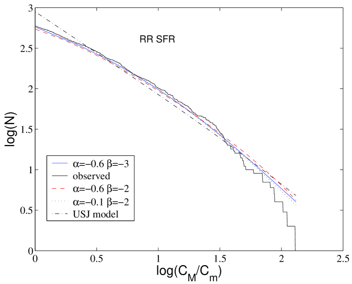
Figure 1: The predicted logN-log(P/P_lim) distribution for different values of $\alpha$ and $\beta$ with a RR-SFR vs. the observed logN-log(C_max/C_min) taken from the BATSE catalog. We also plot the predicted logN-log(P/P_lim) distribution in the USJ jet model, for which the inconsistency at the low peak flux range is apparent.

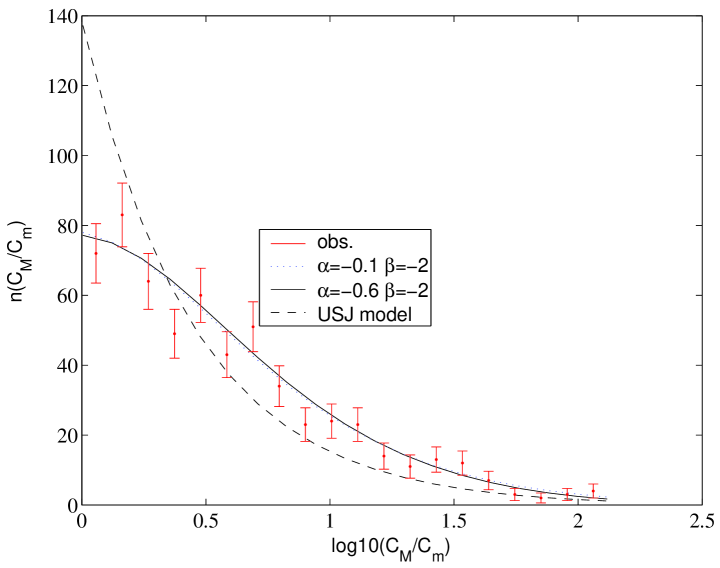
Figure 2: The predicted differential distribution, $n(P/P{\rm lim})$, for different values of $\alpha$ and $\beta$ with a RR-SFR vs. the observed n(C_max/C_min) taken from the BATSE catalog. We also plot the predicted differential distribution in the USJ jet model, for which the inconsistency at the low peak flux range is apparent.

From Figures 1 and 2 it is clear that the best set of values that reproduce the logN-log$(C_{\rm max}/C_{\rm min})$ distribution is $\alpha=-0.1$ and $\beta=-2$ and these will be the values used in the rest of our paper. Our results are slightly different from Schmidt’s mainly because we consider a different sample of GRBs and the quantity $P/P_{\rm lim}$ (which correspond to the observed $(C_{\rm max}/C_{\rm min})$) instead of the flux $P$ used by Schmidt (2001). In this way we take into account the fact that different bursts are detected with different flux thresholds.

So far we have used a parametric fit for the luminosity function. Within the USJ jet model, with $L\propto\theta^{-2}$ as forced by the energy-angle relation, we have a simple luminosity function: $\Phi_{sj}\propto L^{-2}$ (Perna et al. 2003). In Figures 1 and 2 we also compare the predicted logN-log$(P/P_{\rm lim})$ distribution that arises from this luminosity function with the RR-SFR with the observed logN-log$(C_{\rm max}/C_{\rm min})$ distribution. We find that within the USJ scenario the distribution is inconsistent with the data. The problem arises mostly for low peak fluxes. It is important to note, however, that our method of GRB selection does not introduce a bias against the inclusion of such low peak flux bursts. A “quasi-universal” jet (Zhang et al. 2003) obviously allows more freedom in fitting the data and may be consistent.

We can use now the luminosity function to derive the observed redshift distribution:

$$N(z)=\frac{R_{GRB}(z)}{1+z}\frac{dV(z)}{dz}\int_{L_{\rm min}(P_{\rm lim},z)}^{L_{\rm max}}\Phi_{o}(L)d\log L\ ,$$ (5)

where $L_{\rm min}(P_{\rm lim})$ is the luminosity corresponding to the minimum peak flux $P_{\rm lim}$ for a burst at redshift z and $L_{\rm max}=L^{*}\times\Delta_{2}=10\,L^{*}$. This minimal peak flux corresponds to the sensitivity of the gamma-ray burst detector used. We use, $P_{\rm lim}\sim 0.5-1$ ph cm${}^{-2}s^{-1}$, which is roughly the limiting flux for the GRBM on BeppoSAX (Guidorzi PhD thesis). We compare this distribution with the observed distribution of all the bursts with an available redshift: 32 bursts from http://www.mpe.mpg.de/ jcg/grbgen.html (excluding GRB980425 with $z=0.0085$). It is hard to quantify the selection effects that arise in the determination of the redshift. The problem is most severe in the range $1.3<z<2.5$ where visual spectroscopy (Hogg & Fruchter, 1999). Following Hogg & Fruchter (1999) we consider all the GRB with optical afterglow but without a measured redshift to be in this redshift range $1.3<z<2.5$. Using all the bursts in http://www.mpe.mpg.de/ jcg/grbgen.html we have a sample of 46 GRBs.

A comparison of the predicted cumulative redshift distribution with the observed one, (see Figure 3), reveals that with SF2 we obtain fewer bursts at low redshift than the observed ones. This happens even after taking into account the selection effects. In fact a Kolmogorov-Smirnoff test (KS) shows that the two distributions are only marginally compatible (5% level). The RR-SFR seems to reproduce better the redshift distribution, as the KS test shows that they are comparable at the level of 20%. Therefore we will focus on this distribution in the rest of the analysis.

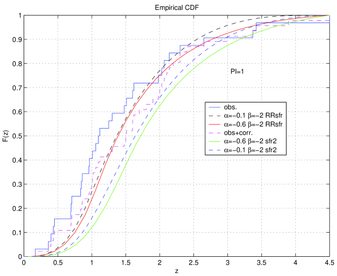
Figure 3: The predicted cumulative distributions of the GRBs redshift for the two SFR for $\alpha=-0.6$ (solid line) and our $\alpha=-0.1$ (dashed line). The histograms show the observed cumulative redshift distribution and a distribution where selection effects are taken into account assuming that all the GRB with no redshift but with optical afterglow lie in the range $1.3<z<2.5$.

3 Distribution of opening angles

We turn now to the peak luminosity - angle relation, which is analogous to the fluence - angle relation (Frail et al., 2001; Panaitescu & Kumar 2001). We consider a sample of 9 GRBs of the BATSE 4B catalog for which it has been possible to determine the redshift and the jet opening angle, $\theta$ (Bloom et al. 2003). In order to estimate the peak luminosity we need the peak fluxes. The advantage in taking only the BATSE GRBs is that we have all the peak fluxes estimated in the same way (averaged over the 1.024 sec BATSE trigger in the energy range 50-300 keV)

For all the bursts of this sample we estimate the peak luminosity along the jet of opening angle $\theta$ as:

$$L_{j}=f_{b}L.$$ (6)

In our analysis we consider the angles up to the maximum value implied by the observations ($\sim 0.7$ rad). Within this range of $\theta$ the beaming factor can be approximated as $f_{b}=(1-\cos\theta)\sim\theta^{2}/2$. In the upper panel of Figure 4 (left side) we show the distribution of $L_{j}$ obtained from this sample. Comparing this distribution with the isotropic one shown in the lower panel of the same figure (left side) we note that the peak luminosity, when corrected for beaming, is clustered around a value $L_{j}\sim 10^{49.5}$ erg/s. A similar result, shown in Figure 4 (right side), is obtained when we consider a larger sample, of 19 bursts with an angular estimate from 0.05 to 0.7 radians. Here there are larger uncertainties in the determination of the peak luminosity, as the bursts were detected by different detectors with different averaging time and different spectral resolution. We have extrapolated the GRB fluxes to the BATSE range 50-300 keV using the method described in Sethi & Bhargavi (2001) reelaborated for our spectrum. The redshifts and fluxes were taken from the table given in Van Putten & Regimbau (2003) who also find that the GRB peak luminosities and the beaming factors are correlated.

We find a correlation coefficient between $L$ and $1/f_{b}$ of $\sim 0.5$. The probability to obtain such a large value by chance, for uncorrelated $L$ and $1/f_{b}$, is smaller than 0.05. The regression line slope of log(L) vs log(1/f_b) is $\sim 0.8$.

The correlation is supported by a recent discovery of a relation between the observed peak energy, $E_{p}$, in the spectrum and L (Yonetoku et al. 2003). This together with the correlation between $E_{p}$ and the isotropic equivalent energy in $\gamma$-rays, $E_{\rm iso}$, (Amati et al. 2002 and Lamb, Donaghy & Graziani 2003) and with the Energy - angle relation (Frail et al., 2001; Panaitescu & Kumar 2001) imply $L_{j}=f_{b}L$. However, within the present sample there seem to be some spread in the value of $L_{j}$ as can be seen from Figure 4. To check the validity of our analysis we take this spread into account.

We first consider the case in which the distribution of $L_{j}$ is represented by a narrow-delta function and then discuss the effect of including the observed spread in $L_{j}$

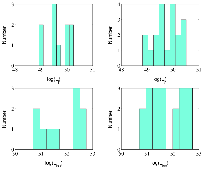
Figure 4: Left: the distribution of the isotropic peak luminosity (lower panel) and the distribution of the jet peak luminosity (upper panel) of 10 GRBs in the BATSE catalog with angle determination. Right: the distribution of the isotropic peak luminosity (lower panel) and the distribution of the jet peak luminosity (upper panel) of a large sample of 19 GRBs with angle determination.

Now if the jet angle and the peak luminosity are related we can derive the real distribution of the GRB jet opening angles. Let $P(\theta,L)$ be the distribution of number of bursts with opening angle $\theta$ and isotropic luminosity $L$. The observed distribution of number of bursts with opening angle $\theta$ in the small angles approximation can be written as:

$$P_{obs}(\theta) = \int f_{b}\,P(\theta,L)dL\sim\int\frac{\theta^{2}}{2}P(\theta,L)dL\qquad$$ (7)

$$\int_{0}^{z_{max}(\theta,P_{lim})}\frac{R_{GRB}(z)}{1+z}\frac{dV(z)}{dz}dz$$

Given the correlation between the GRB peak luminosity and the beaming factors we can assume that the condition $L(\theta^{2}/2)=L_{j}$, with $L_{j}$ roughly constant for all the GRBs, holds. Hence we have that $P(\theta,L)=\bar{P}(L)\delta(\theta-\sqrt{2L_{j}/L})$. Using the fact that $\bar{P}(L)=L/L_{j}\Phi(L)$ we obtain the intrinsic (corrected for beaming) angle distribution:

$$P(\theta)=\tilde{c}_{o}\left\{\begin{array}[]{ll}\theta^{*2\beta}\theta^{-2\beta-1}&\theta<\theta^{*}\\ \theta^{*2\alpha}\theta^{-2\alpha-1}&\theta>\theta^{*},\end{array}\right.$$ (8)

where $\tilde{c}_{o}$ is a normalization constant so that the integral over the angular distribution equals unity and $\theta^{*}\equiv\sqrt{2L_{j}/L^{*}}$ is the break angle of the $\theta$ distribution. $\theta^{*}\approx 0.12$rad with our canonical parameters. This equation should be compared with $P(\theta)\propto\sin\theta\sim\theta$ that is predicted by the USJ model. It is clear that the two distributions are inconsistent for large angles. A partial agreement is possible only for small angles with $\beta\approx-2$. The disagreement at large angles is just another indication of the fact that luminosity function implied by the USJ jet model is incompatible with the observed peak flux distribution at the low flux end (see Figure 1).

Substituting this relation in Eq.(7) and after some algebra we find the observed $\theta$ distribution:

$$P_{obs}(\theta) = {4c_{o}L_{j}\Phi(2L_{j}/\theta^{2})\over\theta^{3}}\qquad\qquad\qquad\qquad\qquad$$ (9)

$$\int_{0}^{z_{max}(\theta,P_{lim})}\frac{R_{GRB}(z)}{1+z}\frac{dV(z)}{dz}dz.$$

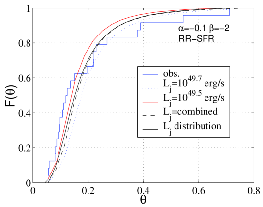
Figure 5: The predicted cumulative distributions of GRB opening angles for two different values of $L_{j}$ and for a combination of the two (reflecting the spread in the luminosity-angle relation) for RR-SFR. These results are compared to the curve obtained considering the observed distribution of $L_{j}$. The histograms show the observed cumulative opening angle distribution.

We compare the theoretical distribution with a sample of 24 GRBs with measured $\theta$ values (Blooom et al., 2003). We stress, again, that selection effects are hard to quantify especially for large and small opening angles. In Figure 5 we show the predicted cumulative $\theta$ distribution derived from our luminosity function with a RR-SFR and the observed one. We have chosen two values of $L_{j}$ as representative of the distributions given in Figure 4 (upper panel). We see that with these values of $L_{j}$ the opening angle distribution reproduces quite well the observed one.

We have repeated the analysis with a distribution of $\log_{10}(L_{j})$ with finite width, $\sim 0.4$, reflecting the spread in $L_{j}$ values seen in current data (Figure 4). The resulting $\theta$ distribution is similar to the one that arises from the combination of the two values of $L_{j}$ (black solid line in Figure 5).

Once we know the angular distribution we can turn to our final goal and estimate the true GRB rate. To do so we multiply the local observed rate, $\rho_{0}$ obtained in §2 by the correction factor that now can be estimated directly from the luminosity function given the relation between $f_{b}$ and $L$:

$$\langle f_{b}^{-1}\rangle=\frac{\int f_{b}^{-1}\Phi_{o}(L)d\log L}{\int\Phi_{o}(L)d\log L}\approx\frac{\int L/L_{j}\Phi_{o}(L)d\log L}{\int\Phi_{o}(L)d\log L}.$$ (10)

$\langle f_{b}^{-1}\rangle$ is the beaming factor averaged over the true, intrinsic, distribution of opening angles. We expect this average to be smaller that the value derived by Frail et al. (2001) due to the following reason: In the intrinsic luminosity distribution there are many bursts with a low luminosity and large opening angles. These bursts dominate the rate estimate and this should be factored in when calculating the average rate correction (Sari, 2003). Put differently, in the observed distribution, bursts with large $L$, i.e. large $f_{b}^{-1}$, are over-represented compared to the true distribution since they are observed to larger distances. In order to see this explicitly, we note that the $\langle f_{b}^{-1}\rangle$ can be derived directly from the observed distribution of GRB peak luminosities without deriving $\Phi(L)$, using the following argument. The total rate of GRBs (per unit $L$) in the observable universe is $d\dot{N}/d\log L=\rho_{0}(L/L_{j})\Phi(L)V_{U}$, where $V_{U}$ is the effective volume of the observable universe, $V_{U}=\int_{0}^{z_{m}}dz\,(dV/dz)R_{GRB}(z)/R_{GRB}(0)(1+z)$ ($z_{m}$ is the maximum redshift from which signals arrive at us by today). The observed rate is $d\dot{N}_{obs}/d\log L=\rho_{0}\Phi(L)V_{L}$, where $V_{L}$ is the volume out to $z_{L}$, the maximum redshift out to which bursts can be detected, $V_{L}=\int_{0}^{z(L)}dz\,(dV/dz)R_{GRB}(z)/R_{GRB}(0)(1+z)$. The beaming factor, defined in Eq. 10, can therefore be written as

$$\langle f_{b}^{-1}\rangle=\frac{\int dL\,\frac{d\dot{N}_{obs}}{dL}\frac{L}{L_{j}}\frac{V_{U}}{V_{L}}}{\int dL\,\frac{d\dot{N}_{obs}}{dL}\frac{V_{U}}{V_{L}}}.$$ (11)

Eq. 11 explicitly reflects the fact that in calculating the average beaming factor by which the observed local rate $\rho_{0}$ should be multiplied in order to obtain the true rate, $\langle f_{b}^{-1}\rangle$, the observed distribution of bursts should be weighted by $V_{U}/V_{L}$. Since $V_{U}/V_{L}$ is decreasing with $L$, a smaller weight is given to large $L$, i.e. to large $f_{b}^{-1}$, than in the observed distribution.

Using Eq. 10 with $L_{j}=10^{49.5}$ erg/s, we find $\langle f_{b}^{-1}\rangle\simeq 53$ for SF2 and $\langle f_{b}^{-1}\rangle\simeq 60$ for RR-SFR. These results do not change by inclusion of the dispersion in $L_{j}$. As expected, these values are lower than the value obtained by Frail et al. (2001), who derived $\langle f_{b}^{-1}\rangle$ by averaging without the $\propto V_{L}^{-1}$ weight. Using Eq. 11 with $L_{j}=10^{49.5}$ erg/s and RR-SFR we obtain $\langle f_{b}^{-1}\rangle\simeq 100$ for for the BATSE sample, and $\langle f_{b}^{-1}\rangle\simeq 50$ for the larger sample. Using Eq. 11 with $L_{j}$ determined for each burst from its estimated opening angle, we find $\langle f_{b}^{-1}\rangle\simeq 70$ for for the BATSE sample, and $\langle f_{b}^{-1}\rangle\simeq 55$ for the larger sample. The values obtained using these different choices are all within $\langle f_{b}^{-1}\rangle=75\pm 25$. This agreement reflects the fact that our derived $\Phi(L)$ gives a fair representation of the data. The range of values obtained reflects the range of uncertainty given current data.

We can also estimate the correction factor for the rate of GRB in the case of the USJ model in the following way: The total flux of GRBs per year (or per any other unit of time) is an observed quantity that can be obtained by summing over the observed distribution. In the USJ model the observed energy-angle relation implies: $E(\theta)=E_{0}/(\pi\theta^{2})$ for $\theta>\theta_{c}$ and $E(\theta)=E_{0}/(\pi\theta_{c}^{2})$ for $\theta<\theta_{c}$, where $\theta_{c}$ is the core angle of the jet. The total energy that a burst with a USJ emits is:

$$E_{\rm USJ} = 2[\int_{0}^{\theta_{c}}(E_{0}/\theta_{c}^{2})^{2}\theta d\theta+\int_{\theta_{c}}^{\theta_{\rm max}}E_{0}\theta^{-1}d\theta$$ (12)

$$= E_{0}[1+2\log(\theta_{\rm max}/\theta_{c})],$$

where $\theta_{max}$ is the maximal angle to which the jet extends.

This immediately implies that

$$N_{\rm uniform}/N_{\rm USJ}=[1+2\log(\theta_{\rm max}/\theta_{c})]$$ (13)

We don’t know for sure what are the upper and lower limits but the logarithmic dependance implies that the factor cannot be smaller than 2 or much larger than 5. This gives us the rate of uniform jets to be about factor of 4 below the number of “Uniform” jets. Put differently this suggest that the correction factor for the true rate of USJ compared to the rate of observed GRBs is a factor of $\sim 20\pm 10$.

4 Implications to Orphan Afterglows

The realization that gamma-ray bursts are beamed with rather narrow opening angles, while the following afterglow can be observed over a wider angular range, led to the search for orphan afterglows: afterglows that are not associated with observed prompt GRB emission. The observations of orphan afterglows would allow to estimate the opening angles and the true rate of GRBs (Rhoads 1997).

Nakar, Piran & Granot (2002) have estimated the total number of optical orphan afterglows given a limiting magnitude using the true rate of GRBs given by Frail et al. (2001). Nakar, Piran & Granot (2002) assumed, for simplicity, that all bursts have the same opening angle, denoted $\theta^{*}$. In their canonical model they assume that $\theta^{*}=0.1$rad while in the “optimistic” model they assume $\theta^{*}=0.05$rad. The smaller opening angle gives of course more orphan afterglows. This analysis have to be modified now using the new rate and the new correction factor that we have found. It is clear that the assumption of a fixed opening angle is not good enough and to obtain the rate of optical orphan afterglows one have to perform another weighted average over the observed $\theta$ distribution. This weight favors narrow jets which produce orphan afterglows over a wide solid angle and for which the rate correction is large. Overall (Nakar, 2003) one has to correct downwards by a factor of 1.6 the rates of the “canonical” model of Nakar, Piran & Granot (2002). The orphan afterglow rate obtained in the “optimistic” model are clearly an overestimate of the true rate, as this model assumed $\theta^{*}=0.05$ which is significantly lower than the average opening angle that we find here.

The situation is different for orphan radio afterglows, which are seen at large angles. We re-estimate the number of orphan radio afterglows associated to GRBs that should be detected in a flux-limited radio survey (Levinson et al. 2002). Levinson et al. have shown that the number of such radio afterglows detected over all sky at any given time above a threshold $f_{\nu,\rm min}$ at 1 GHz is

$$N_{R}\simeq 10\frac{\langle f_{b}^{-1}\rangle}{70}\left(\frac{\rho_{0}}{0.5\rm Gpc^{-3}yr^{-1}}\right)\left(\frac{f_{\nu,\rm min}}{5\rm mJy}\right)^{-3/2}$$

$$\varepsilon_{e,-0.5}^{3/2}\varepsilon_{B,-1}^{9/8}n_{-1}^{19/24}E_{51}^{11/6}.$$ (14)

Here, $E=10^{51}E_{51}$ ergs is the total fireball energy, assumed equal for all bursts following Frail et al. (2001) and Panaitescu & Kumar (2001), $n=10^{-1}n_{-1}{\rm cm^{-3}}$ is the number density of the ambient medium into which the blast wave expands, and $\varepsilon_{B}=10^{-1}\varepsilon_{B,-1}$ ($\varepsilon_{e}=10^{-0.5}\varepsilon_{e,-0.5}$) is the fraction of post shock thermal energy carried by magnetic field (electrons). For $f_{\nu,\rm min}\sim 5$ mJy, $N_{R}$ depends mainly on the local rate $\rho_{0}$ and only weakly on the redshift evolution of the GRB rate, since most of the detectable afterglows lie at low redshift $z\lesssim 0.2$ (Levinson et al. 2002).

Afterglow observations imply a universal value of $\varepsilon_{e}$ close to equipartition, $\varepsilon_{e,-0.5}\simeq 1$, based on the clustering of explosion energies Frail et al. (2001) and of X-ray afterglow luminosity (Freedman & Waxman 2001, Berger et al. 2003) The value of $\varepsilon_{B}$ is less well constrained by observations, since in most cases there is a degeneracy between $\varepsilon_{B}$ and $n$ in model predictions that can be tested by observations. The peak flux of a GRB afterglow seen by an observer lying along the jet axis is proportional to $E_{\rm iso}(n\varepsilon_{B})^{1/2}$, and for typical luminosity distance of $3\times 10^{28}$ cm it is $\approx 10(\varepsilon_{B}n/10^{-3}{\rm cm^{-3}})^{1/2}E_{\rm iso,54}$ mJy (Waxman 1997, Gruzinov & Waxman 1999, Wijers & Galama 1999). Here, $E_{\rm iso}=10^{54}E_{\rm iso,54}$ erg is the isotropic equivalent energy. Observed afterglow fluxes generally imply $\varepsilon_{B}n\geq 10^{-3}{\rm cm}^{-3}$ for $E_{\rm iso,54}\sim 0.1$, and values $\varepsilon_{B}n\sim 10^{-1}{\rm cm}^{-3}$ are obtained in several cases. We have therefore chosen the normalization $n_{-1}=\varepsilon_{B,-1}=1$ in Eq. (4).

Using our value for $\langle f_{b}^{-1}\rangle$, $\langle f_{b}^{-1}\rangle=70$ instead of $\langle f_{b}^{-1}\rangle=500$ given in Frail et al. (2001), reduces the number of expected radio afterglows by a factor of $\sim 7$. However, the number of afterglows expected to be detected by all sky $\sim 1$ mJy radio surveys is still large, exceeding several tens.

It should be pointed out that the lower limit on the beaming factor inferred from the analysis of Levinson et al. (2002) is unaffected by our modified value of $\langle f_{b}^{-1}\rangle$. Assuming a fixed value of $f_{b}$ and expressing $N_{R}$ in terms of the isotropic equivalent GRB energy, $E_{\rm iso.}=10^{54}E_{\rm iso.,54}$ ergs, we have

$$N_{R}\simeq 10^{4.5}f_{b}^{5/6}\left(\frac{\rho_{0}}{0.5\rm Gpc^{-3}yr^{-1}}\right)\varepsilon_{e,-0.5}^{3/2}$$

$$\varepsilon_{B,-1}^{9/8}n_{-1}^{19/24}E_{\rm iso.,54}^{11/6}.$$ (15)

Formally, the average value of $E_{\rm iso.}^{11/6}$ should appear in this equation. We have chosen $<E_{\rm iso.}^{11/6}>^{6/11}=10^{54}$ erg as a representative value. The upper limit on the number of afterglows derived in Levinson et al. (2002) implies a lower limit on the beaming factor, $f_{b}^{-1}>40$ for the parameter choice in Eq. (15), indicating that radio surveys may indeed put relevant constraints on the beaming factor.

5 Conclusion

In this work a combined L-$\theta$ distribution function of GRBs is derived, $\Phi(L,\theta)$, for the uniform jet model. To this aim we have rederived (following Schmidt, 1999) the luminosity function, $\Phi(L)$ by fitting the peak flux distribution and used the relation $L\times\theta^{2}\sim$ const implied by the observation on the sample considered by Bloom et al. (2003). We have compared our results with those obtained in the framework of USJ jet model (Perna et al. 2003) showing that the luminosity function implied by this model leads to a peak flux distribution some what inconsistent with the observed one.

The luminosity function that best fits the observed peak flux distribution is characterized by two power laws with slopes $\alpha=-0.1$ and $\beta=-2$ and isotropic-equivalent break luminosity $L^{*}\sim 7.1\times 10^{51}$ erg/s for a SF2 or $L^{*}\sim 4.4\times 10^{51}$ erg/s for a RR-SFR. Repeating the Schmidt analysis we have found the observed local rate of long GRBs $\rho_{0}\sim 0.10$ Gpc^-3yr^-1 and $\rho_{0}\sim 0.44$ Gpc^-3yr^-1 for the two SFR respectively. We have also shown that with these luminosity functions we find a reasonable agreement with the observed redshift distribution for a RR-SFR, while a SF2 predicts too few bursts at low redshift. Nevertheless since the redshift sample is strongly affected by selection effects that are hard to estimate the possibility that GRBs follow the SF2 cannot be ruled out by this analysis.

Using the sample of Bloom et al. (2003) we have shown that the energy-angle relation (Frail et al., 2001; Panaitescu & Kumar 2001) applies also to the peak luminosity and that there is a clustering of the true peak luminosity around $\sim 3.2\times 10^{49}$ erg/s. However the distribution is not a narrow delta-function. This implies that a luminosity function determines a $\theta$ distribution as $L$ is related to $\theta$. This is true even when the spread in $L_{j}$ observed in the current data is taken into account. One important result of our work is that the resulting angular distribution found under this assumption is consistent with the observation.

We have re-calculated the correction to the rate of GRBs due to beaming using a weighted average of the predicted angular distribution instead of a simple average over the “true” angular distribution as done by Frail et al. (2001) and by van Putten & Regimbau (2003). We find a correction factor $75\pm 25$ (see the end of § 3). This is significantly smaller than the commonly used correction factor, $\sim 500$, estimated by Frail et al. (2001) or $\sim 475$ estimated by van Putten & Regimbau (2003). . This correction should also influence the estimated rates of both optical (Nakar, Piran & Granot, 2002) and radio (Levinson et al., 2002) orphan afterglows (see § 4).

The research was supported by the RTN “GRBs - Enigma and a Tool” and by an ISF grant for a Israeli Center for High Energy Astrophysics. DG thanks the Weizmann institute for the pleasant hospitality acknowledges the NSF grant AST-0307502 for financial support. We thank Marteen Schmidt, Ehud Nakar and Cristiano Guidorzi for helpful discussions.

References

- (1) Amati, L. et al. 2002, A&A, 390, 81.
- Berger et al. (2003) Berger, E., Kulkarni, & S. R., Frail, D. A. 2003, ApJ590, 379
- Bloom et al. (2003) Bloom, J., Frail, D. A. & Kulkarni, S.R., 2003, ApJ 594, 674.
- Cohen & Piran (1995) Cohen, E. & Piran, T., 1995, ApJL, 444, L25.
- Fenimore & Ramirez-Ruiz (2000) Fenimore, E. & Ramirez-Ruiz, E. 2000, astro-ph/0004176.
- Fenimore & Bloom (1995) Fenimore, E. E., and J. S. Bloom,1995, ApJ 453,25.
- Frail et al. (2001) Frail, D. A. et al., 2001, ApJ 562, L55.
- Freedman & Waxman (2001) Freedman, D.L., & Waxman, E. 2001, ApJ, 547, 922.
- Gruzinov & Waxman (1999) Gruzinov, A. & Waxman, E. 1999, ApJ, 511, 852
- Guidorzi (2002) Guidorzi, C. 2002, PhD Thesis, University of Ferrara.
- (11) Hogg, D. W. & Fruchter, A. S., 1999, ApJ 520, 54.
- Horack & Hakkila (1997) Horack, J. M., and J. Hakkila, 1997, ApJ 479, 371.
- (13) Kouveliotou, C. et al., 1993, ApJ 431, 101.
- (14) Lamb, D. Q., Donaghy, T. Q., Graziani, C., 2004, New Astronomy Reviews 48,459.
- Levinson et al. (2002) Levinson, A. et al. 2002, ApJ 576, 923.
- Loredo & Wasserman (1995) Loredo, T. J., and I. M. Wasserman, 1995, ApJs 96, 261.
- Loredo & Wasserman (1998) Loredo, T. J., and I. M. Wasserman, 1998, ApJ 502, 75.
- (18) Paciesas, W. et al., 1999, ApJS 122, 456.
- (19) Nakar, E., Piran, T. & Granot, J., 2002, ApJ 579, 699.
- (20) Nakar, E., 2003, private communication.
- Norris et al. (2000) Norris, J. P., Marani, G.F. & Bonnell, J. T., 2000, ApJ 534, 248.
- Panaitescu & Kumar (2001) Panaitescu, A. & Kumar, P., 2001, ApJ 561, L167.
- Perna et al. (2003) Perna, R., Sari, R., Frail D., 2003, ApJ, 594, 379.
- Piran (1992) Piran, T., 1992, ApJL, 389, L45.
- Piran (1999) Piran, T., 1999, Physics Reports, 314, 575.
- Porciani and Madau (2001) Porciani, C., and P. Madau, 2001, ApJ 548, 522.
- Rhoads (1997) Rhoads, J. E., 1997, ApJ 487 L1.
- Rossi et al. (2002) Rossi, E., Lazzati, D. & Rees, M. J., 2002, MNRAS 332, 945.
- Rowan-Robinson (1999) Rowan-Robinson, M. 1999, Ap&SS, 266, 291.
- Sari et al (1999) Sari, R., Piran, T. & Halpern, J. P., 1999, ApJ 519, L17.
- (31) Sari, R., 2003, talk given at the Santorini meeting, August, 2003.
- Schmidt (1999) Schmidt, M., 1999, ApJ 523, L117.
- Schmidt (2001) Schmidt, M., 2001, ApJ 552, 36.
- Schmidt (2003) Schmidt, M., 2003, contribution for Rome 2002, GRB workshop.
- Sethi & Bhargavi (2001) Sethi, S., and S. G. Bhargavi, 2001, A&A376, 10.
- Van Putten & Regimbau (2003) Van Putten, M. & Regimbau, T., 2003, ApJ 593, L15.
- (37) Waxman, E. 1997b, ApJ, 489, L33
- (38) Waxman, E., Kulkarni, S. R. & Frail, D. A. 1998, ApJ 497, 288.
- Wijers & Galama (1999) Wijers, R. A. M. J. & Galama, T. J., 1999, ApJ, 523, 177
- (40) Yonetoku, D. et al. astro-ph/0309217
- (41) Zhang, B., Dai, X., Lloyd-Ronning, N. M. & Mészáros P., astro-ph/0311190.