Ultra High Energy Cosmic Rays

Abstract

Cosmic rays with energies above $10^{18}$ eV are currently of considerable interest in astrophysics and are to be further studied in a number of projects which are either currently under construction or the subject of well-developed proposals. This paper aims to discuss some of the physics of such particles in terms of current knowledge and information from particle astrophysics at other energies.

Department of Physics, The University of Adelaide
Adelaide, Australia 5005
¹rprother@physics.adelaide.edu.au, ²rclay@physics.adelaide.edu.au

Keywords: cosmic rays, acceleration of particles, magnetic fields, dark matter, radiation mechanisms: nonthermal, diffuse radiation

1 Introduction

Cosmic rays (CR) are the non-photon particles with which we learn about astrophysics. Their composition ranges over the known nuclei (and antiprotons) to electrons (and positrons) and neutrinos of all flavours, and (perhaps) to exotic particles as yet unobserved in accelerator physics. Cosmic ray studies are complementary to photon astrophysics since many astrophysical photons are produced in processes, such as synchrotron emission, which involve charged cosmic ray particles. In this review we concentrate on the highest energy cosmic rays, which are unaffected by heliospheric modulation, but are strongly affected by propagation effects through our galaxy. In the case of an extragalacic origin for the highest energy cosmic rays, their propagation through intergalactic photon and magnetic fields will have a profound influence on what we observe.

Radio astronomical studies probe cosmic rays at their sources and we are led to associate cosmic ray acceleration with energetic radio objects, pulsars, supernovae, AGNs etc. The next generation of large radio projects (LOFAR, SKA etc.) will certainly add considerably to our understanding of cosmic ray sources, and may even offer opportunities to develop new detection techniques through the radio-frequency fields of the air showers of cosmic rays arriving at Earth (e.g. Falcke and Gorham 2003).

The radio emission is dominated by cosmic ray electrons which rapidly lose energy in the emission processes. The more massive nuclei do not have a clear radio signature but propagate with little energy loss and are readily observed at Earth. They are believed to fill (at least) the volume of our galaxy. However, being charged particles, their paths are dictated by astrophysical magnetic fields and only at the highest energies do we expect magnetic deflections to be sufficiently small for directional astrophysics to be possible.

At modest energies (up to about $10^{14}$eV), cosmic rays are sufficiently plentiful that balloon experiments can have enough collecting area to directly study properties of the beam. Indeed, even satellite experiments extend up to 2 TeV/amu (for the CRN experiment on Spacelab 2, Müller et al 1991) which for iron is about $10^{14}$eV per nucleus. At higher energies, we depend on techniques which investigate the cascades of particles (extensive air showers) resulting from the impact of cosmic ray particles on our atmospheric gas. Since a single cosmic ray particle can produce millions (or billions) of secondary particles in this way, and those particles scatter in the atmosphere to hundreds of metres from the original cosmic ray trajectory, such studies offer uniquely efficient opportunities for studying fluxes down to levels of primary CR particles per square kilometre per century.

The cosmic ray cascades may be directly detected with groups of spaced large-area radiation detectors on the ground (ground arrays) or indirectly through collecting (with large telescopes) the photons which they produce, fluorescence light from atmospheric nitrogen or Cerenkov emission from the bulk atmospheric gas. In the future, such light collectors may well be satellite-based.

The Ultra High Energy cosmic rays (UHE CR) which are the focus of this review are currently of particular interest. Spectral data at energies above 1 EeV ($10^{18}$eV) and directional results, notably from the AGASA project, are very suggestive of fascinating, unexpected physics (Hayashida et al. 1999). Furthermore, this field of research is experimentally challenging and there is controversy in discrepancies between experimental data from experiments currently operational or recently discontinued. A new era in the field is beginning with the commissioning of the Pierre Auger Observatory (Auger Collaboration 2001) which comprises a pair of 3000 km² arrays (one under construction in Mendoza Province, Argentina, and one planned for Utah, U.S.A) employing both particle and optical detectors, followed by large-scale Japanese projects, and possibly the space-based Extreme Universe Space Observatory project (EUSO is a Europe/Japan/US collaboration currently under Phase A study as an ESA mission with the goal of a three-year mission on the ISS starting in 2009, see http://www.euso-mission.org/).

At the present time, our ideas concerning cosmic rays at these highest energies are predominantly based on the idea that such particles are likely to be of extragalactic origin. Their sources are presumed to be found in some extreme astrophysical environment such as the most energetic radio or gamma-ray sources. We have been forced to these ideas by our failure to identify any models for galactic objects capable of accelerating particles to within one thousandth of the required energies, and also by the failure of our galactic source models to reproduce the directional isotropy of the observed beam. Nonetheless, extragalactic scenarios have their own problems. The intergalactic magnetic field has largely unknown properties. It could be strong enough, with a structure which makes it impenetrable to particles from nearby clusters of galaxies in realistic periods of time. Also, intracluster magnetic fields may limit the ability of particles even to leave galactic clusters.

This paper begins by presenting a brief overview of the observed properties (energy spectrum, arrival directions, and composition) of the cosmic ray beam. There follows a physical discussion of the cosmic ray acceleration process and resulting limits to the maximum achievable energies. Energy losses in the following propagation through astrophysical fields are fundamental in determining the observed beam properties and these are then discussed. It is possible that the origin of the highest energy cosmic rays lies in exotic particles and that field of research is introduced. Whatever the sources of these particles may be, their observed directional properties will be closely linked with the properties of the intervening magnetic fields. A discussion of this key factor completes our review. For an earlier review see Nagano and Watson (2000).

1.1 The Detection of Ultra High Energy Cosmic Rays

Cosmic ray observatories record the arrival directions and distribution of energies of incident particles. They also attempt to measure a remaining parameter, which is the mass composition of the primary cosmic ray particle. It is in the latter respect that cosmic ray studies differ from others in astrophysics. The mass composition is a key parameter in our astrophysical understanding since the charge on the particle (closely related to mass, for a nucleus), with the momentum (or energy) determines the propagation path of the particle.

At the highest energies, the cosmic ray flux is extremely low and the particle recording must be through processes which enable detection to be achieved at large distances from the path of the primary cosmic ray. In practice, this involves making use of the particle cascade which results from the interaction of the primary cosmic ray particle with our atmosphere.

That cascade is initiated by a primary cosmic ray particle when its first atmospheric interaction occurs. A cascade of secondary particles is then fed by degrading energy from the primary particle as it repeatedly interacts in its atmospheric passage. Those secondary particles cause energy to be deposited into the atmospheric gas, with some remaining energy reaching the ground. The cosmic ray detection process then consists in either a measurement of the passage of the energy as it is carried by particles through the atmosphere (through any emitted Cerenkov light or by any induced nitrogen fluorescence light) or in direct detections in radiation detectors of remaining particles which reach the ground.

The arrival direction of the primary particle is deduced from the direction of the path of the atmospheric cascade and characteristically has a resolution of a fraction of a degree. The primary particle energy is deduced by attempting to make sufficient measurements on the cascade such that a calorimetric accounting (to a few tens of percent) can be made of the various energy sinks. This is most directly done through nitrogen fluorescence studies, but the signal is weak and the technique works best at the highest energies. Mass composition measurements are the most difficult, and cannot be made on an individual cascade basis. They depend on statistical studies of the cascade developments as a function of energy. Crudely speaking, massive nuclei have a large cross section and interact early. Their cascades also degrade in energy relatively rapidly. As a result, early developing cascades are signatures of ’heavy’ primaries and late developing cascades are indicative of ’light’ (probably proton) primaries. Massive amounts of cascade modelling puts flesh on these arguments.

Nitrogen fluorescence studies were pioneered by the Fly’s Eye experiment (Baltrusaitis et al. 1985) and its successor, the High Resolution Fly’s Eye (HiRes). Many ground detector arrays have been used. The largest one in fully developed use is the AGASA (Hayashida et al. 1999) experiment in Japan. Both of the HiRes and AGASA experiments are sufficiently large to probe energies in excess of $10^{20}$eV. The next of these huge experiments will use both techniques. The Pierre Auger Observatory (Auger Collaboration 2001) is designed to operate above $10^{19}$eV. It will have a 3000 square kilometre collecting area instrumented with 1600 large-area particle detectors and will also have twenty-four 4 m diameter Schmidt optical telescopes for fluorescence detection.

1.2 The Cosmic Ray Energy Spectrum

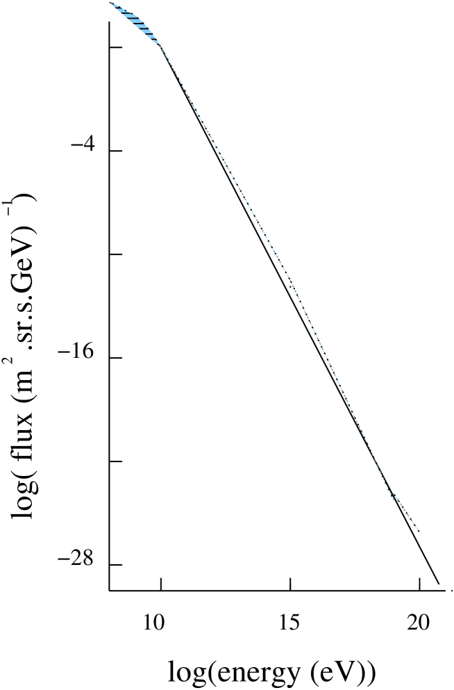
Figure 1: The cosmic ray energy spectrum (dotted) as measured from the Earth (after Bhattacharjee and Sigl 2000).

The cosmic ray energy spectrum is shown in Fig. 1. It is remarkable both in its range of energies and in its range of fluxes. It covers over ten decades of energy and thirty decades of flux in a form close to a power law with an index of about -2.7. Deviations from that power law are relatively small but are generally regarded as physically significant. There is a steepening at about $10^{16}$eV, known as the knee, and a flattening at about $10^{18}$eV known as the ankle (e.g. Abu-Zayyad et al. 2001). The knee is often argued to be associated with an energy limit of acceleration from supernova remnant sources, although it may well be related to a loss of ability for our galactic magnetic fields to retain (and build up internally) the cosmic ray flux (e.g. Clay 2002). The ankle is usually associated with the onset of a dominant, flatter, extra-galactic cosmic ray spectrum. It is important to note that, in this model, our galaxy produces particles with energies up to those of the ankle of the spectrum. That is already above 1 EeV$\equiv$$10^{18}$eV, and is well above energies which are easily accessible for any present galactic acceleration models.

A key region of the spectrum is its very highest energies. The flux here is so low that the low event statistics in our observations to date leave us uncertain of the spectral structure above the key energy of $6\times 10^{19}$eV. Here there is a predicted spectral downturn, the Greisen-Zatsepin-Kuzmin (GZK) cut-off (Greisen 1966, Zatsepin and Kuzmin 1966) for particles which have travelled more than a few tens of Mpc, due to interactions with the 2.7K cosmic microwave background radiation (CMBR). However, several experiments have reported CR events with energies above $10^{20}$ eV (Takeda et al. 2003) with the highest energy event having 300 EeV (Bird et al. 1995). Very recent data from the two largest aperture high energy cosmic ray detectors are contradictory: AGASA (Takeda et al. 2003) observes no GZK cut-off while HiRes (Abu-Zayyad et al. 2002) observes a cut-off consistent with the expected GZK cut-off. A systematic over-estimation of energy of about 25% by AGASA or under-estimation of energy of about 25% by HiRes could account the discrepancy (Abu-Zayyad et al. 2002), but the continuation of the UHECR spectrum to energies well above $10^{20}$ eV is now far from certain. Future measurements with Auger (Auger Collaboration 2001) should resolve this question. If the spectrum does extend well beyond $10^{20}$ eV, determining the origin of these particles could have important implications for astrophysics, cosmology and particle physics.

1.3 Arrival Directions

A key observation in cosmic ray astrophysics is the directional distribution of the particles. That distribution will depend on any galactic magnetic fields and hence will be energy (rigidity) dependent. However, with very limited exceptions, which are not individually statistically significant, there is no observed deviation from isotropy above the knee of the energy spectrum, and any anisotropies at lower energies are themselves very small (Smith and Clay 1997, Clay, McDonough and Smith 1997). Recently, the AGASA experiment (Hayashida et al. 1999) found a non-uniform distribution of arrival directions, suggestive of a source direction, in the energy range $10^{18.0}$eV to $10^{18.4}$eV. That observation is potentially very important, particularly as there is supporting evidence in data from the SUGAR array (Bellido et al. 2001). However, neither of those observations on their own is clearly statistically significant. Still, those data are regarded by many as the possible beginning of a new era in cosmic ray astrophysics in which we can begin directional cosmic ray astronomy. The possibility of having a source to observe may indeed open up new frontiers.

1.4 Composition of the UHECR

The highest energy cosmic rays show no major differences in their air shower characteristics to cosmic rays at lower energies. One would therefore expect the highest energy cosmic rays to be protons particularly if, as is most likely, they are extragalactic in origin. However, it is still possible that they are not single nucleons. Obvious candidates are heavier nuclei (e.g. Fe), $\gamma$-rays and neutrinos. Surprisingly, it is even more difficult to propagate nuclei than protons, because of the additional photonuclear disintegration (Tkaczyk et al. 1975, Puget et al. 1976, Karakula and Tkaczyk 1993, Elbert and Sommers 1995, Anchordoqui et al. 1997, Stecker and Salamon 1999). The possibility that the 300 EeV Fly’s Eye event is a $\gamma$-ray has been discussed (Halzen et al. 1995) and, although not completely ruled out, the air shower development profile seems inconsistent with a $\gamma$-ray primary. Weakly interacting particles such as neutrinos will have no difficulty in propagating over extragalactic distances, of course. This possibility has been considered, and generally discounted (Halzen et al. 1995, Elbert and Sommers 1995), mainly because of the relative unlikelihood of a neutrino interacting in the atmosphere, and the resulting great increase in the luminosity required of cosmic sources.

1.5 Cosmic Ray Sources

Figure 2 is a well known diagram first produced by Hillas (1984). It reminds us that acceleration, associated with magnetic structures, requires the field and its dimensions to be sufficient to contain the accelerating particle through the acceleration process. The lines simply give the magnetic field vs. gyroradii $r_{g}$ for protons (solid) and iron nuclei (dashed), and this gives the minimum size for scattering centres moving at at speeds $\sim c$. More realistically, for scattering centres moving at speeds $v_{\rm scat}<c$ the size would need to be a factor $c/v_{\rm scat}$ larger. This puts a limit on the product of the source field and its physical dimensions. Strong fields with large-scale structure are attractive for acceleration to the highest energies. The acceleration is thought to be likely to be associated with astrophysical shocks.

Figure 2: Proposed sites for cosmic ray acceleration related to their likely dimensions and magnetic field strength for scattering centres moving with $v_{\rm scat}\sim c$ (after Hillas 1984). The lines represent plausible limits for $10^{20}$eV cosmic ray containment in the sources (solid line – protons, dashed line – iron nuclei) for scattering centres moving at at speeds $\sim c$. For scattering centres moving at speeds $v_{\rm scat}<c$ the size would need to be a factor $c/v_{\rm scat}$ larger.

One of the very few plausible acceleration sites may be associated with the radio lobes of powerful radio galaxies, either in the hot spots (Rachen and Biermann 1993) or possibly the cocoon or jet (Norman et al. 1995). One-shot processes such as magnetic reconnection (e.g. in jets or accretion disks) comprise another possible class of sources (Haswell et al. 1992, Sorrell 1987).

Acceleration at the termination shock of the galactic wind from our Galaxy has also been suggested by Jokipii and Morfill (1985), but due to the lack of any statistically significant anisotropy associated with the Galaxy it is unlikely to be the explanation. However, a re-evaluation of the world data set of cosmic rays has shown that there is a correlation of the arrival directions of cosmic rays above 40 EeV with the supergalactic plane (Stanev et al. 1995), lending support to an extragalactic origin above this energy, and in particular to models where “local” sources ($<100$ Mpc) would appear to cluster near the supergalactic plane. Such a correlation would also be consistent with a Gamma Ray Burst (GRB) origin as two type Ic hypernovae (supernovae with broad absorption features indicating high velocity ejected material and a rather large explosion energy) have now been identified with GRB (SN 2003dh/GRB 030329 Kawabata et al. 2003; SN 1998bw/GRB980425 Galama et al. 1998). The expanding fireball may have ultrarelativistic components (e.g. $\Gamma\sim 300$) and this may lead to production of UHECR through relativistic shock acceleration (Vietri 1995) or some other process (see e.g. Dermer 2002 for a discussion and references to earlier work).

Because of the resulting flat spectrum of particles (including gamma-rays and protons) extending up to GUT (grand unified theory) scale energies, topological defect models have been invoked to try to explain the UHE CR. Propagation of the spectra of all particle species over cosmological distances is necessary to predict the cosmic ray and gamma-ray spectra expected at Earth. Propagation over cosmological distances to Earth (as would be the case in some topological defect origin models) results in potentially observable gamma-ray fluxes at GeV energies in addition to cosmic rays. Massive relic particles on the other hand, would cluster in galaxy halos, including that of our Galaxy, and may give rise to anisotropic cosmic ray signals at ultra high energies.

The suggestion that neutron stars might accelerate cosmic rays followed soon after the discovery of pulsars (see, e.g. Gold 1975 and references therein). Voltages up to $\sim 10^{12}$–$10^{15}$V (depending on pulsar period and magnetic field) are expected in a pulsar’s magnetosphere. These could accelerate nuclei with a resulting flat spectrum extending up to $\sim$10¹⁶ eV, and could possibly explain the knee in the cosmic ray spectrum (e.g. Bednarek & Protheroe 2002). The pulsar wind shock has been proposed as an acceleration site (e.g., Berezhko 1994, Bell and Lucek 1996) and might in principle accelerate particles to $10^{15}$–$10^{19}$eV. Blasi et al. (2000) suggest that the UHE CR events are due to iron nuclei accelerated from young strongly magnetized neutron stars through relativistic MHD winds of neutron stars whose initial spin periods are shorter than $\sim 10$ ms. More recently, the acceleration to ultra-high energies has been discussed in the context of fast re-connection in millisecond pulsars, but it appears that to reach $\sim 10^{20}$ eV magnetic fields $\sim 10^{12}$–$10^{15}$ G, and special geometries are required (de Gouveia Dal Pino and Lazarian, 2001). In our opinion, while neutron stars may contribute to the observed cosmic ray spectrum it seems unlikely that they are responsible for the UHE CR, with the possible exception of transient shocks in pulsar winds of neutron stars formed during a hypernova explosion (i.e. a GRB as already discussed).

We shall delay a more detailed discussion of radio galaxies, active galactic nuclei and topological defects as sources of the UHE CR, and discuss next diffusive shock acceleration and cosmic ray propagation.

2 Diffusive Shock Acceleration

For stochastic particle acceleration by electric fields induced by the motion of magnetic fields $B$, the rate of energy gain by relativistic particles of charge $Ze$ can be written (in SI units)

$$\left.{dE\over dt}\right|_{\rm acc}=\xi(E)Zec^{2}B$$ (1)

where $\xi(E)<1$ and depends on the acceleration mechanism. Below is a simple heuristic treatment of Fermi acceleration based on those given by Gaisser (1990) and Protheroe (2000). We shall start with 2nd order Fermi acceleration (Fermi’s original theory) and describe how this can be modified in the context of astrophysical shocks into the more efficient 1st order Fermi mechanism known as diffusive shock acceleration. More detailed and rigorous treatments are given in several review articles (Drury 1983a, Blandford and Eichler 1987, Berezhko and Krymsky 1988). See the review by Jones and Ellison (1991) on the plasma physics of shock acceleration which also includes a brief historical review and refers to early work.

2.1 Fermi’s Original Theory

Gas clouds in the interstellar medium have random velocities of $\sim 15$ km/s superimposed on their regular motion around the galaxy. Cosmic rays gain energy on average when scattering off these magnetized clouds. A cosmic ray enters a cloud and scatters off irregularities in the magnetic field which is tied to the partly ionized cloud.

Figure 3: Interaction of cosmic ray of energy $E_{1}$ with “cloud” moving with speed $V$

In the frame of the cloud: (a) there is no change in energy because the scattering is collisionless, and so there is elastic scattering between the cosmic ray and the cloud as a whole which is much more massive than the cosmic ray; (b) the cosmic ray’s direction is randomized by the scattering and it emerges from the cloud in a random direction.

Consider an ultra-relativistic cosmic ray entering a cloud with energy $E_{1}$ and momentum $p_{1}\approx E_{1}/c$ travelling in a direction making angle $\theta_{1}$ with the cloud’s direction. After scattering inside the cloud, it emerges with energy $E_{2}$ and momentum $p_{2}\approx E_{2}/c$ at angle $\theta_{2}$ to the cloud’s direction (Fig. 3). The energy change is obtained by applying the Lorentz transformations between the laboratory frame (unprimed) and the cloud frame (primed). Transforming to the cloud frame:

$$E_{1}^{\prime}=\gamma E_{1}(1-\beta\cos\theta_{1})$$ (2)

where $\beta=V/c$ and $\gamma=1/\sqrt{1-\beta^{2}}$.

Transforming to the laboratory frame:

$$E_{2}=\gamma E_{2}^{\prime}(1+\beta\cos\theta_{2}^{\prime}).$$ (3)

The scattering is collisionless, being with the magnetic field. Since the magnetic field is tied to the cloud, and the cloud is very massive, in the cloud’s rest frame there is no change in energy, $E_{2}^{\prime}=E_{1}^{\prime}$, and hence we obtain the fractional change in LAB-frame energy $(E_{2}-E_{1})/E_{1}$,

$${\Delta E\over E}={1-\beta\cos\theta_{1}+\beta\cos\theta_{2}^{\prime}-\beta^{2}\cos\theta_{1}\cos\theta_{2}^{\prime}\over 1-\beta^{2}}-1.$$ (4)

We need to obtain average values of $\cos\theta_{1}$ and $\cos\theta_{2}^{\prime}$. Inside the cloud, the cosmic ray scatters off magnetic irregularities many times so that its direction is randomized,

$$\langle\cos\theta_{2}^{\prime}\rangle=0.$$ (5)

The average value of cos$\theta_{1}$ depends on the rate at which cosmic rays collide with clouds at different angles. The rate of collision is proportional to the relative velocity between the cloud and the particle so that the probability per unit solid angle of having a collision at angle $\theta_{1}$ is proportional to $(v-V\cos\theta_{1})$. Hence, for ultrarelativistic particles ($v=c$)

$${dP\over d\Omega_{1}}\propto(1-\beta\cos\theta_{1}),$$ (6)

and we obtain

$$\langle\cos\theta_{1}\rangle=\int\cos\theta_{1}{dP\over d\Omega_{1}}d\Omega_{1}/\int{dP\over d\Omega_{1}}d\Omega_{1}=-{\beta\over 3},$$ (7)

giving

$${\langle\Delta E\rangle\over E}={1+\beta^{2}/3\over 1-\beta^{2}}-1\simeq{4\over 3}\beta^{2}$$ (8)

if $\beta\ll 1$.

We see that $\langle\Delta E\rangle/E\propto\beta^{2}$ is positive (energy gain), but is 2nd order in $\beta$ and if $\beta\ll 1$ the average energy gain per cloud collision is very small. This is because there are almost as many overtaking collisions (energy loss) as there are head-on collisions (energy gain). The acceleration rate is

$$r_{\rm acc}(E)\equiv{1\over E}\left.{dE\over dt}\right|_{\rm acc}={\langle\Delta E\rangle\over E}r_{\rm coll}\simeq{4\over 3}\left({V\over c}\right)^{2}r_{\rm coll}$$ (9)

where $r_{\rm coll}$ is the rate of collision of the cosmic ray with the cloud. 2nd order Fermi acceleration is one example of stochastic acceleration. Another example involves the average energy gain that arises in resonant interactions of cosmic rays with Alfvén waves. In this case, the acceleration rate would be

$$r_{\rm acc}(E)\propto\left({v_{A}\over v}\right)^{2}r_{\rm coll}$$ (10)

where $v_{A}$ is the Alfvén velocity and $r_{\rm coll}$ is now the rate of collision of the cosmic ray (speed $v$) with the Alfvén waves (see e.g. Jones 1994).

2.2 1st Order Fermi Acceleration at Astrophysical Shocks

Fermi’s original theory was modified in the 1970’s (Axford, Lear and Skadron 1977, Krymsky 1977, Bell 1978, Blandford and Ostriker 1978) to describe more efficient acceleration (1st order in $\beta$) taking place at supernova shocks but is generally applicable to strong shocks in other astrophysical contexts. Our discussion of shock acceleration will be of necessity brief, and omit a number of subtleties.

Here, for simplicity, we adopt the test particle approach (neglecting effects of cosmic ray pressure on the shock profile), adopt a plane geometry and consider only non-relativistic shocks. Nevertheless, the basic concepts will be described in sufficient detail that we can consider acceleration and interactions of the highest energy cosmic rays, and to what energies they can be accelerated. We consider the classic example of a SN shock. During a supernova explosion several solar masses of material are ejected at a speed of $\sim 10^{4}$ km/s which is much faster than the speed of sound in the interstellar medium (ISM) which is $\sim$ 10 km/s. A strong shock wave propagates radially out (speed $V_{S}$) as the ISM and its associated magnetic field piles up in front of the supernova ejecta which moves at speed $V_{P}$ (see Fig. 4a). As seen in the frame of the shock (see Fig. 4b) gas flows from upstream into the shock with speed $u_{1}=V_{S}$ and density $\rho_{1}$, and flows out of the shock downstream with speed $u_{2}=(V_{S}-V_{P})$ and density $\rho_{2}$. The velocity of the shock, $V_{S}$, depends on the velocity of the piston (ejecta), $V_{P}$, and on the ratio of specific heats, $\gamma$. The compression ratio for a strong non-relativistic shock is given by

$$R={\rho_{2}\over\rho_{1}}={u_{1}\over u_{2}}={\gamma+1\over\gamma-1}$$ (11)

from which $V_{S}=Ru_{2}$ and $V_{P}=(u_{1}-u_{2})=(R-1)u_{2}$ giving

$$V_{S}/V_{P}\simeq R/(R-1).$$ (12)

For SN shocks the SN will have ionized the surrounding gas which will therefore be monatomic ($\gamma=5/3$), and so a strong shock will have $R=4$.

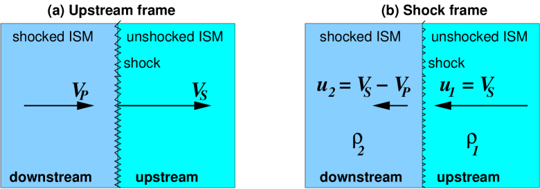
Figure 4: A shock moving with speed $V_{S}$ ahead of shocked gas moving at the pistion speed $V_{P}$ as seen (a) in the upstream frame, (b) in the shock frame.

In order to work out the energy gain per shock crossing, we can visualize magnetic irregularities tied to the plasma on either side of the shock as clouds of magnetized plasma of Fermi’s original theory (Fig. 5). Here, we assume that the shock is non-relativistic, such that we can make the approximation that the ultra-relativistic accelerated particles are isotropic in both upstream and downstream frames. By considering the rate at which cosmic rays cross the shock from downstream to upstream, and upstream to downstream, one finds $\langle\cos\theta_{1}\rangle\approx-2/3$ and $\langle\cos\theta_{2}^{\prime}\rangle\approx 2/3$, and Eq. 4 then gives

$${\langle\Delta E\rangle\over E}\simeq{4\over 3}\beta\simeq{4\over 3}{V_{P}\over c}\simeq{4\over 3}{(R-1)\over R}{V_{S}\over c}.$$ (13)

Note this is 1st order in $\beta=V_{P}/c$, and so the fractional energy change per collision can be much higher than in Fermi’s original theory. This is because of the converging flow – whichever side of the shock you are on, if you are moving with the plasma, the plasma on the other side of the shock is approaching you at speed $V_{p}$.

Figure 5: Interaction of cosmic ray of energy $E_{1}$ with a shock moving with speed $V_{s}$.

To obtain the energy spectrum we need to find the probability of a cosmic ray encountering the shock once, twice, three times, etc. If we look at the diffusion of a cosmic ray as seen in the rest frame of the shock (Fig. 6), there is clearly a net flow of the energetic particle population in the downstream direction.

Figure 6: Diffusion of cosmic rays from upstream to downstream seen in the shock frame.

The flux of cosmic rays lost downstream is

$$f_{{\rm loss}}=n_{\rm CR}V_{S}/R$$ (14)

since cosmic rays with number density $n_{\rm CR}$ at the shock are advected downstream with speed $u_{2}=V_{S}/R$ (from right to left in Fig. 6) and we have neglected relativistic transformations of the rates because $V_{S}\ll c$.

Upstream of the shock, cosmic rays travelling at speed $v$ at angle $\theta$ to the shock normal (as seen in the laboratory frame) approach the shock with speed $(V_{S}+v\cos\theta)$ as seen in the shock frame. Clearly, to cross the shock, $\cos\theta>-V_{S}/v$. Then, assuming cosmic rays upstream are isotropic, the flux of cosmic rays crossing from upstream to downstream is

$$f_{\rm cross} = n_{\rm CR}{1\over 4\pi}\int_{-V_{S}/v}^{1}(V_{S}+v\cos\theta)2\pi d(\cos\theta)\;\approx\;n_{\rm CR}v/4.$$ (15)

The probability of crossing the shock once and then escaping from the shock (being lost downstream) is the ratio of these two fluxes:

$${\rm Prob.(escape)}=f_{\rm loss}/f_{\rm cross}\approx 4V_{S}/Rv.$$ (16)

The probability of returning to the shock after crossing from upstream to downstream is

$${\rm Prob.(return)}=1-{\rm Prob.(escape)},$$ (17)

and so the probability of returning to the shock $m$ times and also of crossing the shock at least $m$ times is

$${\rm Prob.(cross}\geq m{\rm)}=[1-{\rm Prob.(escape)}]^{m}.$$ (18)

The energy after $m$ shock crossings is

$$E=E_{0}\left(1+{\Delta E\over E}\right)^{m}$$ (19)

where $E_{0}$ is the initial energy.

To derive the spectrum, we note that the integral energy spectrum (number of particles with energy greater than $E$) on acceleration must be

$$N(>E)\propto[1-{\rm Prob.(escape)}]^{m}$$ (20)

where

$$m={\ln(E/E_{0})\over\ln(1+\Delta E/E)}.$$ (21)

Hence,

$$\ln N(>E)=A+{\ln(E/E_{0})\over\ln(1+\Delta E/E)}\ln[1-{\rm Prob.(escape)}],$$ (22)

where $A$ is a constant, and so

$$\ln N(>E)=B-(\Gamma-1)\ln E$$ (23)

where $B$ is a constant and

$$\Gamma=\left(1-{\ln[1-{\rm Prob.(escape)}]\over\ln(1+\Delta E/E)}\right)\approx{R+2\over R-1}$$ (24)

where we have used $\ln(1+x)\approx x$ for $x\ll 1$.

Hence we arrive at the spectrum of cosmic rays on acceleration

$$N(>E)\propto E^{{-(\Gamma-1)}}\hskip 28.45274pt\rm(integral\;form)$$ (25)

$${dN\over dE}\propto E^{{-\Gamma}}\hskip 28.45274pt\rm(differential\;form).$$ (26)

For compression ratio $R=4$ (strong shock) we have the well-known $E^{-2}$ differential spectrum. The observed cosmic ray spectrum is steepened by energy-dependent escape of cosmic rays from the Galaxy.

2.3 Acceleration Rate

Here we again neglect effects of cosmic ray pressure and consider only a non-relativistic shock. The acceleration rate is defined by

$$r_{\rm acc}(E)\equiv{1\over E}\left.{dE\over dt}\right|_{\rm acc}={(\langle\Delta E\rangle/E)\over t_{\rm cycle}(E)}\approx{4\over 3}{(R-1)\over R}{V_{S}\over c\;t_{\rm cycle}(E)}$$ (27)

where $t_{\rm cycle}$ is the time for one complete cycle, i.e. from crossing the shock from upstream to downstream, diffusing back toward the shock and crossing from downstream to upstream, and finally returning to the shock.

The rate of loss of accelerated particles downstream is the probability of escape per shock crossing divided by the cycle time

$$r_{\rm esc}(E)={{\rm Prob.(escape)}\over t_{\rm cycle}}\approx{4\over R}{V_{S}\over c\;t_{\rm cycle}(E)}={3\over R-1}r_{\rm acc}(E)$$ (28)

We see immediately that the ratio of the escape rate to the acceleration rate depends on the compression ratio

$${r_{\rm esc}(E)\over r_{\rm acc}(E)}\approx{3\over R-1}=(\Gamma-1)$$ (29)

and for a strong shock ($R=4$) the two rates are equal, giving the well-known $E^{-2}$ power-law.

We shall discuss these processes in the shock frame (see Fig. 6) and consider first particles crossing the shock from upstream to downstream and diffusing back to the shock, i.e. we shall work out the average time spent downstream. Since we are considering non-relativistic shocks, the time scales are approximately the same whether measured in the upstream or downstream plasma frame, and so in this section we drop the use of subscripts indicating the frame of reference.

Diffusion takes place in the presence of advection at speed $u_{2}$ in the downstream direction. The diffusion coefficient will be a function of magnetic rigidity which, for ultra-relativistic particles considered in this paper, is approximately equal to $E/Ze$ where $Ze$ is the charge. However, here we are mainly concerned with singly charged particles and shall work in terms of $E$ rather than rigidity. The diffusion coefficient depends on the turbulence in the magnetic field. Often a power-law dependence $k(E)\propto E^{\delta}$ is assumed, where $\delta$ depends on the spectrum of turbulence. For a Kolmogorov spectrum $\delta=1/3$, and for a completely tangled magnetic field $\delta=1$ at least over some range of energies.

The typical distance a particle diffuses in time t is $\sqrt{k_{2}t}$ where $k_{2}$ is the diffusion coefficient in the downstream region. The distance advected in this time is simply $u_{2}t$. If $\sqrt{k_{2}t}\gg u_{2}t$ the particle has a very high probability of returning to the shock, and if $\sqrt{k_{2}t}\ll u_{2}t$ the particle has a very high probability of never returning to the shock (i.e. it has effectively escaped downstream). So, we set $\sqrt{k_{2}t}=u_{2}t$ to define a distance $k_{2}/u_{2}$ downstream of the shock which is effectively a boundary between the region closer to the shock where the particles will usually return to the shock and the region farther from the shock in which the particles will usually be advected downstream never to return. There are $n_{\rm CR}k_{2}/u_{2}$ particles per unit area of shock between the shock and this boundary. Dividing this by $f_{\rm cross}$ (Eq. 15) we obtain the average time spent downstream before returning to the shock

$$t_{2}(E)\approx{4\over c}{k_{2}(E)\over u_{2}}.$$ (30)

Consider next the other half of the cycle after the particle has crossed the shock from downstream to upstream until it returns to the shock. In this case we can define a boundary at a distance $k_{1}/u_{1}$ upstream of the shock such that nearly all particles upstream of this boundary have never encountered the shock, and nearly all the particles between this boundary and the shock have diffused there from the shock. Then dividing the number of particles per unit area of shock between the shock and this boundary, $n_{\rm CR}k_{1}/u_{1}$, by $f_{\rm cross}$ we obtain the average time spent upstream before returning to the shock

$$t_{1}(E)\approx{4\over c}{k_{1}(E)\over u_{1}},$$ (31)

and hence the cycle time

$$t_{\rm cycle}(E)\approx{4\over c}\left({k_{1}(E)\over u_{1}}+{k_{2}(E)\over u_{2}}\right).$$ (32)

The acceleration rate is then given by

$$r_{\rm acc}(E)\approx{(R-1)u_{1}\over 3R}\left({k_{1}(E)\over u_{1}}+{k_{2}(E)\over u_{2}}\right)^{-1}.$$ (33)

At this point, a comparison with stochastic acceleration is appropriate. Noting that the diffusion coefficient can be written

$$k={1\over 3}\lambda_{\rm coll}v={1\over 3}v^{2}/r_{\rm coll}$$ (34)

where $\lambda_{\rm coll}$ and $r_{\rm coll}$ are the effective collision mean free path and collision frequency, respectively, the acceleration rate can be written

$$r_{\rm acc}(E)\propto\left({u_{1}\over v}\right)^{2}r_{\rm coll}$$ (35)

which has the same functional form as for stochastic acceleration acceleration (Eq. 10) as pointed out by Jones (1994).

For either shock acceleration or stochastic acceleration to be able to accelerate cosmic rays to high energies the physical conditions must be suitable: Alfvén waves, magnetic irregularities or turbulence in the magnetic field must be present on length scales of the gyroradii of particles being accelerated and provide a sufficiently high scattering rate such that the required maximum energy can be achieved during the life-time of the accelerator, and the large-scale magnetic field must be able to confine the the highest energy particles within the accelerator. There are only a few places (solar flares) where the turbulence is likely to be strong enough for stochastic acceleration to work, and the spectrum will differ for different species. Generally, shock acceleration is favoured for the following reasons: (a) collisionless shocks exist everywhere, provide the necessary physical conditions, and are known to accelerate particles efficiently; (b) the energy associated with shocks can be large (a significant fraction of the energy released in a supernova explosion is carried by the supernova ejecta); (c) in the test particle case at least, the spectrum of accelerated particles is a power law which is the same for all species and depends only on the compression ratio (see Eq. 24).

2.4 Maximum Acceleration Rate

We next consider the diffusion for the cases of parallel, oblique, and perpendicular shocks, and estimate the maximum acceleration rate for these cases. The diffusion coefficients required, $k_{1}$ and $k_{2}$, are the coefficients for diffusion parallel to the shock normal. The diffusion coefficient along the magnetic field direction is some factor $\eta$ times the minimum diffusion coefficient, known as the Bohm diffusion coefficient,

$$k_{\parallel}=\eta{1\over 3}r_{g}c$$ (36)

where $r_{g}$ is the gyroradius, and $\eta>1$.

Parallel shocks are defined such that the shock normal is parallel to the magnetic field ($\vec{B}||\vec{u_{1}}$). In this case, making the approximation that $k_{1}=k_{2}=k_{\parallel}$ and $B_{1}=B_{2}$ one obtains

$$t_{\rm acc}^{\parallel}\approx{20\over 3}{\eta E\over eB_{1}u_{1}^{2}}.$$ (37)

For a shock speed of $u_{1}=0.1c$ and $\eta=10$ one obtains an acceleration rate (in SI units) of

$$\left.{dE\over dt}\right|_{\rm acc}\approx 1.5\times 10^{-4}ec^{2}B.$$ (38)

For the oblique case, the angle between the magnetic field direction and the shock normal is different in the upstream and downstream regions, and the direction of the plasma flow also changes at the shock. The diffusion coefficient in the direction at angle $\theta$ to the magnetic field direction is given by

$$k=k_{\parallel}\cos^{2}\theta+k_{\perp}\sin^{2}\theta$$ (39)

where $k_{\perp}$ is the diffusion coefficient perpendicular to the magnetic field. Jokipii (1987) shows that

$$k_{\perp}\approx{k_{\parallel}\over 1+\eta^{2}}$$ (40)

provided that $\eta$ is not too large ($\eta$ values up to $\sim$10), and that acceleration at perpendicular shocks can be much faster than for the parallel case. For a perpendicular shock ($\theta=90^{\circ}$), $k=k_{\perp}$ and $B_{2}\approx 4B_{1}$ and one obtains

$$t_{\rm acc}^{\perp}\approx{8\over 3}{E\over\eta eB_{1}u_{1}^{2}}.$$ (41)

For a shock speed of $u_{1}=0.1c$ and $\eta=10$ one obtains an acceleration rate (in SI units) of

$$\left.{dE\over dt}\right|_{\rm acc}\approx 0.04ec^{2}B.$$ (42)

Ellison, Baring and Jones (1995) have examined in detail the acceleration time and injection efficiency for oblique shocks. They point out that Eq. 33 is only valid when $k_{1}/u_{1}\geq r_{g}$ which requires that cosmic ray velocities, $v$, satisfy $\eta\leq v/u_{1}$. If this condition is not met, as would typically be the case for thermal particles if $\eta\gg 1$, then these particles would have a reduced probability of returning to the shock after crossing. As injection into the acceleration process is assumed to be from the thermal plasma, having particle speeds $v\sim u_{1}$, this will cause problems for the injection of cosmic rays in the case of highly oblique shocks. Thus, although having $\eta\gg 1$ can significantly reduce the acceleration time in oblique shocks, the injection efficiency would also be significantly reduced. Ellison, Baring and Jones (1995) find this to be a serious problem for $\theta>40^{\circ}$. One possible solution to this problem could be injection of a previously accelerated particle population, e.g. acceleration in a pulsar magnetosphere followed by injection into the supernova shock. Alternatively, injection from a supra-thermal tail of the thermal distribution could help, with the supra-thermal tail being due to heating by hard X-rays or gamma-rays from a nearby source.

Supernova shocks remain strong enough to continue accelerating cosmic rays for about 1000 years. The rate at which cosmic rays are accelerated is inversely proportional to the diffusion coefficient (faster diffusion means less time near the shock). For the maximum feasible acceleration rate, a typical interstellar magnetic field, and 1000 years for acceleration, energies of $10^{{14}}\times Z$ eV are in principle possible ($Z$ is atomic number) at parallel shocks, and $10^{{16}}\times Z$ eV at perpendicular shocks but in this case, as noted above, injection may be a problem.

2.5 Effect of Cosmic Ray Pressure

Inclusion of the effects of cosmic ray pressure on the shock profile, and consequently on the spectrum of accelerated particles, is a very difficult problem and we refer the reader to Jones & Ellison (1991) for a detailed discussion. The shock profile, instead of being a step-function becomes smoothed, and this affects the acceleration of low and high energy particles differently thereby affecting the cosmic ray spectrum. Generally, the results are sensitive to Mach number, fraction of energy flux of upstream plasma converted to accelerated particles, energy dependence of diffusion coefficient, etc. Calculated spectra may be $E^{-2}$, or flatter, or concave, depending on the input and the approximations made.

The original method of treating this non-linear effect is the two-fluid model (see e.g. the review by Drury 1983b), the two fluids being plasma with ratio of specific heats $\gamma$=5/3, and cosmic rays with $\gamma$=4/3. To solve the steady-state two-fluid equations it is necessary to make some approximations, usually that the cosmic rays interact with the gas only through their pressure, and that the cosmic ray pressure and energy flux are continuous across the shock. Furthermore an effective ratio of specific heats $\gamma_{\rm eff}$ and energy-independent diffusion was generally assumed. The solutions were often found to be unstable at high Mach numbers unless the spectrum was cut-off artificially, and the approximations used meant that there was, in effect, injection without conservation of particle number.

In time-dependent two-fluid model calculations (e.g. Falle & Giddings 1987, Bell 1987), $\gamma_{\rm eff}$ can be calculated self-consistently by weighting $\gamma$ by the pressures of the two fluids taking account of the spectrum of energetic particles, and energy-dependent diffusion can be included. Also, finite times for acceleration effectively eliminate the problem of injection without conservation of particle number. See Baring (1997) for a brief review and additional references, and Blandford and Eichler (1987), Berezhko (1999) and Berezhko and Völk (2000) for alternative approaches to this non-linear problem.

2.6 Relativistic Shocks

Shocks in jets of active galactic nuclei (AGN) and GRB are likely to be relativistic, i.e. $u_{1}>0.1c$, with shock Lorentz factors, $\Gamma\sim 10$ and $\Gamma\sim 300$, respectively. For relativistic plasma motion with bulk velocities comparable to those of the particles being accelerated, the particle distribution will not be isotropic, and the approximations used earlier are no longer valid. Instead, the typical escape probability and fractional energy gain per shock crossing are (very crudely) $\sim 0.5$ and $\sim 1$, respectively. Initial work on relativistic shock acceleration was done by Peacock (1981); see Kirk & Duffy (1999) for a topical review and additional references.

Figure 7: Momentum spectra obtained from Monte Carlo simulations with small angle scattering upstream for $\Gamma_{1}=10$ and $k\propto p$ ($\delta=1$). Spectra of particles which have escaped at times $t^{\prime}/t_{0}^{\rm sc}=10^{0},10^{1},\dots,10^{14}$ after injection are shown (solid histograms) together with the spectra of particles remaining in the acceleration zone (dotted histograms) at these times (adapted from Protheroe 2001).

The techniques used have been analytic (eigenfunction method) and Monte Carlo methods to solve the steady state equations for the particle spectral and angular distributions. The acceleration time depends strongly on $u_{1}$, $k_{\perp}/k_{\parallel}$, and $\theta$ and can be as low as $\sim(1$—10$)r_{g}/c$ (e.g. Bednarz & Ostrowski 1996, 1998, and Ostrowski 1998). Detailed studies have shown a trend in which shocks with larger $u_{1}$ generally have lower spectral indices (Kirk and Schneider 1987, Ellison and Jones 1990), and the spectral index can be very sensitive to the pitch angle particularly for mildly-relativistic shocks (see Baring 1997 for additional references). Nevertheless, for plane ultra-relativistic shocks, test-particle Monte Carlo simulations tend to give spectral indices close to $\Gamma=2.25$ (e.g. Bednarz & Ostrowski 1998, Gallant, Achterberg & Kirk 1999, Bednarz 2000, Kirk et al. 2000, Achterberg et al. 2001, Protheroe 2001, Meli and Quenby 2003a,2003b). These simulations assume strong turbulence downstream of the shock, but if this not present then the spectral index will be steeper (Ostrowski & Bednarz 2002).

Shock modification by the back-reaction of accelerated particles (Ellison & Double 2002) can cause the compression ratio to increase above the test particle value causing the spectrum of accelerated particles to differ from a simple power law with $\Gamma\approx 2.25$ for shock Lorentz factors less than 10.

A recent development has been to simulate separately the propagation upstream and downstream to work out the probability of returning to the shock at a particular angle to the shock normal for a given direction on crossing the shock (Protheroe 2001, Lemoine & Pelletier 2003), and use these distributions to simulate very efficiently relativistic shock acceleration over a large dynamic range in particle momentum. The time evolution of the momentum spectrum for injection at the shock, at time $t=0$, of highly relativistic mono-energetic particles which are isotropic in the upstream frame and have upstream-frame momentum $p_{0}$ as calculated by Protheroe (2001) is shown in Fig. 7. Here, as observed in the downstream frame these injected particles have a range of initial momenta distributed up to $\sim 2p_{0}^{\prime}$ where $p_{0}^{\prime}=\Gamma_{12}p_{0}$ ($\Gamma_{12}$ is the Lorentz factor for transforming between upstream and downstream frames). All distances are measured in units of the upstream scattering mean free path $\lambda^{\rm sc}_{0}$ and all times are measured in units of $t^{\rm sc}_{0}=\lambda^{\rm sc}_{0}/c$. The figure shows how the spectrum develops with time after injection, showing separately at each time indicated the spectrum of particles which have escaped, and (dotted curves) the spectrum of particles remaining within the acceleration zone (i.e. not having yet escaped downstream).

3 Interactions of High Energy Cosmic Rays

Interactions of cosmic rays with radiation are important both during acceleration when the resulting energy losses compete with energy gains by, for example, shock acceleration, and during propagation from the acceleration region to the observer. For UHE CR the most important processes are pion photoproduction and Bethe-Heitler pair production both on the CMBR, and synchrotron radiation. In the case of nuclei, photodisintegration on the CMBR is also important.

3.1 Nucleons

The mean interaction length, $x_{p\gamma}$, of a proton of energy $E$ is given by,

$${1\over x_{p\gamma}(E)}={1\over 8\beta E^{2}}\int_{\varepsilon_{\rm min}(E)}^{\infty}\frac{n(\varepsilon)}{\varepsilon^{2}}\int_{s_{\rm min}}^{s_{\rm max}(\varepsilon,E)}\sigma(s)(s-m_{p}^{2}c^{4})dsd\varepsilon,$$ (43)

where $n(\varepsilon)$ is the differential photon number density of photons of energy $\varepsilon$, and $\sigma(s)$ is the appropriate total cross section for the process in question for a centre of momentum (CM) frame energy squared, $s$, given by

$$s=m_{p}^{2}c^{4}+2\varepsilon E(1-\beta\cos\theta)$$ (44)

where $\theta$ is the angle between the directions of the proton and photon, and $\beta c$ is the proton’s velocity. For pion photoproduction $s_{\rm min}\approx 1.16$ GeV², and for Bethe-Heitler pair production the threshold is somewhat lower, $s_{\rm min}\approx 0.882$ GeV². For both processes, $s_{\rm max}\approx(m_{p}^{2}c^{4}+4\varepsilon E)$ which corresponds to a head-on collision of a proton of energy $E$ and a photon of energy $\varepsilon$.

The mean interaction lengths for both processes, $x_{p\gamma}(E)$, are obtained from Equation 43 for interactions in the CMBR and are plotted as dashed lines in Fig. 8(a). Dividing by the mean inelasticity of the collision, $\kappa(E)$, one obtains the energy-loss distances for the two processes (solid curves),

$${E\over dE/dx}={x_{p\gamma}(E)\over\kappa(E)}.$$ (45)

Figure 8: (a) Mean interaction length (dashed lines) and energy-loss distance (solid lines), $E/(dE/dx)$, for Bethe-Heitler pair production and pion photoproduction in the CMBR (lower and higher energy curves respectively). (From Protheroe and Johnson 1995). (b) Energy-loss distance of Fe-nuclei in the CMBR for pair-production (leftmost dashed line) and pion photoproduction (rightmost dashed line). Photodisintegration distances are given for loss of one nucleon (lower dotted curve), two nucleons (upper dotted line) as well as the total loss distance (thick curve) estimated by Stecker and Salamon (1999). The thin full curve shows an estimate over a larger range of energy (Protheroe, unpublished) of the total loss distance based on photodisintegration cross sections of Karakula and Tkaczyk (1993).

3.2 Nuclei

In the case of nuclei the situation is a little more complicated. The threshold condition for Bethe-Heitler pair production can be expressed as

$$\gamma>{m_{e}c^{2}\over\varepsilon}\left(1+{m_{e}\over Am_{p}}\right),$$ (46)

and the threshold condition for pion photoproduction can be expressed as

$$\gamma>{m_{\pi}c^{2}\over 2\varepsilon}\left({1+{m_{\pi}\over 2Am_{p}}}\right).$$ (47)

Since $\gamma=E/Am_{p}c^{2}$, where $A$ is the mass number, we will need to shift both energy-loss distance curves in Fig. 8(a) to higher energies by a factor of $A$. We shall also need to shift the curves up or down as discussed below.

For Bethe-Heitler pair production the energy lost by a nucleus in each collision near threshold is approximately $\Delta E\approx\gamma 2m_{e}c^{2}$. Hence the inelasticity is

$$\kappa\equiv{\Delta E\over E}\approx{2m_{e}\over Am_{p}},$$ (48)

and is a factor of $A$ lower than for protons. On the other hand, the cross section goes like $Z^{2}$, so the overall shift is down (to lower energy-loss distance) by $Z^{2}/A$. For example, for iron nuclei the energy loss distance for pair production is reduced by a factor $26^{2}/56\approx 12.1$.

For pion production the energy lost by a nucleus in each collision near threshold is approximately $\Delta E\approx\gamma m_{\pi}c^{2}$, and so, as for pair production, the inelasticity is factor $A$ lower than for protons. The cross section increases approximately as $A^{0.9}$ giving an overall increase in the energy loss distance for pion production of a factor $\sim A^{0.1}\approx 1.5$ for iron nuclei. The energy loss distances for pair production and pion photoproduction are shown for iron nuclei in Fig. 8(b)

Photodisintegration can be very important both during acceleration and propagation and has been considered in detail by Tkaczyk et al. (1975), Puget et al. (1976), Karakula and Tkaczyk (1993), Epele and Roulet (1998) and Stecker and Salamon (1999). The photodisintegration distance defined by $A/(dA/dx)$ taken from Stecker and Salamon (1999) is shown in Fig. 8(b) together with an estimate made over a larger range of energy by Protheroe (unpublished) of the total loss distance based on photodisintegration cross sections of Karakula and Tkaczyk (1993). Clearly, photodisintegration is the dominant loss process for iron nuclei.

4 Maximum Energies

Because of their much lower energy losses at a given energy, protons and nuclei can be accelerated to much higher energies than electrons for a given magnetic environment. For stochastic particle acceleration by electric fields induced by motion of magnetic fields $B$, the rate of energy gain by relativistic particles of charge $Ze$ can be written (in SI units) $dE/dt=\xi Zec^{2}B$ as in Eq. 1, where $\xi<1$ and depends on the acceleration mechanism; a value of $\xi=0.04$ might be achieved by first order Fermi acceleration at a perpendicular shock with shock speed $\sim 0.1c$.

The rate of energy loss by synchrotron radiation of a particle of mass $Am_{p}$, charge $Ze$, and energy $\gamma mc^{2}$ is

$$-\left.{dE\over dt}\right|_{\rm syn}={4\over 3}\sigma_{T}\left({Z^{2}m_{e}\over Am_{p}}\right)^{2}{B^{2}\over 2\mu_{0}}\gamma^{2}c.$$ (49)

Equating the rate of energy gain with the rate of energy loss by synchrotron radiation places one limit on the maximum energy achievable by electrons, protons and nuclei:

$$E_{e}^{\rm cut} = 6.0\times 10^{2}\xi^{1/2}\left({B\over{\rm 1\;T}}\right)^{-1/2}\hskip 14.22636pt{\rm GeV},$$ (50)

$$E_{p}^{\rm cut} = 2.0\times 10^{9}\xi^{1/2}\left({B\over{\rm 1\;T}}\right)^{-1/2}\hskip 14.22636pt{\rm GeV},$$ (51)

$$E_{Z,A}^{\rm cut} = 2.0\times 10^{9}\xi^{1/2}{A^{2}\over Z^{3/2}}\left({B\over{\rm 1\;T}}\right)^{-1/2}\,{\rm GeV}.$$ (52)

The cut-off energies of protons and iron nuclei allowed by synchrotron radiation losses are shown in Figs. 9(a) and 9(b) respectively, and are plotted against magnetic field for three values of $\xi$.

Figure 9: Maximum energy as a function of magnetic field of (a) protons and (b) iron nuclei for maximum possible acceleration rate $\xi=1$ (dashed), plausible acceleration at perpendicular shock $\xi=0.04$ (solid), and plausible acceleration at parallel shock $\xi=1.5\times 10^{-4}$ (dotted). Straight lines on the right give the limit from synchrotron loss, curved lines on the left give the limit from Bethe-Heitler pair production and pion photoproduction (protons) or photodisintegration (iron nuclei).

Equating the total energy loss rate for proton–photon interactions (i.e. the sum of pion production and Bethe-Heitler pair production) in Fig. 8(a) to the rate of energy gain by acceleration gives the maximum proton energy in the absence of other loss processes. This is shown in Fig. 9(a) for the three $\xi$ values. As can be seen, for a perpendicular shock it is possible in principle to accelerate protons to $\sim 10^{13}$ GeV in a $\sim 10^{-5}$ G field.

The effective loss distance given in Fig. 8(b) is used together with the acceleration rate for iron nuclei to obtain the maximum energy as a function of magnetic field. This is shown in Fig. 9(b). We see that for a perpendicular shock it is in principle possible to accelerate iron nuclei to $\sim 2\times 10^{14}$ GeV in a $\sim 3\times 10^{-5}$ G field. While this is higher than for protons, iron nuclei are likely to get photodisintegrated into nucleons of maximum energy $\sim 4\times 10^{12}$ GeV, and so there is not much to be gained unless the source is nearby.

Of course, potential acceleration sites need to have the appropriate combination of size (much larger than the gyroradius at the maximum energy), magnetic field, shock velocity (or other relevant velocity) and the time available for acceleration. These limits were obtained and discussed in some detail by Biermann and Strittmatter (1987). We emphasize that the cut-off energies estimated above apply to ideal conditions in which strong scattering occurs at all energies between injection and the cut-off energy; in reality, the $\xi$-values above are probably optimistic.

5 Spectral Shape near Maximum Energy

To determine the spectral shape near maximum energy we use the leaky-box acceleration model (Szabo and Protheroe 1994, Protheroe and Stanev 1998) which may be considered as follows. A particle of energy $E_{0}$ is injected into the leaky box. While inside the box, the particle’s energy changes at a rate $dE/dt=Er_{\rm acc}(E)$ and in any short time interval $\Delta t$ the particle has a probability of escaping from the box given by $\Delta tr_{\rm esc}(E)$. The energy spectrum of particles escaping from the box then approximates the spectrum of shock accelerated particles.

At time $t$ after injecting $N_{0}$ particles of momentum $E_{0}$ into the acceleration zone, the number of particles remaining in the acceleration zone, $N_{\rm rem}(t)$, is obtained by solving

$${dN_{\rm rem}\over dt}=-N_{\rm rem}(t)r_{\rm esc}[E(t)]$$

which has solution

$$N_{\rm rem}(t)=N_{0}\exp\left[-\int_{0}^{t}r_{\rm esc}[E(t)]dt\right]=N_{0}\exp\left[-\int_{E_{0}}^{E}r_{\rm esc}(E){dt\over dE}dE\right].$$

The spectrum of accelerated (escaping) particles is then

$${dN\over dE} = -{dN_{\rm rem}\over dt}{dt\over dE}={N_{\rm rem}[t(E)]r_{\rm esc}[E(t)]\over E\,r_{\rm acc}[E(t)]}$$

$${dN\over dE} = N_{0}{r_{\rm esc}(E)\over E\,r_{\rm acc}(E)}\exp\left[-\int_{E_{0}}^{E}{r_{\rm esc}(E)\over E\,r_{\rm acc}(E)}dE\right].$$ (53)

Let us consider first the case of no energy losses, interactions, or losses due to any other process. Assuming that the diffusion coefficients upstream and downstream have the same power-law dependence on energy, and using Eq. 29,

$$r_{\rm acc}=aE^{-\delta},\;\;\;r_{\rm esc}=(\Gamma-1)aE^{-\delta}.$$ (54)

Then the differential energy spectrum of particles which have escaped from the accelerator is given by

$$dN/dE = N_{0}(\Gamma-1)(E_{0})^{-1}(E/E_{0})^{-\Gamma},$$ (55)

for $(E>E_{0})$ where $\Gamma=(R+2)/(R-1)$ is the differential spectral index.

5.1 Cut-Off due to Finite Acceleration Volume, etc.

Even in the absence of energy losses, acceleration usually ceases at some energy due to the finite size of the acceleration volume (e.g. when the gyroradius becomes comparable to the characteristic size of the shock), or as a result of some other process. We approximate the effect of this by introducing a constant term to the expression for the escape rate:

$$r_{\rm esc}=(\Gamma-1)aE^{-\delta}+(\Gamma-1)aE_{\rm max}^{-\delta}.$$ (56)

where $E_{\rm max}$ is defined by the above equation and will be close to the energy at which the spectrum steepens due to the constant escape term. We shall refer to $E_{\rm max}$ as the “maximum energy” even though some particles will be accelerated to energies above this.

Following the same procedure as for the case of a purely power-law dependence of the escape rate, one obtains the differential energy spectrum of particles $(E>E_{0})$ escaping from the accelerator,

$${dN\over dE}\! = \!N_{0}(\Gamma-1)(E_{0})^{-1}(E/E_{0})^{-\Gamma}[1+({E/E_{\rm max}})^{\delta}]$$ (57)

$$\times\exp\left\{-{\Gamma-1\over\delta}\left[\left({E\over E_{\rm max}}\right)^{\delta}-\left({E_{0}\over E_{\rm max}}\right)^{\delta}\right]\right\}$$

for $\delta>0$ (Protheroe and Stanev 1998). We compare in Fig 10(a) the spectra for $\Gamma=2$ and $\delta$ ranging from $1/3$ to $1$, and note that the energy dependence of the diffusion coefficient has a profound influence on the shape of the cut-off. This smooth cut-off occurs over up to three decades in energy and its shape depends on the momentum dependence of the diffusion coefficients, and the intrinsic spectral index $\Gamma$ which depends on the compression ratio. Such a smooth cut-off has very recently been noted in test-particle Monte Carlo simulations of shock acceleration at shocks in a cylindrical jet geometry where there is sideways leakage out of the jet (Casse and Markowith, 2003).

Figure 10: (a) Differential energy spectrum for the case of a cut-off due to escape for $\Gamma=2$ and $\delta=1/3$ (solid curve), 2/3 (dotted curve) and 1 (dashed curve) – from Protheroe & Stanev (1998). (b) Differential energy spectrum for the case of a cut-off due to $E^{2}$ energy losses for $\Gamma=2$ and $\delta=1/3$ and $E_{\rm cut}/E_{\rm max}=10^{-5}$ (leftmost curve), $10^{-4}$, …, $10^{2}$ (rightmost curve).

5.2 Cut-Off due to Energy Losses

When continuous energy losses are included the spectrum is cut-off sharply at an energy at which the total rate of energy gain is zero. Depending on the spectral index, and momentum dependence of the diffusion coefficient, either a pile-up or a steepening in the spectrum occurs before the cut-off. To calculate the energy spectrum a term representing the energy-loss rate must be added to the acceleration rate,

$$r_{\rm acc}=aE^{-\delta}+\left.{dE\over dt}\right|_{\rm loss},$$ (58)

but since the physical size of the “box” increases with energy, synchrotron losses can cause a particle in the downstream region to effectively fall out of the box (Drury et al 1999). This process can be represented by an additional escape term in the escape rate. The acceleration zone extends distances $L_{1}(E)=k_{1}(E)/u_{1}$ and $L_{2}(E)=k_{2}(E)/u_{2}$ upstream and downstream of the shock. With the additional term in the rate of escape of particles due to energy loss,

$$r_{\rm esc} = (\Gamma-1)aE^{-\delta}+(\Gamma-1)aE_{\rm max}^{-\delta}+{1\over L_{1}(E)+L_{2}(E)}{dL_{2}\over dE}\left(-\left.\;{dE\over dt}\right|_{\rm loss}\right)$$ (59)

$$r_{\rm esc} = (\Gamma-1)a(E^{-\delta}+E_{\rm max}^{-\delta})+\delta{L_{2}\over L_{1}+L_{2}}r_{\rm loss}(E)$$ (60)

where $r_{\rm loss}(E)=-(dE/dt)_{\rm loss}/E$, and we adopt $L_{2}/(L_{1}+L_{2})=R/(1+R)$ following Drury et al. (1999).

For the case of synchrotron losses the result depends on the parameters $\delta$, $\Gamma$, $E_{0}$, $E_{\rm cut}$ and $E_{\rm max}$. As a result of the energy loss by particles near the cut-off energy, a pile-up in the spectrum may be produced just below $E_{\rm cut}$. The size of the pile-up will be determined by the relative importance of $r_{\rm acc}$ and $r_{\rm esc}$ at energies just below $E_{\rm cut}$. Numerical solution of Eq. 53 gives the results for $\Gamma=2$, $\delta=1/3$ and various $E_{\rm max}$ which are shown in Fig. 10(b).

One can use the Monte Carlo method to investigate the shape of the cut-off or pile-up which results when the nominal cut-off energy is determined by interactions rather than continuous energy losses. This technique was used by Protheroe and Stanev (1998) to investigate cut-offs in electron spectra due to inverse Compton scattering in the Klein-Nishina regime, and by Szabo and Protheroe(1994) to investigate cut-offs in the proton spectrum due to photoproduction in a radiation field. Results for $E_{\rm cut}=2\times 10^{12}$ GeV due to photoproduction on the CMBR are shown in Figure 11.

Figure 11: The spectrum of particles produced during acceleration (multiplied by $E^{2}$) per proton injected into the accelerator ($\Gamma=2$, $k\propto E$): protons (full curve), neutrons (dotted curve), charged pions (dashed curve) and neutral pions (chain curve). Results are shown for $E_{\rm cut}=2\times 10^{12}$ GeV due to photoproduction on the cosmic microwave background. (Adapted from figure 7 of Szabo and Protheroe 1994).

6 Cascading in Cosmic Radiation Fields

As well as particles being produced during the acceleration process as a result of interactions, during propagation to Earth cascading occurs and the accompanying fluxes of $\gamma$-rays and neutrinos must not exceed the observed flux or flux limits. By measuring the accompanying fluxes, we may well provide additional clues to the nature and origin of the highest energy cosmic rays (Waxman and Bahcall 1999, Mannheim et al. 2001). Hence it is important to calculate these fluxes resulting from cascading.

Figure 12: (a) The mean interaction length for pair production for $\gamma$-rays in: radio background calculated by Protheroe and Biermann 1996 (solid curves labelled R), radio background of Clark (1970) (dotted line); CMBR (2.7K), infrared and optical background (IR) (Malkan and Stecker 1998). The mean interaction length for double pair production (4e) in the CMBR (Protheroe and Johnson 1995) are also shown. (b) The mean interaction length (dashed line) and energy-loss distance (solid line), $E/(dE/dx)$, calculated by Protheroe and Johnson (1995) for electron-photon triplet pair production (TPP) and inverse-Compton scattering (IC) in the CMBR. The energy-loss distance for synchrotron radiation is also shown (dotted lines) for intergalactic magnetic fields of $10^{-9}$ (bottom), $10^{-10}$, $10^{-11}$, and $10^{-12}$ gauss (top).

There are several cascade processes which are important for UHE CR propagating over large distances through a radiation field: protons interact with photons resulting in pion production and pair production; electrons interact via inverse-Compton scattering and triplet pair production, and emit synchrotron radiation in the intergalactic magnetic field; $\gamma$-rays interact by photon-photon pair production. Energy losses due to cosmological redshifting of high energy particles and $\gamma$-rays can also be important, and the cosmological redshifting of the background radiation fields means that energy thresholds and interaction lengths for the above processes also change with epoch (see e.g. Protheroe et al. 1995).

The energy density of the extragalactic background radiation is dominated by the CMBR. Other components of the extragalactic background radiation are discussed in the review of Ressel and Turner (1990). The extragalactic radiation fields which are important for cascades initiated by UHE cosmic rays include the cosmic microwave background, the radio background and the infrared–optical background. The radio background was measured over thirty years ago (Bridle 1967, Clarke et al. 1970), but the fraction of this radio background which is truly extragalactic, and not contamination from our own Galaxy, is still debatable. Berezinsky (1969) was first to calculate the mean free path on the radio background. More recently Protheroe and Biermann (1996) have made a new calculation of the extragalactic radio background radiation down to kHz frequencies. The main contribution to the background is from normal galaxies and is uncertain due to uncertainties in their evolution. The mean free path of photons in this radiation field as well as in the microwave and infrared backgrounds is shown in Fig. 12(a).

Inverse Compton interactions of high energy electrons and triplet pair production can be modelled by the Monte Carlo technique (e.g. Protheroe 1986, Protheroe 1990, Protheroe et al. 1992, Mastichiadis et al. 1994), and the mean interaction lengths and energy-loss distances for these processes are given in Fig. 12(b). Synchrotron losses must also be included in calculations and the energy-loss distance has been added to Fig. 12(b) for various magnetic fields.

Where possible, to take account of the exact energy dependences of cross-sections, one can use the Monte Carlo method. However, direct application of Monte Carlo techniques to cascades dominated by the physical processes described above over cosmological distances takes excessive computing time. Another approach based on the matrix multiplication method has been described by Protheroe (1986) and developed in later papers (Protheroe and Stanev 1993, Protheroe and Johnson 1995). A Monte Carlo program is used to calculate the yields of secondary particles due to interactions with radiation, and spectra of produced pions are decayed to give yields of $\gamma$-rays, electrons and neutrinos. For the pion photoproduction interactions a new program called SOPHIA is available (Mücke et al. 1998).

7 Radio Galaxies and Active Galactic Nuclei

Rachen and Biermann (1993) have demonstrated that cosmic ray acceleration hotspots of giant radio lobes of Fanaroff-Riley Class II radio galaxies can fit the observed spectral shape and the normalization at 10 – 100 EeV to within a factor of less than 10. Protheroe and Johnson (1995) repeated Rachen and Biermann’s calculation to calculate the flux of diffuse neutrinos and $\gamma$-rays which would accompany the UHE cosmic rays as a result of pion photoproduction on the CMBR, and their calculated flux is shown in Fig. 13. The flux of extremely high energy neutrinos may give important clues to the origin of the UHE cosmic rays (for reviews of high energy neutrino astrophysics see Protheroe 1998 and Learned and Mannheim 2000). They may even be able to produce the observed UHE CR above the GZK threshold through interacting with cosmological neutrinos in our galactic halo as discussed in the next section on “Z-bursts”.

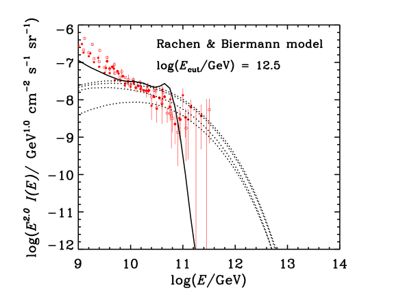
Figure 13: Cosmic ray proton intensity multiplied by $E^{2}$ in the model of Rachen and Biermann (1993) as calculated by Protheroe and Johnson (1995) for proton injection up to $3\times 10^{12}$ GeV (solid line). Also shown are intensities of neutrinos (dotted lines, $\nu_{\mu},\bar{\nu}_{\mu},\nu_{e},\bar{\nu}_{e}$ from top to bottom), and photons (long dashed lines). Data are from Gaisser and Stanev (1998).

AGN jets may also accelerate protons to ultra high energies and produce neutrino, gamma-ray and cosmic ray signals as a result of pion photoproduction interactions in the intense AGN radiation fields. There are different versions of these models in which the target photons are produced inside the blob, e.g. as synchrotron emission by a co-accelerated population of electrons (Mannheim 1993, 1995), or are external to the jet, e.g. from an accretion disk (Protheroe 1997). In addition, proton synchrotron blazar models in which the high energy part of the spectral energy distribution is mainly due to synchrotron radiation by protons have been proposed for some blazars (Mücke and Protheroe 2000, Mücke et al. 2001, Aharonian 2000). The relative contributions of various classes of AGN to the neutrino, gamma-ray and cosmic ray backgrounds are discussed by Mannheim et al. (2001).

Interestingly, Tinyakov & Tkachev (2001b, 2003) have claimed a correlation between the arrival directions of cosmic rays, having energies above 240 EeV from the Yakutsk array and above 480 EeV from the AGASA array, with the the directions of the 22 most powerful BL Lac objects with redshifts $z$$>$0.1. In this analysis, the energy cuts were those for which there was an indication of small-angle clustering from their previous analysis (Tinyakov & Tkachev 2001a). As pointed out by Evans, Ferrer & Sarkar (2003) the redshift cut implies that cosmic rays from these sources would be strongly affected by the GZK cut-off. Furthermore, cosmic rays propagating to Earth from large redshifts through the extragalactic magnetic field and CMBR may have difficulty in reaching us in a Hubble time as well as being severely affected by photoproduction interactions. Evans, Ferrer & Sarkar (2003) fail to find a statistically significant correlation between the cosmic ray arrival directions and the directions of BL Lac objects, and claim the correlation found by Tinyakov & Tkachev (2001b, 2003) to be spurious, and due to the cuts imposed on the data. We would add that there is no reason to limit searches to BL Lac objects as these objects are thought to be Fanaroff Riley Class I radio galaxies having jets closely aligned to our line of sight – unless the particles being searched for are neutral particles produced and relativistically beamed in the jets, there is no reason to favour BL Lac objects over the more numerous Fanaroff Riley Class I radio galaxies. The redshift cut ($z$$>$0.1) was used to ensure the BL Lac objects were powerful, but more powerful Fanaroff Riley Class I radio galaxies can appear less luminous than less powerful BL Lac objects, due to the absence of strong relativistic beaming of photons toward the observer. Excluding nearer BL Lac objects and Fanaroff Riley Class I radio galaxies seems to us to be illogical. Indeed, the sub-parsec scale jets of the nearby Fanaroff-Riley Class I radio galaxy M87, near the centre of the Virgo Cluster, may be a mis-aligned blazar of the BL Lac type, and may accelerate protons to ultra-high energies which could propagate to Earth if the magnetic field topology between our Galaxy and the Virgo Cluster were favourable (Protheroe, Donea and Reimer 2003).

Quasars are also an interesting possibility. Farrar and Biermann (1998) found a correlation between the arrival directions of the five highest energy cosmic rays having well measured arrival directions and radio-loud flat spectrum radio quasars with redshifts ranging from 0.3 to 2.2. The probability of obtaining the observed correlation by chance is estimated to be 0.5%. Although the statistical significance is not overwhelming, and indeed other researchers find no statistically significant evidence for such a correlation (Hoffman 1999, Sigl et al. 2001), if further evidence is provided for this correlation the consequences would be far reaching. The distances to these AGN are far in excess of the energy-loss distance for pion photoproduction by protons. Furthermore, given the existence of intergalactic magnetic fields, any charged particle would be significantly deflected and there should be no arrival direction correlation with objects at such distances. Hence, the particles responsible would need to be be stable, neutral, and have a very low cross section for interaction with radiation. Of currently known particles, only neutrinos fit this description, however supersymmetric particles are another possibility, as suggested by Farrar and Biermann (1998), although this possibility now appears to be ruled out (Gorbunov, Raffelt & Semikoz 2001).

7.1 Z-Bursts

The difficulty of having high energy neutrinos producing the highest energy cosmic rays directly is circumvented if the neutrinos interact well before reaching Earth and produce a particle or particles which will produce a normal looking air shower. As suggested by Weiler (1999), this may occur due to interactions with the 1.9 K cosmic background neutrinos (see also Gelmini and Kusenko 2000). The clustering of relic neutrinos in hot dark matter galactic halos would give an even denser nearby target for ultra high energy neutrinos as suggested by Fargion et al. (1999). The cross section is much larger for resonant $Z^{0}$ production which would occur for a UHE neutrino with energy $\sim m_{Z}^{2}/2m_{\nu}\sim 4\times 10^{21}/(m_{\nu}/$eV) eV. From the recent SNO results( Ahmad et al., 2002), the Super-Kamiokande atmospheric neutrino results (Toshito et al., 2001) and the tritium $\beta$ decay results (Bonn et al., 2001), Ahmad et al. (2002) concluded that the sum of mass eigenvalues of oscillating neutrinos was in the range 0.05–8.4 eV. Hence, the required UHE neutrino energy for resonant $Z^{0}$ production is very interestingly at or above the energies of UHE CR near the GZK cut-off. In this “Z-Burst” scenario, the $Z^{0}$ produced would have a comparable energy to the UHE neutrino, and decay into leptons and hadrons (including nucleons) which could be detected as UHE CR. In principle, there is also the possibility of the determination of absolute neutrino masses from Z-bursts if the galactic cosmic ray spectrum from normal acceleration were known (Päs and Weiler 2001, Fodor et al. 2002).

The main problem with the Z-Burst scenarios is that except for the case of unrealistic source models (production of UHE neutrinos with very few other UHE particles) or rather extreme over-densities (by $>$$10^{3}$) of relic neutrinos, the cascade gamma-ray flux would exceed the GeV gamma-ray intensity observed by EGRET (e.g. Kalashev et al. 2002). Also, extremely high fluxes of UHE neutrinos are required to explain the observed UHE CR spectrum. They are well in excess of those expected from AGN, and the possibility of explanation in terms of $X$ particle decay exclusively into neutrinos seems unsatisfactory (Berezinsky et al. 2002). Nevertheless, these fluxes are in principle detectable with existing neutrino detectors, and if they exist should certainly be detected with future large area cosmic ray detectors, such as the Pierre Auger Observatory, which are also sensitive to UHE neutrinos. If detected, the observed UHE neutrino flux, together with the observed UHE CR flux and anisotropy would place important constraints on the mass of the possible neutrino species forming the dark matter galactic halo, and its radial distribution (e.g. Singh and Ma 2003) as well as the source of the UHE neutrinos. Their detection would also require a re-evaluation of the our understanding of electromagnetic and hadronic cascading in the CMBR and other radiation fields.

8 Topological Defects

Topological defects (TD) such as monopoles, cosmic strings, monopoles connected by strings, etc., may be produced at the post-inflation stage of the early Universe. In the process of their evolution the constituent superheavy fields (particles) may be emitted through cusps of superconducting strings, during annihilation of monopole-antimonopole pairs, etc. These particles, collectively called X-particles, can be superheavy Higgs particles, gauge bosons and massive supersymmetric (SUSY) particles. These are generally very short-lived, and their decay followed by a hadronization cascade could produce an observable signal. Signals of TD origin would be affected by interactions/cascading during propagation over cosmological distances to Earth. Protheroe and Johnson (1996) pointed out the importance of including pair-synchrotron cascades in UHE CR propagation and, following their approach, Protheroe and Stanev (1996) showed that the $\gamma$-ray flux for many TD models of UHE CR exceeded that observed at 100 MeV energies for $B\geq 10^{-9}$ G.

There could be also superheavy quasi-stable particles with lifetimes larger (or much larger) than the age of the Universe. These particles could be produced by many mechanisms during the post-inflation epoch, and survive until the present epoch. One interesting process is the “gravitational production of super-heavy particles”, in which no interaction of X-particles is required. Also, string theories predict the existence of other super-heavy particles (“cryptons”) which are metastable and could in principle form part of the cold dark matter (CDM) (see, e.g., Kolb 1998, Ellis 2000). As with any other kind of CDM, super-heavy quasi-stable X-particles would cluster in galactic halos. The same clustering would also occur for some TD, such as monopolonium, monopole-antimonopole pairs connected by a string, and vortons. Cosmic ray signals from all these objects would reach us relatively attenuated. Perhaps the most promising WIMP CDM candidate is the lightest SUSY particle (LSP) with mass only 20–1000 GeV, and so would not produce UHE CR.

8.1 Fragmentation functions

TD such as cosmic strings, necklaces, etc., are extragalactic, and could produce an extragalactic signal through the decay of short-lived X-particles. TD which accumulate in galaxy halos (monopolonia, monopole-antimonopole-pairs and vortons) could produce a galactic signal through the annihilation/emission and decay of short lived X-particles which would in turn decay promptly into Standard Model (SM) states. Super-heavy quasi-stable particles ($\tau\gg t_{0}$) would decay similarly, and also be clustered as CDM in galactic halos.

The $X$ particle decay products annihilate and could give rise to a jet of hadrons, e.g.

$$X\to\left\{\begin{array}[]{c}W^{+}W^{-}\\ Z^{0}Z^{0}\\ \bar{q}q\\ e^{+}e^{-}\\ {\rm etc.}\end{array}\right\}\to\mbox{~{}2 jets}\to\left\{\begin{array}[]{l}\gamma{\rm-rays}\\ {\rm neutrinos}\\ \mbox{nucleons ($\sim 5\%$)}\\ {\rm electrons}\end{array}\right.$$

Energy spectra of the emerging particles, the “fragmentation functions”, were first calculated by Hill (1983). Each jet has energy $m_{X}c^{2}/2$, and so one defines a dimensionless energy for the cascade particles, $x=2E/m_{X}c^{2}$. The fragmentation function for “species a” is then defined as $dN_{a}/dx$. A very flat spectrum of particles results, and extends up to $\sim m_{X}c^{2}/2$. In the case of decay of CDM in galactic halos, the resulting UHE CR spectrum is proportional the fragmentation function for nucleons.

Figure 14: Fragmentation functions for hadronization of baryons normalized at $x=0.1$ to the recent QCD calculation of Sarkar and Toldra (2002) for $m_{X}=10^{12}$GeV (solid curve): Hill(1983) (dot-dashed curve); Berezinsky et al. (1997) MLLA approximation (short dashed curve); Monte Carlo results of Birkel and Sarkar (1998) for $m_{X}=10^{11}$GeV (solid histogram); Berezinsky and Kachelriess (2000) for $m_{X}=10^{12}$GeV SUSY-QCD (long dashed curve); Sarkar and Toldra (2002) for $m_{X}=10^{12}$GeV SUSY-QCD (dotted curve); Rubin (2000) $m_{X}=10^{12}$GeV QCD (dot-dot-dot-dashed curve).

Some recent calculations of the fragmentation functions used the Modified Leading Logarithm Approximation (MLLA) which is valid only for $x\ll 1$, and in more recent QCD calculations PYTHIA/JETSET (Singh and Ma 2003) or HERWIG Monte Carlo event generators were used. The fragmentation functions due to Hill (1983), and those of Berezinsky et al. (1997) based on the MLLA are compared in Fig. 14. Initially, the inclusion of the production of SUSY particles was done by putting 40% of the cascade energy above threshold for production of SUSY particles into LSP (Berezinsky and Kachelriess 1998), thereby steepening the fragmentation functions for normal particles at high energy. Birkel and Sarkar (1998) showed that even without inclusion of SUSY production there is a significant dependence on $m_{X}$, such that for high $m_{X}$ the fragmentation functions are steeper, as a direct consequence of the well-known Feynman scaling violation in QCD. Fragmentation functions calculated by Birkel and Sarkar (1998) using the HERWIG event generator have been added to Fig. 14, but this event generator is now known to overestimate production of nucleons by a factor $\sim$2–3,(Sarkar 2000, Rubin 2000). Recent calculations by Rubin (2000), Sarkar and Toldra (2002) and Berezinsky and Kachelriess (2000) (added to Fig. 14) have used improved treatments of SUSY particle production, and result in only $\sim 5$–12% of the cascade energy going into LSP. Very recently, Barbot & Drees (2003) have produced a complete set of fragmentation functions for any SUSY particle of the minimal supersymmetric extension of the standard model into protons, photons, electrons, neutrinos and the LSP.

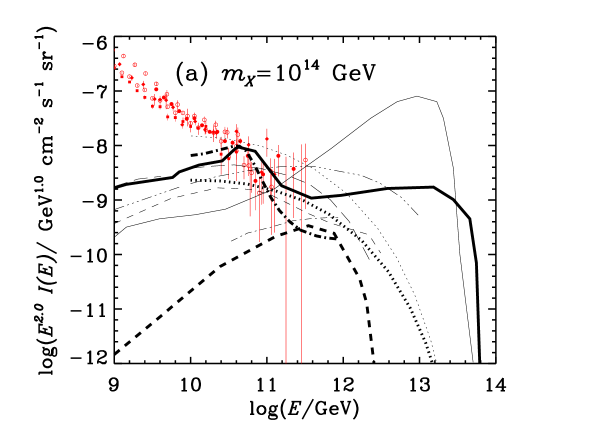
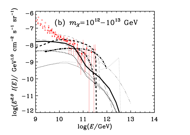
Figure 15: Predicted TD model spectra of protons (thick curves) and cascade photons (thin curves) compared with cosmic ray data from Gaisser and Stanev (1998). (a) $m_{X}=10^{14}$ GeV: Protheroe & Stanev (1996) (solid curves); Sigl et al. (1999) $X\to\nu\nu$ (short dashed curves); Blasi (1999) super-heavy relic halo population, SUSY-QCD and $\pi\mu e$ synchrotron (gamma rays only, long dashed curve), QCD and $\pi\mu e$ synchrotron (gamma rays only, dot-dot-dot-dashed curve); Berezinsky et al. (1998) super-heavy relic halo population, SUSY-QCD (dotted curves), necklaces SUSY-QCD (dot-dashed curves). (b) $m_{X}=10^{12}$–$10^{13}$ GeV: Sigl et al. (1999) $m_{X}=10^{13}$ GeV, $X\to q+q$ QCD (solid curves), $m_{X}=10^{13}$ GeV, $X\to q+l$ QCD (dotted curves); Blasi (1999) $m_{X}=10^{13}$ GeV super-heavy relic halo population, SUSY-QCD and $\pi\mu e$ synchrotron (gamma rays only, long dashed curve), QCD and $\pi\mu e$ synchrotron (gamma rays only, dot-dot-dot-dashed curve); Sarkar and Toldra (2002) super-heavy relic halo population QCD best fit $m_{X}=10^{12}$ GeV (protons only, leftmost dot-dashed curve) and SUSY-QCD best fit $m_{X}=5\times 10^{12}$ GeV (rightmost dot-dashed curve).

8.2 Viability of Dark Matter Origin of UHECR

Predictions for some TD and massive relic particles are show in Fig. 15. If CDM consists of particles associated with TD distributed uniformly throughout the Universe, then UHE CR are subject to the GZK cut-off. In this case $\gamma$-ray signals result from a pair-synchrotron cascade in background radiation and extragalactic magnetic fields. The magnetic fields used in some cascade calculations may have been unrealistically low, and it does appear difficult to explain the super-GZK events with such TD models without the flux of cascade gamma-rays exceeding the observed 100 MeV gamma-ray background.

Most of the matter in the Universe is CDM, and if it consists of massive relic particles they should cluster in galaxy halos. In this case, decay of massive relic particles would produce UHECR signals weakly anisotropic toward the GC, and the UHE CR spectrum would not have a GZK cut-off. Of the “top down” scenarios, these models currently seem to us to be the most viable. See Sarkar and Toldra (2002) for recent work on decay of superheavy dark matter particles.

9 Propagation through Magnetic Fields

Cosmic rays reach us after travelling through the magnetic fields which pervade space. Details of the strength and structure of such fields are unknown but broad generalizations are possible within certain volumes of the Universe.

Our galaxy is of spiral structure and the galactic magnetic field has a regular component with a characteristic strength of the order of microgauss and which seems to be associated with the spiral arms. Additionally, there is a turbulent, random, component which is at least as strong as the regular component. This component is even less well known since measurements of Faraday rotation or other techniques tend to average out when the line of sight transits a number of turbulence cells. The spectrum of turbulence scales is often assumed to be of a Kolmogorov kind which has the important property of being dominated by the largest scale sizes. Within our Galaxy, the largest internal structures tend to be of 100 pc scales (e.g. supernova remnants). With a field strength of a few microgauss, this means that significant scattering of cosmic rays will occur at least to a few times $10^{17}$eV since a proton with this energy has a gyroradius of 100 pc in a 1 $\mu$G field. Hence, the largest scale lengths in the turbulence of the Galactic magnetic field tend to dominate the propagation of the (more energetic) UHE CR in the Galaxy.

The particles follow paths rather like random walks up to the scale size of the turbulence. A first approximation to galactic propagation is then diffusion. Honda (1987) has given an excellent discussion of extensions to make the simple picture more realistic. That work, and similar propagation modelling by Clay (2000), gives us some understanding of resulting measurable properties of the cosmic ray beam. Since the propagation is diffusive, the time for a particle to leave the galaxy is greater than the simple direct transit time. This containment time increase results in an increase in flux over that which would have been observed had there only been straight line propagation from galactic sources. Containment time calculations thus allow us to crudely determine a ’source spectrum’. In one recent analysis (Clay 2000), the source spectrum shows no knee and, possibly, no ankle. It may be that both those features (and certainly the knee) are consistent with purely propagation effects. The resulting source spectrum is a power law with an index of 2. There is a problem with such an explanation for the ankle since particles above that energy travel in rather straight lines and a ’Milky Way’ perhaps ought to be visible in the anisotropy data. However, data at these energies are somewhat sparse and, of course, the AGASA/SUGAR source (Hayashida et al. 1999, Bellido et al. 2001) could be just such an effect.

Figure 16: Angular distribution of the arrival angle at Earth for mono-energetic injection of protons of energy $E=10^{21.5}$ eV, and for various source distances as indicated (from Stanev et al. 2000).

In considering the propagation from extragalactic sources, there are two environments to consider. They are the intra-cluster magnetic fields of both the source galaxy and our own galaxy, and the inter-cluster field. Clarke et al. (2001) have shown that, remarkably, a characteristic intra-cluster magnetic field strength in a rich galactic cluster fills the cluster and has microgauss strengths – maybe $5\mu$G in the inner 500 kpc. If we make a first approximation to a diffusion coefficient to be a factor $\eta\!>\!1$ times the minimum (Bohm) diffusion coefficient, i.e. $\eta r_{g}c/3$, we can assume diffusive propagation and derive an estimate of the time to reach a given root-mean-square displacement. If we consider a $10^{19}$eV particle in the $5\mu$G field, we find a required time of $10^{8}/\eta$ yr just to leave the source cluster through 500 kpc. The GZK effect is clearly relevant here. If the source is in the Virgo Cluster of galaxies, a cosmic ray must then travel through intercluster space and then reach us though our own cluster field. It may be that the intercluster field is also at significant levels. In this case, we are looking at tens of megaparsec from the nearest likely AGN source with a transit time, being dependent on the square of the distance, and becoming greater than the age of the Universe. This is clearly an issue which pushes us to a careful consideration of very local sources.

This argument is rather crude. Sigl (2000) has modelled time delays for particles travelling 10 Mpc in a turbulent $0.3\mu$G field. Even for that modest field strength, transit times of $10^{8}$ yr apply at 10–100 EeV. Apart from any concern about particles reaching us within the age of the Universe, our comments on diffusion times emphasize that it may not make sense to correlate cosmic ray observations with sources beyond 10 Mpc unless one can be sure that those sources have a lifetime for emission substantially greater than $10^{8}$yr. Monte Carlo calculations have been made by Stanev et al. (2000) for propagation through an irregular magnetic field having a Kolmogorov spectrum of turbulence with minimum wavenumber 1 Mpc^-1 and energy density equal to that of a much smaller 1 nG intergalactic field. Propagation from sources at several distances take account of diffusion in this turbulent field as well as interactions with the CMBR using the SOPHIA event generator (Mücke et al. 2000) and redshifting, and give the distributions in energy, time delay relative to straight-line propagation, and angular distribution about source direction. Fig. 16 shows the angular distribution of protons with initial energies 300 EeV arriving from sources at distances 2 Mpc, 8 Mpc, …512 Mpc away.

The situation is quite different if the intergalactic magnetic field structure is based on the observation of microgauss fields in clusters of galaxies (Kronberg 1994), and of clusters occurring in networks of “walls” separated by “voids”. Using a wall/void model similar to that of Medina Tanco (1998), Protheroe et al. (2003) discuss propagation from M87 (located close to the centre of the Virgo Cluster) assuming that it and our galaxy are embedded in the same wall (thickness 2.5 Mpc) which has a regular magnetic field of $10^{-7}$ G in the plane of the wall and $10^{-10}$ G in the surrounding void, and an irregular component with 30% of the energy density of the regular component and having a Kolmogorov spectrum of turbulence. Modelling M87 as a mis-aligned BL Lac object, they found the UHECR output from M87 to be at a level such that if UHECRs travelled in straight lines they would give an average intensity at Earth a factor $\sim$20 below that observed. However, observed fluxes will be very different for propagation in a more realistic magnetic field structure such as that described above. Propagation results for the wall/void model are shown for two initial energies $10^{19}$ eV and $10^{20}$ eV in Fig. 17. Note that Fig. 17 does not give the anisotropy that would be observed at the Earth due to cosmic rays from M87, but rather the enhancement factor (relative to straight line propagation) of the cosmic ray flux from M87 at positions on a sphere of radius 16 Mpc centred on M87. Enhancement factors $\sim$$10^{3}$ exist if the Earth is within $\sim$$1.5$ Mpc of a field line originating at M87. If this (rather special) condition were met M87 could easily explain the observed UHECR. Because of its very high black hole mass M87 was probably much more active at earlier times than at present (many objects exhibit a high state for $\sim$5% of the time) which makes M87 a more attractive candidate source of the UHECR.

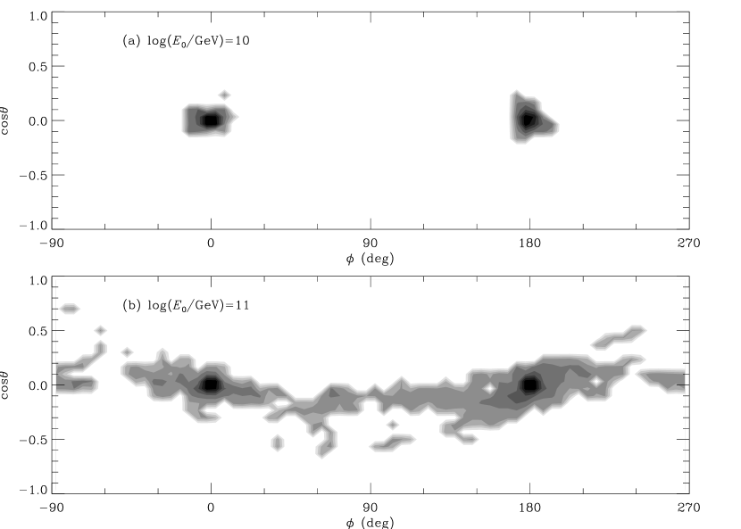
Figure 17: Enhancement factor relative to rectilinear propagation as a function position $(\cos\theta,\phi)$ a sphere of radius $\sim 16$ Mpc centred on the origin for protons of initial energy (a) $E_{0}=10^{19}$ eV and (b) $E_{0}=10^{20}$ eV injected isotropically at the origin in the wall/void model of the IGMF discussed in the text. Positions $(0,0^{\circ})$ and $(0,180^{\circ})$ are on the field line threading M87 (from Protheroe et al. 2003).

10 Conclusions

Cosmic ray astrophysics at the highest energies is entering a new era with major new facilities being proposed and developed. The tiny flux of particles in this range of energies challenges our understanding of the astrophysics which we apply to many other studies. We are led to examine processes in extreme regions such as the various components of AGN, to ask how particle acceleration may take place there, and to ask for detailed information on photon and magnetic fields throughout our local universe. This challenging work now truly complements studies throughout photon astrophysics.

References

Abu-Zayyad, T. et al. 2001, ApJ, 557, 686

Abu-Zayyad, T. et al. 2003, Submitted to Astropart. Phys., astro-ph/0208301

Achterberg, A., Gallant, Y.A., Kirk, J.G., Guthmann, A.W. 2001, MNRAS, 328, 393

Aharonian, F.A., Bhattacharjee P., & Schramm D.N. 1992, Phys. Rev. D, 46, 4188

Aharonian, F. 2000, New Astron., 5, 377

Ahmad, Q.R., et al., 2002, Phys. Rev. Lett., 89, 011301; Phys. Rev. Lett., 89, 011302

Anchordoqui, L.A., Dova, M.T., Epele, L.N., & Swain, J.D. 1998, Phys. Rev. D, 57, 7103

Auger Collaboration Contribution 2001, in Proceedings of XXVII Cosmic Ray Conference, Hamburg, Edited by M. Simon et al., Copernicus Gesellschaft 2001, Vol. 2, pp 699-787

Axford, W.I., Lear, E., & Skadron, G. 1977, in Proc. 15th Int. Cosmic Ray Conf., Plovdiv vol. 11, p 132

Barbot, C.& Drees, M., 2003, Astropart. Phys., 20, 5

Baltrusaitis, R.M. et al. 1985, Nucl. Instr. Meth., A240, 410

Baring, M.G. 1997, in Proc. of XXXIInd Rencontres de Moriond, “Very High Energy Phenomena in the Universe”, eds. Giraud-Heraud, Y. & Tran Thanh Van, J., (Editions Frontieres, Paris, 1997), p. 97

Bednarek, W., & Protheroe, R.J., 2002, Astropart. Phys., 16, 397

Bednarz, J., & Ostrowski, M. 1996, MNRAS, 283, 447

Bednarz, J., & Ostrowski, M. 1998, Phys. Rev. Lett., 80, 3911

Bednarz, J. 2000, MNRAS, 315, 37

Bell, A.R. 1978, MNRAS, 182, 443

Bell, A. R., & Lucek, S. G. 1996, MNRAS, 283, 1083

Bellido, J.A., Clay, R.W., Dawson, B.R., & Johnston-Hollitt, M. 2001, Astropart. Phys., 15, 167

Berezhko, E.G., & Krymski, G.F. 1988, Usp. Fiz. Nauk, 154, 49

Berezhko, E. G. 1994, Astron. Lett., 20, 75

Berezhko, E.G. 2001, Space Sci. Rev., 99, 295

Berezhko, E.G. & Völk, H.J. 2000, A&A, 357, 283

Berezinsky, V.S. 1970, Sov. J. Nucl. Phys., 11, 222

Berezinsky, V., Blasi, P., & Vilenkin, A. 1998, Phys. Rev. D, 58, 103515

Berezinsky, V., Kachelriess, M., & Vilenkin A. 1997, Phys. Rev. Lett., 79, 4302

Berezinsky, V., & Kachelriess, M. 1998, Phys. Lett. B, 434, 61

Berezinsky, V., & Kachelriess, M. 2001, Phys. Rev. D, 63, 034007

Berezinsky, V., Kachelreiss, M., & Ostapchenko, S. 2002, Phys. Rev. Lett., 89 171802

Bhattacharjee, P. & Sigl, G. 2000, Phys. Rep., 327, 109

Birkel, M., & Sarkar, S. 1998, Astropart. Phys., 9, 297

Blandford, R.D., & Ostriker, J.P. 1978, ApJ, 221, L29

Blandford, R, & Eichler, D. 1987, Phys. Rep., 154, 1

Blasi, P. 1999, Phys. Rev. D, 60, 123514

Blasi, P., Epstein, R. I., & Olinto, A. V., 2000, ApJ, 533, L123

Biermann, P.L., & Strittmatter, P.A. 1987, ApJ., 322, 643

Bird, D.J. et al. 1995, ApJ., 441, 144

Bonn, J. et al. 2001, Nucl. Phys. B Proc. Suppl., 91, 273

Bridle, A.H. 1967, MNRAS, 136, 14

Casse, F., & Markowith, A. 2003, A&A, 404, 405

Clarke, T.A., Brown, L.W. & Alexander, J.K. 1970, Nature, 228, 847

Clarke, T.E., Kronberg, P.P., & Bohringer, H. 2001, ApJ, 547, L111

Clay, R.W., McDonough, M.-A., & Smith, A.G.K. 1998, Pub. Astron. Soc. Aust., 15, 208

Clay, R.W. 2000, Pub. Astron. Soc. Aust., 17, 212

Clay, R.W. 2002, Pub. Astron. Soc. Aust., 19, 228

de Gouveia Dal Pino, E. M., & Lazarian, A. 2001, ApJ, 560, 358

Dermer, C.D. 2002, ApJ, 574, 65

Drury, L.O’C. 1983a, Space Sci. Rev., 36, 57

Drury, L.O’C. 1983b, Rep. Prog. Phys., 46, 973

Drury, L.O’C., Duffy, P., Eichler, D., & Mastichiadis, A. 1999, A&A, 347, 370

Elbert, J.W., & Sommers, P. 1995, ApJ, 441, 151

Ellis J. 2000, in Proc. of the 26th Int. Cosmic Ray Conf., AIP Conf. Proc. 516, Eds. B.L. Dingus et al. (American Inst. Physics), p 21

Ellison, D.C, & Eichler, D. 1984, ApJ, 286, 691

Ellison, D.C, Jones, F.C., & Reynolds, S.P. 1990, ApJ, 360, 702

Ellison, D.C., Baring, M.G., & Jones, F.C. 1995, ApJ, 453, 873

Ellison, D.C., & Double, G.P. 2002, APh, 18, 213

Epele, L.N., & Roulet, E. 1998, J. High Energy Phys., 9810, 9

Evans, N.W., Ferrer, F., & Sarkar, S., 2003, Phys. Rev., D67, 103005

Falcke, H., & Gorham, P. 2003, Astropart. Phys., 19, 477

Fargion, D., Mele, B., & Salis, A. 1999, ApJ, 517, 725

Farrar, G.R., & Biermann P.L. 1998, Phys. Rev. Lett., 81, 3579; erratum 1999, Phys. Rev. Lett., 83, 2478; Phys. Rev. Lett., 83, 1999, 2472 (response to Hoffman 1999)

Fodor, Z., Katz, S.D., & Ringwald, A. 2002, JHEP, 0206 046

Gaisser, T.K. 1990, “Cosmic Rays and Particle Physics”, (Cambridge University Press, Cambridge, 1990).

Gaisser T.K., & Stanev T. 1998, Europhys. J., 3, 1

Galama, T.J., et al. 1998, Nature, 395, 670

Gallant, Y. A., Achterberg, A., & Kirk, J. 1999, A&AS, 138, 549

Gelmini, G., & Kusenko, A. 2000, PRL, 84 1378

Gold, T., 1975 Phil. Trans. Roy. Soc., Series A, 277, 453

Gorbunov, D.S., Raffelt, G.G., & Semikoz, D.V., 2001, Phys. Rev., D64, 096005

Greisen, K. 1966, Phys. Rev. Lett., 16, 748

Halzen F., Vazquez R.A., Stanev T., & Vankov H.P. 1995, Astropart. Phys., 3, 151

Haswell, C.A., Tajima, T., & Sakai, J.-L. 1992, ApJ, 401, 495

Hayashida, N. et al. 1999, Astropart. Phys., 10, 303

Hill, C.T. 1983, Nucl. Phys. B, 224, 469

Hillas, A.M. 1984, Ann. Rev. Astron. Astrophys., 22, 425

Hoffman, C.M. 1999, Phys. Rev. Lett., 83, 2471

Honda, M. 1987, ApJ., 319, 836

Jokipii, J.R., & Morfill G.E. 1985, ApJ, 290, L1

Jokipii, J.R. 1987, ApJ, 313, 842

Jones, F.C., & Ellison, D.C. 1991, Space Sci. Rev., 58, 259

Jones, F.C. 1994, ApJS, 90, 561

Karakula, S., & Tkaczyk, W. 1993, Astropart. Phys., 1, 229

Kawabata, K.S. et al. 2003, astro-ph/0306155

Kirk, J.G., & Schneider, P. 1987, ApJ, 315, 425

Kirk, J.G., & Duffy, P. 1999, JPhG, 25, 163

Kirk, J.G., Guthmann, A.W., Gallant, Y.A., & Achterberg, A. 2000, ApJ, 542, 235

Kolb, E.W. 1998, in Proceedings of the NATO Advanced Study Institute on Techniques and Concepts of High-Energy Physics (10th: 1998: St. Croix, V.I.) Ed. T. Ferbel.

Kronberg, P.P. 1994, Rep. Prog. Phys.  57, 325

Krymsky, G.F. 1977, Dokl. Akad. Nauk. SSSR, 243, 1306

Learned, J., & Mannheim, K. 2000, Ann. Rev. Nucl. Part. Sci., 50, 679

Lemoine, M., & Pelletier, G. 2003, ApJ, 589, 73

Linsley, J. 1975, Phys. Rev. Lett., 34, 1530

Malkan M.A., & Stecker F.W, 1998, ApJ 496, 13

Mannheim K. 1993, A&A, 269, 67

Mannheim K. 1995, Astropart. Phys., 3, 295

Mannheim, K., Protheroe, R.J., & Rachen, J.P. 2001, Phys. Rev. D, 63, id. 023003

Mastichiadis, A., Protheroe, R.J. & Szabo, A.P. 1994, MNRAS, 266, 910

Medina Tanco, G.A. 1998, ApJ, 505, L79

Meli, A., & Quenby, J., 2003, Astropart. Phys., 19, 637

Meli, A., & Quenby, J., 2003, Astropart. Phys., 19, 649

Mücke, A., Engel, R., Rachen, J.P., Protheroe, R.J., & Stanev, T., 2000, Comp. Phys. Com., 124, 290

Mücke, A. & Protheroe, R.J. 2001, Astropart. Phys., 15, 121 Mücke, A., Protheroe, R.J., Engel, R., Rachen, J.P., & Stanev, T. 2003, Astropart. Phys., 18, 593

Müller, D., Swordy, S.P., Meyer, P., L’Heureux, J., & Grunsfeld, J.M., 1991, ApJ, 374, 356

Nagano, M., & Watson, A.A. 2000, Rev. Mod. Phys., 72, 3, 689

Norman, C.A., Melrose, D.B., & Achterberg, A. 1995, ApJ, 454, 60

Ostrowski, M. 1999, in Proc. Vulcano Workshop 1998: Frontier Objects in Astrophysics and Particle Physics, 1998 in Vulcano. Edited by F. Giovannelli & G. Mannocchi. Ital. Phys. Soc. Conf. Proc., Vol. 65. (Bologna, Italy: Italian Physical Society, 1999), p. 313

Ostrowski, M., & Bednarz, J. 2002, A&A, 394, 1141

Päs, H., & Weiler, T.J. 2001, Phys. Rev. D, 63, id. 113015

Peacock, J.A. 1981, MNRAS, 196, 135

Protheroe, R.J. 1986, MNRAS, 221, 769

Protheroe, R.J. 1990, MNRAS, 246, 628

Protheroe, R.J., Mastichiadis A. & Dermer C.D. 1992, Astropart. Phys., 1, 113

Protheroe, R.J., & Stanev, T.S. 1993, MNRAS, 264, 191

Protheroe, R.J., & Johnson, P.A. 1995, Astropart. Phys., 4, 253; erratum 1996,Astropart. Phys., 5, 215

Protheroe, R.J., Stanev, T., & Berezinsky, V.S. 1995, Phys. Rev. D, 51, 4134

Protheroe R.J., & Johnson P. 1996, Astropart. Phys., 4, 253

Protheroe, R.J., & Biermann, P.L. 1996, Astropart. Phys., 6, 45

Protheroe R.J., & Stanev T. 1996, Phys. Rev. Lett., 77, 3708; erratum 1997, Phys. Rev. Lett., 78, 2420

Protheroe R.J., 1997, in “Accretion Phenomena and Related Outflows”, IAU Colloquium 163, ed. D.T. Wickramasinghe, G.V. Bicknell, & L. Ferrario 1997, ASP Conf. Ser., Vol. 121, p. 585

Protheroe, R.J. 1998, in 18th Int. Conf. on Neutrino Physics and Astrophysics (Neutrino 98), Takayama, Nucl. Phys. B Proc. Suppl., 77, 465

Protheroe, R.J., & Stanev, T. 1999, Astropart. Phys., 10, 185

Protheroe, R.J., in “Topics in cosmic-ray astrophysics” ed. M.A. DuVernois, Nova Science Publishing: New York, 2000, pp 258–298

Protheroe, R.J. 2001, in Proceedings of XXVII Cosmic Ray Conference, Hamburg, Edited by M. Simon et al., Copernicus Gesellschaft 2001, Vol. 6, p. 2006, and ibid, Vol. 6, p. 2014

Protheroe, R.J., Donea, A.-C., & Reimer, A. 2003, Astropart. Physics, 19, 559

Puget, J.L., Stecker, F.W., & Bredekamp, J.H. 1976, ApJ, 205, 638

Rachen, J.P., & Biermann, P.L., 1993, A&A, 272, 161

Ressell, M.T., & Turner, M.S. 1990, Comm. Astrophys., 14, 323

Rubin, N. 1999, M. Phil. Thesis, University of Cambridge

Sarkar, S. 2000, in COSMO-99, in Third Intern. Workshop on Particle Physics and the Early Universe, p. 77, hep-ph/0005256

Sarkar, S., & Toldra, R. 2002, Nucl. Phys. B, 621, 495

Sigl G. et al. 1997, Phys. Lett. B, 392, 129

Sigl, G., Lee, S., Bhattacharjee, P., & Yoshida, S. 1999, Phys. Rev. D, 59, id. 043504

Sigl, G. 2000, Lect. Notes Phys., 556, 259

Sigl, G., Torres, D.F., Anchordoqui, L.A., & Romero, G.E 2001, Phys. Rev.  D, 63, id. 081302

Singh, S., & Ma, C-P. 2003, Phys. Rev., D 67, 023506

Smith, A.G.K., & Clay, R.W. 1997, Aust. J. Phys., 50, 827

Sorrell, W.H. 1987, ApJ., 323, 647

Stanev, T., Biermann, P.L., Lloyd-Evans, J., Rachen, J.P., & Watson, A.A. 1995, Phys. Rev. Lett., 75, 3056

Stanev, T., Engel, R., Mücke, A., Protheroe, R.J., & Rachen, J.P. 2000, Phys. Rev. D, 62, 093005

Stecker, F.W., & Salamon, M. 1999, ApJ, 512, 521

Szabo, A.P., & Protheroe, R.J. 1994, Astropart. Phys., 2, 375

Takeda, M. et al. 2003, Astropart. Phys., 19, 447

Tinyakov, P.G., & Tkachev, I.I., 2001a, JETP Lett., 74, 1

Tinyakov, P.G., & Tkachev, I.I., 2001b, JETP Lett., 74, 445

Tinyakov, P.G., & Tkachev, I.I., 2003, astro-ph/0301336

Tkaczyk, W., Wdowczyk, J., & Wolfendale, A.W. 1975, J. Phys. A, 8, 1518

Toshito, T. et al. 2001, hep-ex/0105023

Totani, T. 1999, Astropart. Phys., 11, 451

Vietri, M. 1995, ApJ, 453, 883

Waxman, E., & Bahcall, J. 1999, Phys. Rev. D, 59, id. 023002

Weiler, T. 1999, Astropart. Phys., 11 303

Zatsepin, G.T., & Kuzmin, V.A. 1966, Sov. Phys. JETP Lett., 4, 78