Modification of Projected Velocity Power Spectra by Density Inhomogeneities in Compressible Supersonic Turbulence

Abstract

The scaling of velocity fluctuation $\delta v$ as a function of spatial scale $\ell$ in molecular clouds can be measured from size-linewidth relations, principal component analysis, or line centroid variation. Differing values of the power law index of the scaling relation $\langle\delta v^{2}\rangle^{1/2}\propto\ell^{\gamma_{3D}}$ in three dimensions (3D) are given by these different methods: the first two give $\gamma_{3D}\simeq 0.5$, while line centroid analysis gives $\gamma_{3D}\simeq 0$. This discrepancy has previously not been fully appreciated, as the variation of projected velocity line centroid fluctuations ($\langle{\delta}v_{lc}^{2}\rangle^{1/2}$ $\propto$ $\ell^{\gamma_{2D}}$) is indeed described, in 2D, by $\gamma_{2D}$ $\approx$ 0.5. However, if projection smoothing is accounted for, this implies, in 3D, that $\gamma_{3D}$ $\approx$ 0. We suggest that a resolution of this discrepancy can be achieved by accounting for the effect of density inhomogeneity on the observed $\gamma_{2D}$ obtained from velocity line centroid analysis. Numerical simulations of compressible turbulence are used to show that the effect of density inhomogeneity statistically but not identically reverses the effect of projection smoothing in the case of driven turbulence so that velocity line centroid analysis does indeed predict that $\gamma_{2D}$ $\approx$ $\gamma_{3D}$ $\approx$ 0.5. For decaying turbulence, the effect of density inhomogeneity on the velocity line centroids diminishes with time such that at late times, $\gamma_{2D}$ $\approx$ $\gamma_{3D}$ + 0.5 due to projection smoothing alone. Deprojecting the observed line centroid statistics thus requires some knowledge of the state of the flow. This information can be inferred from the spectral slope of the column density power spectrum and a measure of the standard deviation in column density relative to the mean. Using our numerical results we can restore consistency between line centroid analysis, principal component analysis and size-linewidth relations, and we derive $\gamma_{3D}$ $\approx$ 0.5, corresponding to shock-dominated (Burgers) turbulence, which also describes the simulations of driven turbulence at scales where numerical dissipation is negligible. We find that this consistency requires that molecular clouds are continually driven on large scales or are only recently formed.

1 Introduction

The presence of turbulence in molecular clouds is diagnosed by the prevalence of superthermal linewidths. A second important diagnostic is the presence of macroscopic velocity fluctuations, and the exponent, $\gamma_{3D}$, that describes the variation of root mean square velocity fluctuation ($\langle{\delta}v^{2}\rangle^{1/2}$) with spatial scale, $\ell$, in 3D : $\langle{\delta}v^{2}\rangle^{1/2}$ $\propto$ $\ell^{\gamma_{3D}}$. The exponent, $\gamma_{3D}$, can vary depending on the state of turbulence in the medium; e.g., the Kolmogorov (1941) case has $\gamma_{3D}$ $\approx$ 1$/$3, which applies to incompressible turbulence and may apply to decaying compressible turbulence (Falgarone et al. 1994); the compressible, shock-dominated case (Burgers 1974), has $\gamma_{3D}$ $\approx$ 1$/$2. The scale dependence of velocity dispersion in molecular clouds will in general be dependent on the energy injection spectrum, in addition to the transfer of energy between scales. For a pure turbulent cascade of kinetic energy, measurement of $\gamma_{3D}$ provides fundamental physical information on the nature of interstellar turbulence.

In this paper we describe a long-standing but largely unappreciated discrepancy between observational estimates of $\gamma_{3D}$. Velocity line centroid analysis, operating in (projected) 2D suggests that $\gamma_{3D}$ $\approx$ 0 when the effects of projection smoothing (von Hoerner 1951; O’Dell & Castaneda 1987; Stutzki et al. 1998; Miville-Deschênes, Levrier, & Falgarone 2003; Brunt et al. 2003) are accounted for. Size-linewidth relations (e.g. Solomon et al. 1987) and principal component analysis (Heyer & Schloerb 1997; Brunt et al. 2003) suggest that $\gamma_{3D}$ $\approx$ 0.5.

We argue in this paper that, for driven turbulence, density inhomogeneity induces small scale structure on the projected velocity line centroid field such that the effects of projection smoothing are statistically but not identically reversed and thus that the observed $\gamma_{2D}$ obtained from velocity line centroid analysis does in fact closely approximate the true 3D index, $\gamma_{3D}$. Some indication that this is true was found by Ossenkopf & Mac Low (2002).

We begin with an overview of the statistical properties of velocity fields in 3D, and in projected 2D as seen by velocity line centroid analysis. In § 3 we describe our numerical data, and in § 4 we describe our observational data. The results of velocity line centroid analysis applied to the numerical simulations of turbulence, both with and without density weighting, are discussed in § 5. In § 6 we estimate the observed power spectrum of line centroid velocity fluctuations in the NGC 7129 molecular cloud, and interpret the measured power spectrum exponent and previously measured line centroid structure function exponents, accounting both for projection smoothing and density inhomogeneity.

2 Velocity Line Centroid Analysis : Theory

There have been a number of correlation studies on projected line centroid velocities in molecular clouds (Kleiner & Dickman 1985; Kitamura et al. 1987; Hobson 1992; Miesch & Bally 1994; Ossenkopf & Mac Low 2002). Most of the studies have proceeded in direct space, relying in large part on the formalism established by Kleiner & Dickman (1985) and Dickman & Kleiner (1985). Here we use the related Fourier space representation, and measure line centroid velocity fluctuations via their power spectrum. The power spectrum ($P(k)$ as a function of wavenumber $k$) of velocity fluctuations is: $P(k)$ $\propto$ $k^{-\kappa_{ND}}$, where $\kappa_{ND}$ = $2\gamma_{ND}+N$ in $N$ dimensions. The above relationship between $\kappa_{ND}$ and $\gamma_{ND}$ applies to the case of exact power law power spectra. In general, the power spectrum and structure function of fluctuations are integrally to each other (the structure function is a simple transformation of the autocorrelation function which in turn is the inverse Fourier transform of the power spectrum) and defining the statistical relationship between them with single indices is difficult. Our observational data does have well-defined power law behavior over the observed range of scales, so the above simple prescription is valid.

We use the power spectrum for three reasons: (1) in the numerical fields, increasing separations ultimately decrease due to field periodicity resulting in artificially smaller $\gamma_{ND}$ for a given $\kappa_{ND}$ (see Brunt et al. 2003); (2) the numerical fields have power spectra that are not power laws over all wavenumbers due to the scales at which the turbulence was driven and the effects of numerical dissipation– we use a Fourier space scheme that avoids problems arising from this; (3) for the observational data, corrections for instrumental noise and beam-smearing are easily achieved in Fourier space–any direct space beam-smearing corrections must in general proceed via Fourier space anyway. We thus characterize all measurements in terms of power spectra, but note the direct space equivalent according to the simple $\kappa_{ND}$–$\gamma_{ND}$ given above.

In the power spectrum representation, the Kolmogorov case has $\kappa_{3D}$ = 11$/$3 and the Burgers case has $\kappa_{3D}$ = 4. Previously, the power spectrum approach has been used by Kitamura et al. (1987), and, more recently, by Miville-Deschênes et al. (2003(b)) for H I 21 cm line emission.

The true projected velocity line centroid field is :

$$v_{lc}^{true}(x,y)\;\;\;=\;\;\;\sum_{i=1}^{N_{pix}}\;v_{z}(x,y,z_{i})\;\;/\;N_{pix},\;\;$$

where $v_{z}(x,y,z)$ is the line of sight velocity component and $N_{pix}$ is the number of spatial pixels along each line of sight (this is replaced by a similar integral form for the continuous case; our numerical and observational data are pixelized, so we will use the pixelized equations here).

Consider first an unweighted projection of the velocity field over the line of sight ($z$) axis. Generation of a velocity centroid map, by projection over the $z$ direction, simply selects the wavevectors for which k_z = 0, since all others are oscillatory along the $z$ direction and will average out (disregarding inhomogeneous sampling). For an isotropic power law power spectrum in 3D, the projected velocity line centroid 2D power spectrum has the same spectral slope as it does in 3D; i.e. $\kappa_{2D}$ = $\kappa_{3D}$ (see e.g. Stutzki et al. 1998; Miville-Deschênes et al. 2003; Brunt et al. 2003); more precisely, the observed (projected) 2D power spectrum is identical to the k_z = 0 plane in the 3D power spectrum. Only the transverse component of the velocity field is projected into 2D (e.g. Kitamura et al. 1987); in other words : the longitudinal contribution to $v_{z}$ has no amplitude on the k_z = 0 plane.

For the case of a power law power spectrum, while the spectral slope is unchanged on going from 3D to projected 2D, the direct space statistical properties of the field are modified. The variation of root mean square velocity fluctuation ($\langle\delta v^{2}\rangle^{1/2}$) with spatial scale ($\ell$) is :

$$\langle\delta v^{2}\rangle^{1/2}\;\;\;\propto\;\;\;\ell^{(\kappa_{ND}-N)/2}\;\;\;\propto\;\;\;\ell^{\gamma_{ND}},\;\;$$

where $N$ is the dimension on which the field is defined (here, $N$ = 2 or 3) and where $v$, for the 2D case, is understood to be the projected line centroid field, $v_{lc}^{true}$. The criterion $\kappa_{3D}$ = $\kappa_{2D}$ leads to $\gamma_{2D}$ = $\gamma_{3D}$ + 0.5; this is projection smoothing. For the Kolmogorov (1941) case ($\kappa_{3D}$ = $\kappa_{2D}$ = 11/3 ; $\gamma_{3D}$ = 1/3) the projected index is $\gamma_{2D}$ = 5/6 (von Hoerner 1951; see O’Dell & Castaneda 1987). For Burgers (1974) compressible turbulence, we have $\kappa_{3D}$ = $\kappa_{2D}$ = 4, $\gamma_{3D}$ = 0.5, and $\gamma_{2D}$ = 1 due to projection smoothing.

An observed $\gamma_{2D}$ = 0.5 thus implies $\gamma_{3D}$ = 0. Only in the case that the line of sight depth over which the observational tracer exists is much less than the total transverse scale of emission observed on the sky (Miville-Deschênes et al. 2003; see also O’Dell & Castaneda 1987) is it true that $\gamma_{2D}$ $\approx$ $\gamma_{3D}$; i.e. this requires thin, sheet-like clouds, oriented face-on towards us.

The density weighted projected velocity line centroid field is :

$$v_{lc}^{wgt}(x,y)\;\;\;=\;\;\;\sum_{i=1}^{N_{pix}}n(x,y,z_{i})\;v_{z}(x,y,z_{i})\;\;/\;\sum_{i=1}^{N_{pix}}\;n(x,y,z_{i}),\;\;$$

where $n(x,y,z)$ is the density field. For the case of uniformly excited, optically thin gas, Equation 3 is the appropriate form for predicting the velocity line centroid field. As recognized by Kleiner & Dickman (1985), the form of Equation 3 suggests that the projected “velocity line centroid” field is more akin to a measure of the line-of-sight momentum of the medium; however, the normalization by the projected column density complicates this assignment (dimensionally, the line centroid field has units of velocity). For uniform density (e.g. the case of fully incompressible turbulence) the density field amplitude is normalized out of the line centroid field. More generally, for inhomogeneous density, the mean projected density field is normalized out, but variations in density along the line of sight may induce additional structure in the measured velocity line centroid field.

Previously established results of relevance here are : (1) Miville-Deschênes et al. (2003) showed that density inhomogeneity does not affect velocity line centroids in the case of uncorrelated density and velocity fields (thus preserving $\gamma_{2D}$ = $\gamma_{3D}$ + 0.5). However Miville-Deschênes et al. (2003) used stochastic density and velocity fields (including some degree of non-physical correlation between density and velocity). (2) Brunt et al. (2003) found that density inhomogeneity does induce additional small-scale structure on the velocity line centroid field in the case of physically correlated density and velocity (resulting in $\gamma_{2D}$ $<$ $\gamma_{3D}$ + 0.5). They also found that the correlations between density and velocity are important (for a given amplitude of density fluctuations). Brunt et al. (2003) used “spectrally-modified” numerically-simulated density and velocity fields (see Lazarian et al. 2001) in which the density-velocity coupling is also modified to some extent. (3) Ossenkopf & Mac Low (2002) examined numerical simulations of turbulence, and measured $\gamma_{3D}$ in 3D and $\gamma_{2D}$ from the projected line centroid velocity field of the simulations (including density-weighting). They found that $\gamma_{3D}$ $\approx$ $\gamma_{2D}$ $\approx$ 0.5; they also noted that projection smoothing does not predict this behavior. This is an indication that the effect of density weighting counters the effects of projection smoothing. (4) Lazarian & Esquivel (2003, submitted) have inferred that density inhomogeneity does not affect the power spectrum of velocity line centroid fluctuations.

Observationally, the density weighted line centroid velocity field may be approximated by use of an optically thin tracer :

$$v_{lc}^{obs}(x,y)\;\;\;=\;\;\;\sum_{i=1}^{N_{chan}}\;T(x,y,v_{z_{i}})\;v_{z_{i}}(x,y)\;\;/\;\sum_{i=1}^{N_{chan}}\;T(x,y,v_{z_{i}})\;\;$$

where $T(x,y,v_{z_{i}})$ is the observed radiation temperature, $v_{z_{i}}(x,y)$ is the velocity of the $i^{th}$ channel at position $x,y$, and $N_{chan}$ is the number of channels along each line of sight.

3 Numerical Data 

We use simulations of randomly driven hydrodynamical (HD) turbulence and magnetohydrodynamical (MHD) turbulence (Mac Low 1999), and decaying hydrodynamical turbulence (Mac Low et al. 1998). These simulations were performed with the astrophysical MHD code ZEUS-3D (Clarke 1994), a 3D version of the code described by Stone & Norman (1992a, b) using second-order advection (van Leer 1977), that evolves magnetic fields using constrained transport (Evans & Hawley 1988), modified by upwinding along shear Alfvén characteristics (Hawley & Stone 1995). The code uses a von Neumann artificial viscosity to spread shocks out to thicknesses of three or four zones in order to prevent numerical instability, but contains no other explicit dissipation or resistivity. Structures with sizes close to the grid resolution are subject to the usual numerical dissipation, however.

The simulations were performed on a 3D, uniform, Cartesian grid with periodic boundary conditions in every direction. All length scales are in fractions of the cube size; i.e. all wavevectors run from $k$ = 1 to $k$ = $N_{pix}$/2 for a simulation of $N_{pix}$ pixels in each dimension. An isothermal equation of state was used in the computations, with sound speed chosen to be $c_{s}=0.1$ in arbitrary units. The initial density and, where applicable, magnetic field were both initialized uniformly on the grid, with the initial density $\rho_{0}=1$ and the initial field parallel to the $z$-axis.

The turbulent flow is initialized with velocity perturbations drawn from a Gaussian random field determined by its power distribution in Fourier space, following the usual procedure. As discussed in detail in Mac Low et al. (1998), the decaying turbulence runs were initialized with a flat spectrum with power from $k_{d}=1$ to $k_{d}=8$ because that will decay quickly to a turbulent state. Note that the dimensionless wavenumber $k_{d}$ counts the number of driving wavelengths $\lambda_{d}$ in the box. A fixed pattern of Gaussian fluctuations drawn from a field with power only in a narrow band of wavenumbers around some value $k_{d}$ offers a very simple approximation to driving by mechanisms that act on that scale. For driven turbulence, such a fixed pattern was normalized to produce a set of perturbations $\delta\nu(x,y,z)$. At every time step a velocity field $\delta\vec{v}(x,y,z)=A\delta\vec{\nu}$ was added to the velocity $\vec{v}$, with the amplitude $A$ now chosen to maintain constant kinetic energy input rate, as described by Mac Low (1999).

A summary of the models is given in Table 1.

4 Observational Data 

Our observational data are ¹²CO (J=1–0) and ¹³CO (J=1–0) spectral line imaging observations acquired with the Five College Radio Astronomy Observatory (FCRAO) 14 m telescope during the Spring season, 2003. These data form part of a large ($\sim$ 200 square degree) molecular line survey (in progress) within the ongoing multiwavelength Canadian Galactic Plane Survey (CGPS; Taylor et al. 2003).

The FCRAO 14 m telescope was equipped with the SEQUOIA focal plane array (Erickson et al. 1999), which was recently expanded to 32 pixels. The array is rectangular (4 $\times$ 4 pixels) with two sets of 16 pixels in different polarizations having the same pointing centers. Due to the expanded physical size of the array in the dewar, it is no longer possible for the dewar to rotate and so maintain a constant orientation with the celestial coordinate system (our mapping grid here is in Galactic $l,b$ coordinates). To allow mapping in celestial coordinates, FCRAO has developed an on-the-fly (OTF) mapping system in which the telescope is driven across the map area and spectra are dumped on the desired grid. One pixel near the center of the array (central pixel hereafter) is selected to define the origin of the map coordinates. The other pixels traverse the map along paths determined by the pixel separation in the array and the current orientation of the celestial coordinate system to the telescopic (azimuth-elevation; az-el) system. If the central pixel is scanned so that it Nyquist samples the map area, then the combination of data from all the other pixels results in a highly (but irregularly) oversampled map. In order to map large areas, the sampling rate of the central pixel can be relaxed slightly. Our data are obtained by dumping the correlators every 22.5″ (1/2 beamwidth at the ¹²CO frequency) along the scan direction during a total scan length (in $l$) of 0.5^∘. The $b$ coordinate of the central pixel is then incremented by 33.75″ and the next scan in $l$ is taken. The pixel separation in the array is 88.56″. In the case that the $l,b$ system is aligned with the az-el system, then after two scans, the first row of the array is located at 66.45″ in $b$ above its original position, or 22.11″ below the original $b$ coordinate of the second row. The next scan places the first row of the array 11.64″ above the first scan of the second row of the array and 12.11″ below the second scan of the second row. For subsequent scans, a similar progression of sampling ensues. Apart from at the extreme map edges, a sampling finer than the Nyquist rate is achieved, but the sampling is slightly irregular. More generally, the $l,b$ system is rotated with respect to the az-el system and an even finer sampling is achieved. An OFF (reference) measurement is taken between every two scans of the array (i.e. OFF, scan out and back, OFF, scan out and back, etc), and a calibration measurement is taken after every 4 “out and back” sequences ($\approx$ every 9-10 minutes). The data are calibrated to the $T_{A}^{*}$ scale using the standard chopper wheel method (Kutner & Ulich 1981). Following recording of the data, the spectra are converted onto a regular grid of 22.5″ pixel spacing using the FCRAO otftool software.

The ¹²CO and ¹³CO spectral lines were acquired simultaneously using the recently added dual channel correlators, which provide a total bandwidth of 50 MHz, with 1024 channels at each frequency. The central velocity of the spectra is $v_{lsr}$ = –45 km s^-1, resulting in a total velocity coverage of $v_{lsr}$ $\approx$ –110 km s^-1 to $v_{lsr}$ $\approx$ +20 km s^-1 with a channel spacing of $\sim$ 49 kHz ($\approx$ 0.13 km s^-1). The spatial resolution of the data (beam FWHM) is 45″ for ¹²CO and 46″ for ¹³CO.

The otftool software was configured to remove first order baselines derived from the spectra in the velocity intervals: –110 to –95 km s^-1 and +7 to +20 km s^-1. Spectra from individual pixels in the array contributing to a single position in the output grid were weighting by the reciprocal of their noise variance derived from the above velocity intervals. Following initial gridding, we removed additional ($\approx$ sinusoidal) baseline structure arising from a standing wave between the subreflector and dewar using Fourier methods. First, we defined the “spectral window” between –20 km s^-1 and +5 km s^-1 which contains the detectable emission in the region of interest here. Then we interpolated over this window using a first order baseline derived from the adjacent 100 channels on either side of the spectral window. The emission (+ noise) in the spectral window at each spatial position was replaced by the interpolated line at that position and the resulting spectrum was converted to Fourier space using a Fast Fourier Transform (FFT). The first two wavevectors, of wavelength 50 MHz and 25 MHz ($\approx$ 130 and 65 km s^-1 respectively) were extracted from the FFT’ed spectrum, converted back to direct space and then subtracted from the original spectrum.

The resulting sensitivities (1$\sigma$, $T_{A}^{*}$) of the processed data are $\sim$ 0.5 K and $\sim$ 0.25 K per channel for ¹²CO and ¹³CO respectively.

5 Velocity Line Centroid Analysis : Numerical Results

5.1 Overview 

The numerical fields may be used to evaluate the role of density weighting on the power spectrum of the line centroid velocity field. We calculated $v_{lc}^{true}$ via Equation 1 and $v_{lc}^{wgt}$ via Equation 3 for all simulations. For the MHD models we examined line centroid fields projected over two axes: parallel and perpendicular to the mean magnetic field direction. As the simulated velocity fields have periodic boundary conditions, the $k_{z}$ = 0 plane in the 3D power spectrum of $v_{z}$ is identical to the 2D power spectrum for $v_{lc}^{true}$.

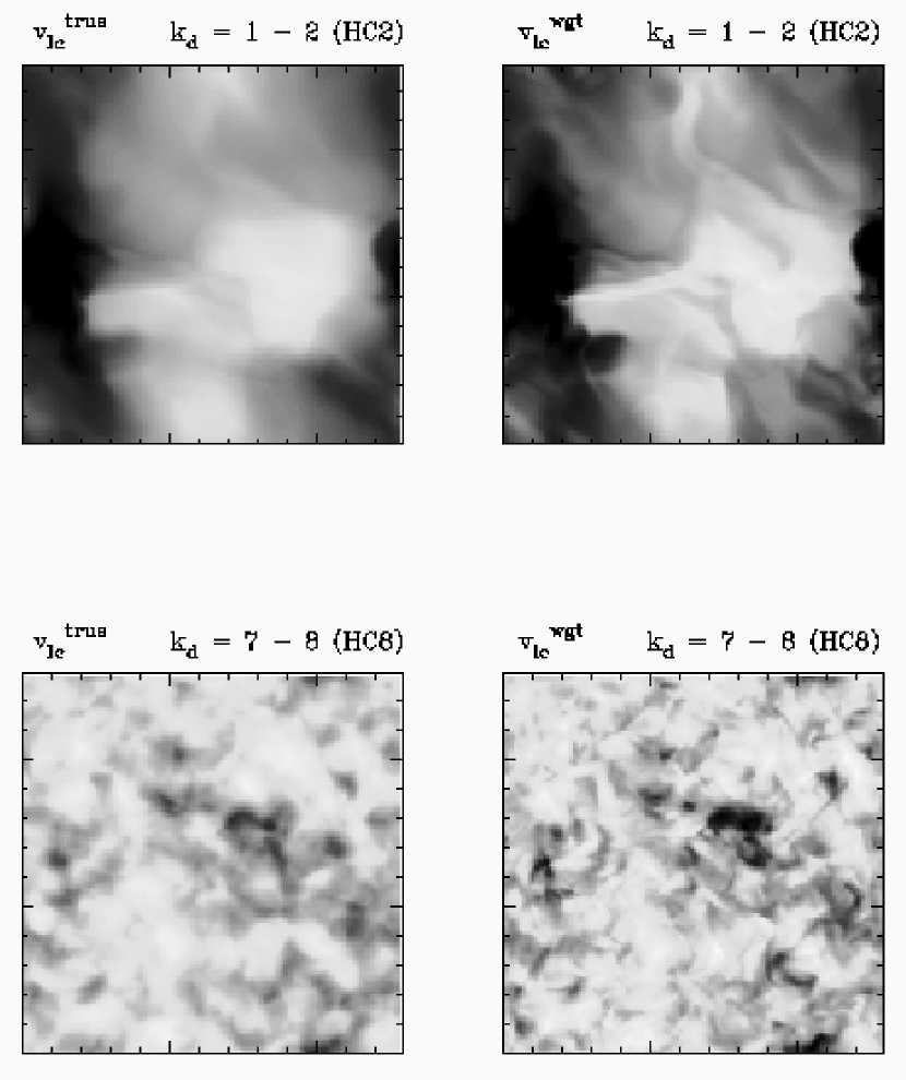
Figure 1: Example velocity line centroid fields obtained from the numerical simulations, for the unweighted case ($v_{lc}^{true}$) and the density weighted case ($v_{lc}^{wgt}$).

First, we examine the driven simulations. Example velocity line centroid fields are shown in Figure 1. It is immediately evident that the inclusion of density-weighting results in the insertion of additional small-scale structure into the line centroid fields.

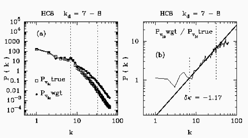
Figure 2: (a) Example velocity line centroid power spectra derived from the numerical simulations (HC8 ; $k_{d}$ = 7–8), for the unweighted case ($P_{v_{lc}^{true}}$) and the density weighted case ($P_{v_{lc}^{wgt}}$). (b) The effect of density weighting determined by the spectral slope, $\delta\kappa$, of $P_{v_{lc}^{wgt}}$$/$$P_{v_{lc}^{true}}$. The dashed lines mark the range of $k$ used for the fit (heavy line) to derive $\delta\kappa$ : from $k$ = 7 (the largest driving scale) to $k$ = 32.

To quantify the effect seen in Figure 1, we calculated the power spectra ($P(k)$ as function of wavenumber $k$) of all the line centroid fields, using a FFT. Figure 2(a) shows representative results for HC8 model ($k_{d}$ = 7–8). There is a turnover in the power spectra at or near $k_{d}$. For $k$ $<$ $k_{d}$, the true and weighted line centroid power spectra are quite similar, while for $k$ $>$ $k_{d}$ the power spectrum of $v_{lc}^{wgt}$ is shallower. We can quantify the effect of density weighting quite precisely by examining the difference (in log space) between the power spectra of $v_{lc}^{wgt}$ and $v_{lc}^{true}$ (in real space this corresponds to measuring the spectral index of the ratio $P_{v_{lc}^{wgt}}$/$P_{v_{lc}^{true}}$). We characterize the ratio of power spectra by a scaling exponent $\delta\kappa$, where : $P_{v_{lc}^{wgt}}$/$P_{v_{lc}^{true}}$ $\propto$ $k^{-\delta\kappa}$ (i.e $log(P_{v_{lc}^{wgt}})$–$log(P_{v_{lc}^{true}})$ = $const$ + $\delta\kappa$ $log(k)$). This procedure avoids potential problems arising from non-power-law projected velocity spectra.

The ratio $P_{v_{lc}^{wgt}}$/$P_{v_{lc}^{true}}$ for the HC8 model is shown in Figure 2(b). There is little modification to the true line centroid power spectrum for spatial scales above the driving scale ($k$ = 7–8); $P_{v_{lc}^{wgt}}$/$P_{v_{lc}^{true}}$ does not vary much with $k$ at small $k$. This is because there are no major density enhancements on these large scales (Ballesteros-Paredes & Mac Low 2002). For $k$ $>$ $k_{d}$, $P_{v_{lc}^{wgt}}$/$P_{v_{lc}^{true}}$ is a well developed power law, with some deviation at very high $k$. We fitted the exponent $\delta\kappa$ = –1.17 $\pm$ 0.06 over the range 7 $\leq$ $k$ $\leq$ 32 (i.e. from the largest driving scale to a wavelength of 4 pixels). The largest scale at which dissipation effects are first seen in these simulations is $\sim$10 zones or $k$ $\approx$ 12.8 (Ossenkopf & Mac Low 2002) but we do not see any spectral breaks in the power spectrum ratio before $k$ = 32; we will examine the effects of this in greater detail in Section 5.2.

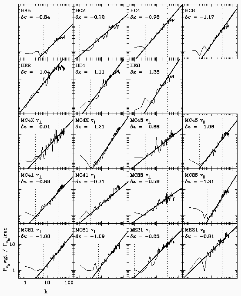
Figure 3: Variation of $P_{v_{lc}^{wgt}}$$/$$P_{v_{lc}^{true}}$ with $k$ for the HD and MHD fields. Fits (heavy lines) to derive $\delta\kappa$ were made in the range of $k$ delimited by the dashed lines (largest driving scale to $k$ = 32).

The other driven models gave similar results. Figure 3 shows $P_{v_{lc}^{wgt}}$/$P_{v_{lc}^{true}}$ for all driven models. These spectra were fitted between the largest driving scale and $k$ = 32 for all models to derive $\delta\kappa$, which in all cases was negative and $\sim$ –1 with variations of up to $\sim$ $\pm$ 0.4. The measured $\delta\kappa$ are listed in Table 1. There is no obvious systematic difference between the HD and MHD cases, nor any obvious variation with rms Mach number, $M$, for the driven runs. There is some evidence that $\delta\kappa$ is more negative when the line of sight is parallel to the mean magnetic field direction, but this does not universally apply. Taking the observed range of $\delta\kappa$ as a natural variation, we derive a mean (unweighted) $\delta\kappa$ = –0.96 $\pm$ 0.22 from all the driven models. In other words, inclusion of density weighting results in a shallower spectral slope, with index $\sim$1 less than the true line centroid power spectrum index. In direct space, such a modification would thus correspond to $\gamma_{2D}$ $\approx$ $\gamma_{3D}$ rather than $\gamma_{2D}$ = $\gamma_{3D}$ + 0.5. (In general, $\gamma_{2D}$ = $\gamma_{3D}$ + 0.5 +$\delta\kappa$/2.)

If the driven turbulence conditions are representative of the conditions within molecular clouds, the scaling exponents measured from line centroid structure functions are approximately equal to the true, 3D exponents. We stress that the “cancellation” of projection smoothing by small scale line centroid structure induced by density inhomogeneity is statistical in nature, and the effect of density weighting does not of course identically reverse the effects of projection smoothing.

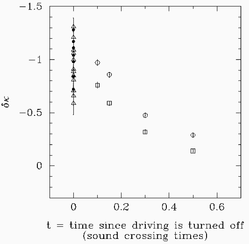
Figure 5: Plot of $\delta\kappa$ versus $t$ = time after driving is turned off in units of the sound crossing time. For the driven runs, we have taken t = 0. Filled circles are driven HD; open triangles are driven MHD; open squares are decaying HD (model D, initial $M$ = 5); open circles are decaying HD (model U, initial $M$ = 50).

The same procedure to derive $\delta\kappa$ was then applied to the simulations of decaying turbulence. Figure 4 shows the plots of $P_{v_{lc}^{wgt}}$/$P_{v_{lc}^{true}}$ evolving as time increases. We have fitted $\delta\kappa$ over the range 10 $\leq$ $k$ $\leq$ 64 for all fields (motivated again by the lack of clear breaks in the power spectrum ratio) and these are listed in Table 1. This shows that as the turbulence decays, the effect of density inhomogeneity on the line centroid field is reduced, due to the lessened density contrast. If molecular clouds are in such a state, then projection smoothing only applies to the observed line centroid field, and $\gamma_{2D}$ $\approx$ $\gamma_{3D}$ + 0.5. Over the course of one sound crossing time, the density contrast is reduced sufficiently, even for initially highly supersonic turbulence, that $\delta\kappa$ becomes very small, due to weaker shocks in decaying turbulence relative to those in driven turbulence (Smith, Mac Low, & Zuev 2000; Smith, Mac Low, & Heitsch 2000); in other words, if the turbulence is continually driven, or has only recently entered a decaying state, then we expect $\delta\kappa$ $\approx$ –1, but this evolves quickly to $\delta\kappa$ $\longrightarrow$ 0 over a sound crossing time. Figure 5 summarizes the evolution of $\delta\kappa$ after the driving is turned off.

5.2 Regime of Validity 

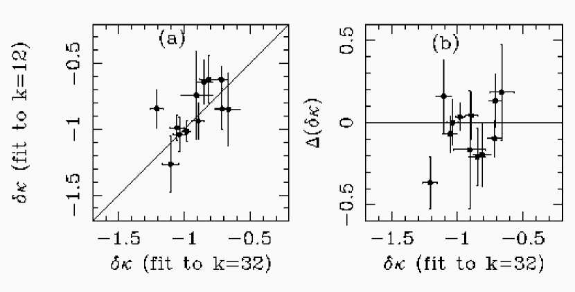
Figure 6: a) Plot of $\delta\kappa$ derived from fits to the power spectrum ratio fitted up to $k$ = 12 versus $\delta\kappa$ derived from fits to the power spectrum ratio fitted up to $k$ = 32, for a subset of the driven runs (see text). The solid line is a line of equality. (b) Difference between the $\delta\kappa$ values shown in (fit to $k$ = 32 minus fit to $k$ = 12). The solid line marks a difference of zero.

As noted above, we are fitting $\delta\kappa$ over a range of $k$ that includes the dissipation region ($k$ greater than $\sim$ 12.8), motivated by the lack of distinct breaks in the power spectrum ratio. To test whether dissipative effects could induce systematic biases in our results, we repeated the fits while restricting the range to a maximum $k$ = 12. This was done only for the driven models for which $k_{d}$ = 1–2 and $k_{d}$ = 3–4 in order that sufficient data was still available for the fits. The resulting measurements of $\delta\kappa$ are plotted against the measurements of $\delta\kappa$ fitted to $k$ = 32 in Figure 6. For this sample, we find that the mean $\delta\kappa$ are –0.91 $\pm$ 0.17 (fitted to $k$ = 32) and –0.87 $\pm$ 0.19 (fitted to $k$ = 12). These are not significantly different, so our visual conclusion that there are no breaks in the power spectrum ratios is good.

The advantage of using a relative measure, $\delta\kappa$, in the above analysis is that it circumvents potential problems arising from small curvatures in the intrinsic velocity power spectra. We now examine actual measurements of the spectral indices of the projected velocity power spectra. These absolute indices are needed to examine the range of validity of $\delta\kappa$ as derived above. Due to the curvature in the power spectra, likely arising from dissipative effects at higher $k$, the absolute spectral slopes depend on the range in $k$ over which they are derived. In what follows, we label the spectral slope of the unweighted projected velocity field as $\kappa_{2D,u}$ and the spectral slope of the density-weighted projected velocity field as $\kappa_{2D,w}$. These are related by $\kappa_{2D,w}$ –$\kappa_{2D,u}$ = $\delta\kappa$.

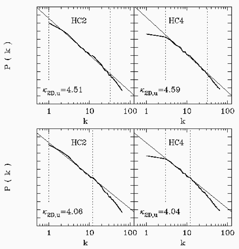
Figure 7: Velocity line centroid power spectra for models HC2 and HC4. The dotted lines delimit the range of $k$ used in the power law fits (straight lines) to $\kappa_{2D,u}$.

Example line centroid power spectra for the HC2, HC4 models, driven at $k_{d}$ = 1–2 and 3–4 respectively, are shown in Figure 7. These are fitted over two ranges in $k$: up to $k$ = 32 (upper panels) and up to $k$ = 12 (lower panels); in both cases the smallest $k$ used to make the fit is taken as the smaller of the driving wavenumbers. When the fit is made to $k$ = 32, the spectra are “steep” ($\kappa_{2D,u}$ $\sim$ 4.5) but when the fit is made to $k$ = 12, the indices are in good agreement with the value expected for Burgers turbulence ($\kappa_{2D,u}$ $\sim$ 4). Numerical dissipation will cause just the sort of steepening of the spectrum (less structure at small scale) that is seen in Figure 7.

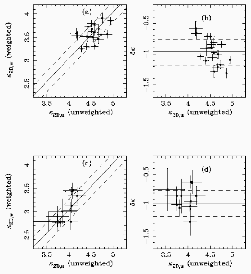
Figure 8: (a) Plot of the density-weighted velocity line centroid spectral index, $\kappa_{2D,w}$, versus the unweighted (true) velocity line centroid spectral index, $\kappa_{2D,u}$ for all driven runs, with the indices fitted to $k$ = 32. (b) Plot of $\delta\kappa$ (= $\kappa_{2D,w}$–$\kappa_{2D,u}$) versus $\kappa_{2D,u}$ for all driven runs, with the indices fitted to $k$ = 32. (c) Plot of the density-weighted velocity line centroid spectral index, $\kappa_{2D,w}$, versus the unweighted (true) velocity line centroid spectral index, $\kappa_{2D,u}$ for a subset of the driven runs (see text), with the indices fitted to $k$ = 12. (b) Plot of $\delta\kappa$ (= $\kappa_{2D,w}$–$\kappa_{2D,u}$) versus $\kappa_{2D,u}$ for a subset of the driven runs (see text), with the indices fitted to $k$ = 12. In all plots the solid line denotes the relationship $\delta\kappa$ = –0.96 and the dashed lines mark uncertainties of $\pm$ 0.22 around this relationship.

We have derived $\kappa_{2D,u}$, $\kappa_{2D,w}$ and $\delta\kappa$ for the driven runs over the two ranges in $k$ given above. Figure 8(a) shows the relation between $\kappa_{2D,u}$ and $\kappa_{2D,w}$ for all driven runs fitted to $k$ = 32; the corresponding variation of $\delta\kappa$ with $\kappa_{2D,u}$ is shown in Figure 8(b). Figures 8(c) and  8(d) show the same relations obtained when the fits are made to $k$ = 12 for the subset of runs with $k_{d}$ = 1–2 and $k_{d}$ = 3–4. In all these Figures, the solid line denotes $\delta\kappa$ = –0.96 derived in the preceding Section, and the dashed lines mark uncertainties of $\pm$0.22 around this value.

These tests show that our estimated mean $\delta\kappa$ = –0.96 $\pm$ 0.22 is not strongly affected by the fitting range in $k$ but there is some uncertainty in the absolute range of $\kappa_{2D,u}$ and $\kappa_{2D,w}$ to which this value applies. Conservatively, the fits to $k$ = 12 should be used, as these are free of dissipative effects. Using only the fields for which such fits can be made, we find that $\delta\kappa$ = –0.87 $\pm$ 0.19, and this applies to $\kappa_{2D,u}$ $\approx$ 3.5–4.2 and $\kappa_{2D,w}$ $\approx$ 2.7–3.4.

However, we also note that the lack of dependence of $\delta\kappa$ on the fitting range in $k$ is indirect evidence that a single value of $\delta\kappa$ is applicable at all $\kappa_{2D,u}$, but this interpretation should be examined in more detail in future. In what follows we shall assume that $\delta\kappa$ = –0.96 $\pm$ 0.22 holds for all $\kappa_{2D,u}$ and $\kappa_{2D,w}$.

5.3 Origin of the Spectral Modification

5.3.1 Effect of Density Spectral Index

Lazarian & Esquivel (2003) have suggested that (in our terminology) $\delta\kappa$ may have a larger amplitude for “shallow” density field power spectra. The density field power spectrum slope may be estimated from the power spectrum of the projected column density field, $P_{cd}(k)$, using the same arguments as presented in § 2 (see also Lazarian & Pogosyan 2000; Stutzki et al. 1998). If $\delta\kappa$ is related to the spectral slope, $\kappa_{cd}$, of the column density power spectrum (where $P_{cd}(k)$ $\propto$ $k^{-\kappa_{cd}}$) then this would indeed provide a means of inferring $\delta\kappa$ observationally. In other words, the observed column density power spectrum slope is used as a probe of the (relative) density fluctuation spectrum as a function of scale within the medium.

To investigate this, we produced column density maps for all the simulations (including projection along two axes – parallel and perpendicular to the magnetic field – for the MHD fields). We then fitted $\kappa_{cd}$ for each field, using the same range in wavenumber that was used to derive $\delta\kappa$. The fitted values of $\kappa_{cd}$ are given in Table 1. (The column density power spectra are also slightly curved, so $\kappa_{cd}$ would be lower if fitted to $k$ = 12; thus the $\kappa_{cd}$ axis is uncertain by a $\sim$linear shift as in Figure 8 for $\kappa_{2D,u}$.)

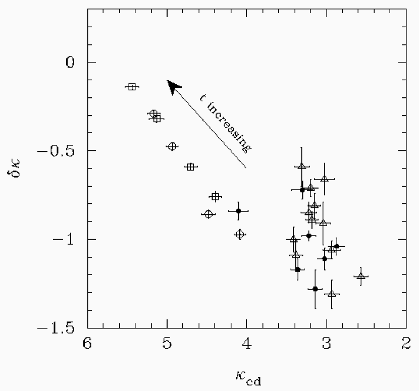
Figure 9: Plot of $\delta\kappa$ versus $\kappa_{cd}$ for all simulations. Filled circles are driven HD; open triangles are driven MHD; open squares are decaying HD (model D, initial $M$ = 5); open circles are decaying HD (model U, initial $M$ = 50). The arrow shows the direction of evolution of $\delta\kappa$ as time (since driving is turned off) increases; see Figure 5.

In Figure 9 we plot the variation of $\delta\kappa$ with $\kappa_{cd}$. There is a clear variation of $\delta\kappa$ with $\kappa_{cd}$, demonstrated by the decaying turbulence simulations. As time proceeds, $\kappa_{cd}$ increases (i.e. preferential reduction in small scale density contrast) and the amplitude of $\delta\kappa$ diminishes (i.e. lessened effect of density inhomogeneity on the velocity line centroid field). For the driven simulations, the $\kappa_{cd}$ are typically $\sim$ 3. These are in reasonable accord with observational estimates of $\kappa_{cd}$ $\approx$ 2.8 for molecular clouds; e.g. Bensch, Stutzki, & Ossenkopf 2001. For our $\kappa_{cd}$ $\sim$ 3, $\delta\kappa$ varies around the mean value of –1. Thus, observational estimates of $\kappa_{cd}$ suggest that accounting for density inhomogeneity is very important for velocity line centroid analysis of molecular clouds, implying (with $\delta\kappa$ $\approx$ –1) that $\gamma_{2D}$ $\approx$ $\gamma_{3D}$ counter to the expectations based on projection smoothing alone. This provides an explanation for the $\gamma_{2D}$ $\approx$ $\gamma_{3D}$ result observed in these simulations by Ossenkopf & Mac Low (2002). Lazarian & Pogosyan do not provide a physical motivation for whether the medium is density dominated (i.e. “shallow density spectrum” having $\kappa_{cd}$ $\leq$ 3) or not: it is simply a question of what $\kappa_{cd}$ is, regardless of why. In our scenario, this regime is the driven turbulence regime.

5.3.2 Amplitude of Density Fluctuations

A note of caution regarding the use of $\kappa_{cd}$ to infer $\delta\kappa$ should be made: $\kappa_{cd}$ is a non-unique measure of the density field. To investigate this more deeply, we analyzed modified versions of the HE2 field. First, we randomized the Fourier space phases of the density and velocity fields to produce new fields with the same power spectra as the original fields. This modification has two effects : (1) it removes the density-velocity correlations, (2) it drastically reduces the amplitude of density fluctuations. Following phase-randomization of the density field, we found that we had to recenter the mean density due to the creation of negative densities by the phase-randomization process. After renormalization back to a mean density of unity, the phase-randomized density field had a standard deviation of 0.21 and range of 1$\times$10^-6 to 2.02. For comparison, the original density field, normalized to mean unity, had a standard deviation of 2.53 and a range of 1.2$\times$10^-6 to 92.1. The logarithm of the phase-randomized density field had a standard deviation of 0.22, compared to the standard deviation of the logarithm of the original density field of 2.49. Using the phase-randomized density fields and velocity fields we derived $\delta\kappa$ = –0.18 $\pm$ 0.03. This is substantially lower than the original $\delta\kappa$ = –1.04 $\pm$ 0.05 obtained with the original HE2 density and velocity fields. This shows that the “shallowness” of the density power spectrum, as measured by $\kappa_{cd}$, does not uniquely allow inference of $\delta\kappa$.

We conducted a second test, this time randomizing the phases of the logarithm of density, and then exponentiating the phase-randomized log(density) field. This procedure again removes the density-velocity correlations but does not lead to the creation of negative densities, and allows a greater amplitude of density contrast. We found that the resulting $\kappa_{cd}$ $\approx$ 2.41 for the density field produced by this method was slightly shallower than the original $\kappa_{cd}$ $\approx$ 2.87 for the HE2 model. The standard deviation of log(density) was the same for the phase-randomized density field and the original density field (2.49). Using the exponentiated phase-randomized log(density) field in conjunction with the phase-randomized velocity field, we found $\delta\kappa$ = –1.16 $\pm$ 0.05.

These two tests together suggest that it is the amplitude of density fluctuations, measured as the standard deviation of log(density) that is controlling the value of $\delta\kappa$. To make sure that this is the case, and that density-velocity correlation does not play a major role, we took the original velocity field and the original density field, shifted by 64 pixels from its original position. For a shift along the line-of-sight, we derived $\delta\kappa$ = –0.90 $\pm$ 0.04 and for a shift transverse to the line-of-sight we derived $\delta\kappa$ = –0.97 $\pm$ 0.06. These are slightly lower in magnitude than the original $\delta\kappa$ = –1.04 $\pm$ 0.05, but the difference is marginally significant.

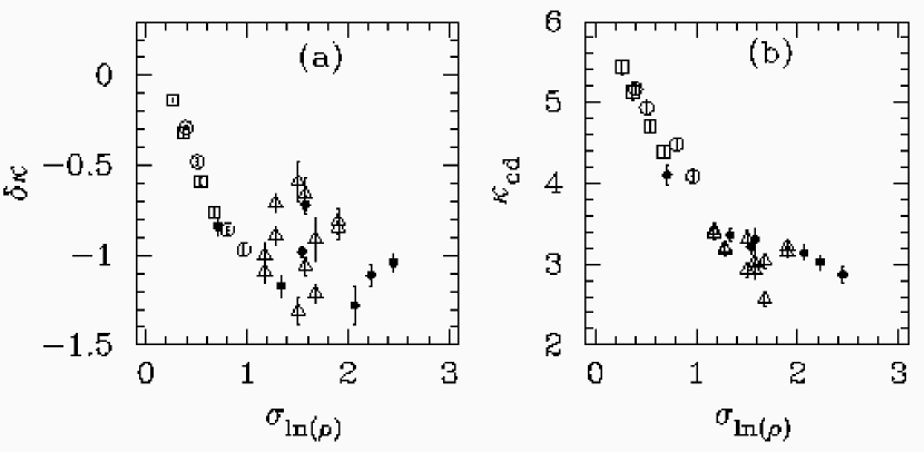
Figure 10: (a) Plot of $\delta\kappa$ versus $\sigma_{ln(\rho)}$ for all simulations. (b) Plot of $\kappa_{cd}$ versus $\sigma_{ln(\rho)}$ for all simulations. Filled circles are driven HD; open triangles are driven MHD; open squares are decaying HD (model D, initial $M$ = 5); open circles are decaying HD (model U, initial $M$ = 50). The phase-randomized density model has $\sigma_{ln(\rho)}$ = 0.22, $\delta\kappa$ = –0.18, $\kappa_{cd}$ = 2.87.

We thus conclude that the amplitude of density contrast is most important in determining $\delta\kappa$. To examine this directly, we measured the standard deviation of log(density), $\sigma_{ln(\rho)}$, for all the numerical fields (see Table 1) and we plotted this versus $\delta\kappa$ (Figure 10(a)) and against $\kappa_{cd}$ Figure 10(b)). This indicates that there is a fairly good correlation between $\delta\kappa$ and $\sigma_{ln(\rho)}$, and that with the assumption that the numerical fields are a better representation of real molecular clouds than the phase-randomized fields, that $\kappa_{cd}$ may be used as a surrogate for $\sigma_{ln(\rho)}$. We find that the driven simulations are characterized by $\kappa_{cd}$ $\approx$ 3 and $\sigma_{ln(\rho)}$ exceeding $\sim$ unity, but that there is no obvious dependence of $\delta\kappa$ on $\kappa_{cd}$ or $\sigma_{ln(\rho)}$ within this regime.

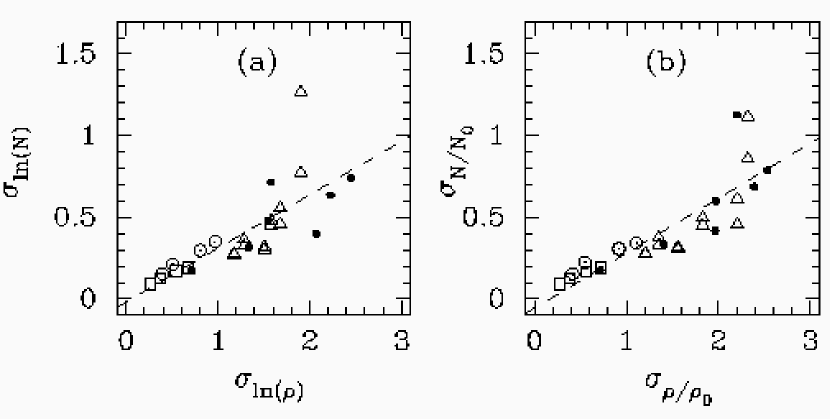
Figure 11: (a)Plot of $\sigma_{ln(N)}$ versus $\sigma_{ln(\rho)}$ for all simulations. (b) Plot of $\sigma_{N/N_{0}}$ versus $\sigma_{\rho/\rho_{0}}$ for all simulations. Filled circles are driven HD; open triangles are driven MHD; open squares are decaying HD (model D, initial $M$ = 5); open circles are decaying HD (model U, initial $M$ = 50).

Ideally, one would like to measure $\sigma_{ln(\rho)}$ to infer $\delta\kappa$ but it is of course impossible to measure $\sigma_{ln(\rho)}$ directly. However, it may be possible to infer $\sigma_{ln(\rho)}$ indirectly using the column density field. Figure 11(a) compares the variation in the standard deviation of log(column density), $\sigma_{ln(N)}$, to $\sigma_{ln(\rho)}$. The dashed line is fitted : $\sigma_{ln(N)}$ = –0.02 $\pm$ 0.08 + (0.33 $\pm$ 0.06)$\sigma_{ln(\rho)}$ as a guide. The values of $\sigma_{ln(N)}$ are listed in Table 1. Unfortunately, it is also impossible to use $\sigma_{ln(N)}$ observationally, as the small $N$ are dominated by noise. Instead, we consider simply the standard deviation of density, $\sigma_{\rho/\rho_{0}}$, and column density $\sigma_{N/N_{0}}$, where both fields are normalized their mean values, $\rho_{0}$ and $N_{0}$, respectively. The dependence of $\sigma_{N/N_{0}}$ on $\sigma_{\rho/\rho_{0}}$ is shown in Figure 11(b) along with the fitted line, $\sigma_{N/N_{0}}$ = –0.06 $\pm$ 0.07 + (0.34 $\pm$ 0.04)$\sigma_{\rho/\rho_{0}}$. These results show that the variation in column density may be used to infer the variation in (3D) density, but the dynamic range in $N$ is compressed due to line-of-sight averaging ($\sigma_{N/N_{0}}$ $\approx$ $\sigma_{\rho/\rho_{0}}$/3). However, in general, it should be recognized that, at any finite resolution, the mean density and column density are well-estimated, but their standard deviations are continuously variable with resolution in the respective dimensions. It may be possible to attempt to construct a resolution-independent measure to compare 2D and 3D standard deviation but this is beyond the scope of the current work.

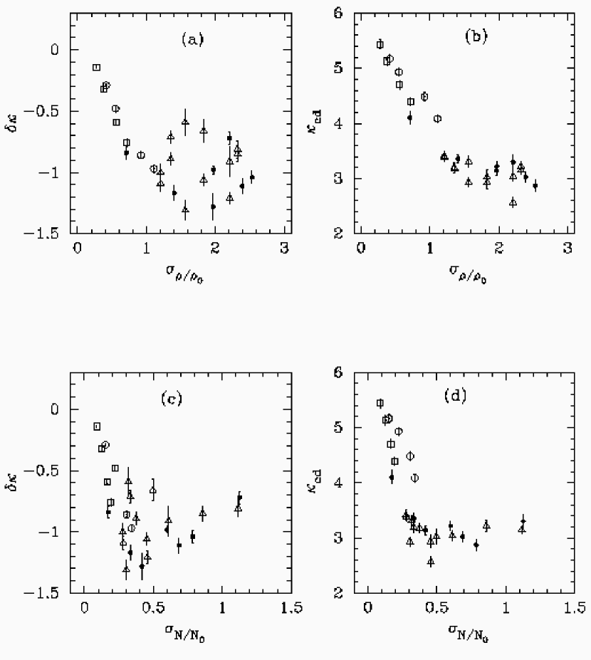
Figure 12: (a) Plot of $\delta\kappa$ versus $\sigma_{\rho/\rho_{0}}$ for all simulations. (b) Plot of $\kappa_{cd}$ versus $\sigma_{\rho/\rho_{0}}$ for all simulations. (c) Plot of $\delta\kappa$ versus $\sigma_{N/N_{0}}$ for all simulations. (d) Plot of $\kappa_{cd}$ versus $\sigma_{N/N_{0}}$ for all simulations. Filled circles are driven HD; open triangles are driven MHD; open squares are decaying HD (model D, initial $M$ = 5); open circles are decaying HD (model U, initial $M$ = 50). The phase-randomized model has $\sigma_{\rho/\rho_{0}}$ = 0.21, $\sigma_{N/N_{0}}$ = 0.065, $\delta\kappa$ = –0.18, and $\kappa_{cd}$ = 2.87.

In Figure 12 we plot combinations of $\sigma_{\rho/\rho_{0}}$, $\sigma_{N/N_{0}}$, $\delta\kappa$, and $\kappa_{cd}$ to gauge the utility of different measures. In summary, some guidelines concerning $\delta\kappa$ may be established observationally by measuring $\kappa_{cd}$ and $\sigma_{N/N_{0}}$. Note that a measurement of $\kappa_{cd}$ and $\sigma_{N/N_{0}}$ may also be used to distinguish the phase-randomized fields from the numerically simulated fields : the phase-randomized density field has a much lower $\sigma_{N/N_{0}}$ = 0.065 compared with that of the numerical field ($\sigma_{N/N_{0}}$ = 0.786) for the same $\kappa_{cd}$ = 2.87. Some caution comparing $\sigma_{N/N_{0}}$ with Figure 12 is needed if the observations are at significantly different spatial dynamic range than the simulations used here.

5.4 Comparison with Previous Results

Our results appear inconsistent with two previous studies. Brunt et al. (2003) found that $\delta\kappa$ $\approx$ –0.4 from the simulation used in their paper (Mach number $\approx$ 1). The density field used in Brunt et al. (2003) had $\sigma_{ln(\rho)}$ = 0.45. Comparison with Figure 10(a) shows that these numbers are not discrepant with the current results. The conclusion of Brunt et al. (2003) that, for a given amplitude of density fluctuations, the correlations between density and velocity are important was based on the a single simulation and is outweighed by our new results here. Secondly, our results are inconsistent with the results ($\delta\kappa$ $\approx$ 0) found by Lazarian & Esquivel (2003) for their simulation (Mach number $\approx$ 2.5). This may be due to the solenoidal driving in their simulations (Cho & Lazarian 2002); certainly this discrepancy deserves further attention.

5.5 Resolution Tests

Finally, we examined the effect of limited spatial dynamic range on our results. The driven numerical fields implicitly contain realizations at different effective resolutions (i.e. due to the varying driving scales). These show no obvious trend of $\delta\kappa$ with driving wavelength; however there is a large amount of scatter in the derived $\delta\kappa$ that may hide such a trend. In addition we have explored the effect of limiting the fits to $\delta\kappa$ to different ranges of $k$. We conducted a further, more direct, tests using realizations of model D (decaying turbulence) at sizes of 128³ and 64³ and a realization of model HC2 (driven turbulence) at 256³ resolution. These realizations utilize the same parameterization but are not identical in detail (i.e. they were not initialized with the same random number seeds and so are subject to the natural scatter in $\delta\kappa$ evidenced in Table 1).

Snapshots of model D at 128³ and 64³ sizes are available at timesteps of 0.1, 0.15 and 0.3 sound crossing times. We conducted the same analysis to derive $\delta\kappa$ from these lowered resolution simulations. At 128³ size, we find $\delta\kappa$ = –0.78 $\pm$ 0.08, –0.57 $\pm$ 0.04 , and –0.22 $\pm$ 0.03 for times 0.1, 0.15 and 0.3 respectively. At 64³ size, we find $\delta\kappa$ = –0.71 $\pm$ 0.21, –0.33 $\pm$ 0.22 , and –0.11 $\pm$ 0.25 for times 0.1, 0.15 and 0.3 respectively As the resolution is increased, the $\delta\kappa$ are converging to the values of $\delta\kappa$ $=$–0.76 $\pm$ 0.03,–0.59 $\pm$ 0.02, and –0.32 $\pm$ 0.02 found at 256³ size at the same timesteps. The driven model HC2, with higher Mach number, showed a somewhat more pronounced shift, from $\delta\kappa$ $=$ –0.72 $\pm$ 0.05 at 128³ to $\delta\kappa$ $=$ –1.01 $\pm$ 0.03 at 256³. In sum, this resolution study suggests that the magnitude of $\delta\kappa$ is decreased slightly by limited spatial dynamic range. Therefore, our derived $\delta\kappa$ magnitudes should probably be considered to be lower limits (i.e. the true, high resolution, values may be a little more negative than found here).

6 Velocity Line Centroid Analysis : Observational Results

6.1 Overview

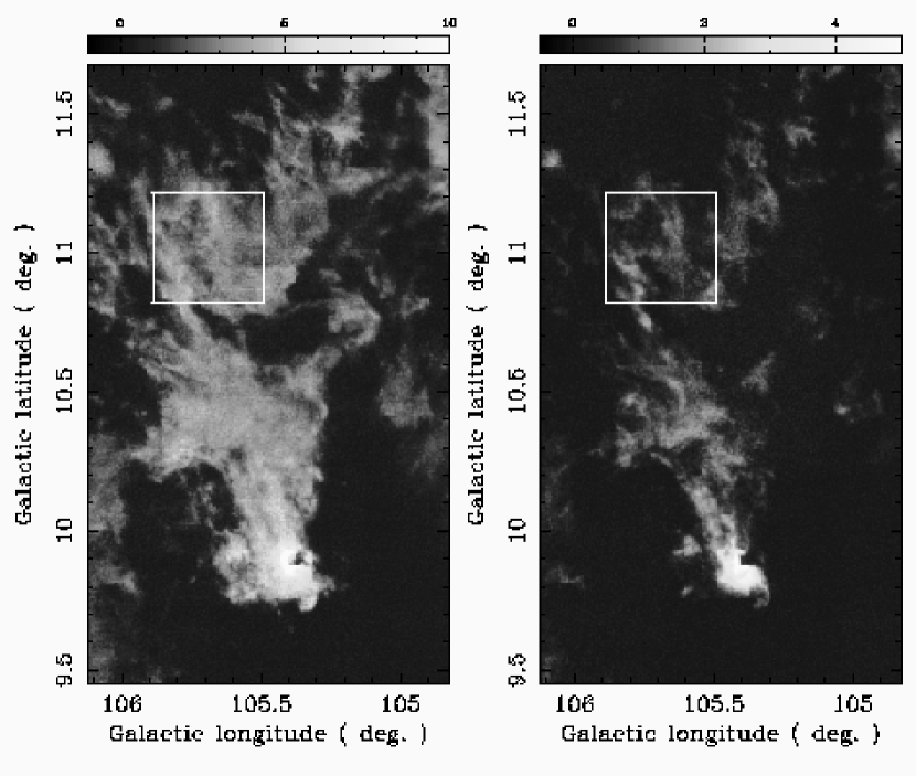
Figure 13: Overview of the region near NGC 7129 selected for velocity line centroid analysis. Left : ¹²CO peak temperature image. Right : ¹³CO peak temperature image. The wedges show antenna temperature in K.

An overview of the CGPS CO data in the vicinity of NGC 7129 is given in Figure 13. We have selected a region (64 $\times$ 64 pixels, 32 $\times$ 32 beams, 4096 spectra) for velocity line centroid analysis, indicated by the superimposed square in Figure 13. This region is located away from the main star forming area (it contains no IRAS point sources), and has simple, singly-peaked spectral lines. To derive velocity line centroid maps, we utilized Gaussian fitting to the spectral lines rather than a direct projection via Equation 4, as Gaussian fitting was found to be less noisy (see below). Example fits to both the ¹²CO lines and ¹³CO lines are shown in Figure 14. These spectra are taken from a 16 $\times$ 16 pixel block at the center of the analysis region and are block-averaged over 4 $\times$ 4 pixels. The ¹²CO lines have roughly twice the peak temperature of the ¹³CO lines, resulting in comparable signal-to-noise for each tracer.

Fits to the ¹³CO lines could not be made for the entirety of the analysis region, due to weak or absent emission. Use of the ¹³CO line centroid field for analysis would then require values for the missing data to be assumed before calculation of the power spectrum. A possible choice would be to set the missing data to the mean value of the measurable data. However, a better procedure is to create a “hybrid” line centroid field, using the ¹²CO centroid velocities as the best estimate of the missing ¹³CO centroid velocities. We thus masked off all pixels in the analysis region for which the peak temperature of the ¹³CO line was less than 1.4 K $T_{A}^{*}$ (i.e. $\sim$ 5$\sigma$), and replaced the absent or noisy ¹³CO measurements with the ¹²CO centroid velocities. For the hybrid field, 40% of the line centroid velocities are from ¹³CO and 60% are from ¹²CO.

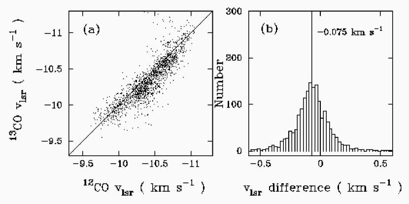
Figure 15: (a) Comparison of the velocity line centroids derived from ¹²CO and ¹³CO where both measurements can be made. (b) Histogram of the differences in measured $v_{lsr}$ (¹²CO velocity minus ¹³CO velocity).

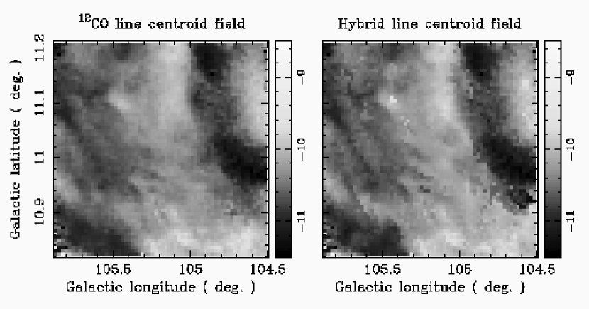
Figure 16: The observed velocity line centroid maps.

For the lines of sight where we have good fits to both ¹³CO and ¹²CO, we compared the derived line centroid velocities, as shown in Figure 15(a). The two measurements are very similar over the entire variation of centroid velocity ($\sim$ –11 to –9.5 km s^-1) but there is a slight average offset between the two, of –0.075 km s^-1 ($\sim$ 1/2 channel width) as seen in Figure 15(b). This can arise from greater saturation on one side of the ¹²CO line profiles, or from depth-dependent abundance variations in the presence of a line-of-sight velocity gradient. The effects of opacity on our measured ¹²CO velocity line centroid map are thus very small. With the offset understood, the width of the distribution in Figure 15(b) ($\sim$ $\pm$ 0.1 km s^-1) can be otherwise attributed to noise on the measurements. To measure the noise on the line centroid fields, we took the fitted Gaussian line profiles as the best estimate of the true line profiles and added actual instrumental noise from the same spatial positions, taken from a signal-free area of the baseline region. We then carried out the same Gaussian fitting procedure to derive the noise distribution. For comparison, we derived the direct line centroid field from the “re-noised” fields using Equation 4. The estimated errors on the ¹²CO line centroid field are $\pm$ 0.093 km s^-1 (Gaussian fitting) and $\pm$ 0.122 km s^-1 (using Equation 4). The Gaussian-fitting procedure is less noisy, and as the lines in the original data are well-described by Gaussians (Figure 14), we used the line centroids derived by Gaussian fitting for the power spectrum analysis below. The resulting velocity line centroid fields derived from Gaussian fitting are shown in Figure 16. The observed fields are qualitatively more similar to the simulations driven at large scale (the $k_{d}$ = 1-2 case in Figure 1) than to those driven at small scale.

6.2 Large Scale Gradients and Edge Effects

Prior to the full analysis, we investigated the effect of filtering out the “large-scale” line centroid velocity fluctuations. Whether this should be done or not is a matter of some controversy (Miesch & Bally 1994; Ossenkopf & Mac Low 2002). We estimated the large-scale gradients by fitting a quadratic surface to the ¹²CO line centroid map. Then we subtracted this from the original line centroid map, and calculated the power spectrum before and after subtraction, using FFTs. We found that only the low frequency ($k$ = 1) power is strongly affected by this procedure, as may have been expected. The measured spectral slopes, between $k$ = 2 and $k$ = 13 (see below) are $\kappa_{2D}$ = 3.38 $\pm$ 0.10 (before subtraction) and $\kappa_{2D}$ = 3.42 $\pm$ 0.09 (after subtraction). Thus the spectrum steepens slightly (but insignificantly) after subtraction of the large-scale gradients, most likely due to the suppression of high frequency structure resulting from mismatch in the line centroids at the field edges (i.e. the FFT routine assumes periodic fields). As there is little difference between the line centroid power spectrum before and after subtraction of the large-scale gradients, and it is not clear whether they should be subtracted, we do not employ the subtraction in the analysis below.

We also examined the effect of apodization (Miville-Deschênes, Lagache & Puget 2002). We centered the ¹²CO line centroid field to zero mean, then applied a cosine taper to a strip 2 pixels wide around the edge of the field. The edges of the line centroid field now match at zero velocity. For the apodized field, we applied the same taper function to the noise estimates, to ensure that the noise floor is still well estimated. At large $k$ both the apodized line centroid power spectrum and the apodized noise floor are reduced, resulting in comparable signal-to-noise before and after apodization. After subtraction of the respective noise floors (see below) the fitted spectral slopes are $\kappa_{2D}$ = 3.70 $\pm$ 0.13 (before apodization) and $\kappa_{2D}$ = 3.76 $\pm$ 0.12 (after apodization). There is little to distinguish these measurements over the measurement uncertainty, so we do not utilize apodization in the analysis below. As the apodization routine simply imposes arbitrary smooth structure in the line centroid field, it is not surprising that the measured power spectrum slope steepens slightly (i.e. reduction of small scale power). Alternatively, the untapered field contains unphysical sharp velocity structure at the field edges, so the actual noise-floor subtracted spectral slope most likely lies between the two slope estimates above.

6.3 Correction for Noise and Beam Smearing

The raw measured indices stated above ($\kappa_{2D}$ $\approx$ 3.4) are not the actual true measured indices, as we have not yet accounted for the effects of measurement noise and beam smearing on the measured power spectra. The total power spectrum in the presence of noise is, simply, $P_{true}(k)$ + $P_{noise}(k)$ (where $P_{true}$ is the power spectrum that would be observed in the absence of noise) assuming independence of the signal and noise. The noise power spectrum must thus be subtracted from the raw measured power spectrum prior to analysis. The finite size of the telescope beam induces correlations between closely spaced pixels; for a beam pattern $B(x,y)$ in direct space (i.e. roughly a Gaussian form with 45″ FWHM), the observed line centroid map (neglecting noise for now) is : $v_{lc}^{obs}$ = $v_{lc}^{obs,true}$ $\otimes$ $B$ where $\otimes$ denotes convolution and $v_{lc}^{obs,true}$ is the line centroid field that would be observed without beam smearing. The beam smeared power spectrum is then $P_{v_{lc}^{obs}}(k)$ = $P_{v_{lc}^{obs,true}}(k)$$P_{B}(k)$ where $P_{B}(k)$ is the power spectrum of the beam pattern. The final output power spectrum, corrected for noise and beam smearing is:

$$P_{output}(k)\;\;\;=\;\;\;(P_{v_{lc}^{obs}}(k)\;-\;P_{noise}(k))\;/\;P_{B}(k).\;\;$$

Note that the division out of the beam pattern is applied after the noise floor subtraction as the noises in our data are spatially independent (in contrast to the measured signal).

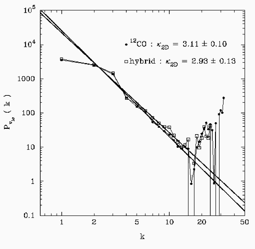
Figure 18: Output velocity line centroid power spectra after noise floor subtraction and beam pattern division (Equation 5). The heavy lines are the fits of $\kappa_{2D}$ to these spectra in the range $k$ = 2 to $k$ = 13.

The noise power spectra can be derived from the “re-noised” fields discussed above; we did this for both the ¹²CO line centroid field and the hybrid line centroid field. We assumed that a Gaussian beam pattern, $B(x,y)$ of 45″ FWHM applied to both the ¹²CO line centroid field and the hybrid line centroid field. A summary of the relevant terms in Equation 5 is provided in Figure 17. Output power spectra were then derived via Equation 5 and these are shown in Figure 18. The resulting scaling range covers $k$ = 2 to $k$ = 13 limited at low $k$ by a possible turnover and the uncertainty of large-scale gradient subtraction, and limited at high $k$ by the amplification of measurement noise by beam pattern division. The resulting fits to the range $k$ = 2 to $k$ = 13 are $\kappa_{2D}$ = 3.11 $\pm$ 0.10 and $\kappa_{2D}$ = 2.93 $\pm$ 0.13 for the ¹²CO line centroid field and the hybrid line centroid field respectively. These are jointly consistent with $\kappa_{2D}$ $\approx$ 3, giving $\gamma_{2D}$ $\approx$ 0.5.

The range of the fit appears deceptively large in Figure 18; the spatial dynamic range achieved is only 6.5, between wavelengths of 32 and 4.9 spatial pixels ($\sim$2.5 beamwidths). Similar spatial dynamic range was achieved by Miesch & Bally (1994), who measured a typical value of $\gamma_{2D}$ $\approx$ 0.43. Around three orders of magnitude in spatial dynamic range was achieved for the Polaris Flare molecular cloud by Ossenkopf & Mac Low (2002) by combining three data sets at different angular resolutions and spatial scales; they also measured $\gamma_{2D}$ $\approx$ 0.5.

6.4 Interpretation

If we interpret the measured index of $\kappa_{2D}$ $\approx$ 3 ($\gamma_{2D}$ $\approx$ 0.5) allowing for projection smoothing but without taking into account the effect of density weighting then the inferred 3D spectral index is $\kappa_{3D}$ $\approx$ 3. We would thus obtain $\gamma_{3D}$ $\approx$ 0 (via Equation 2) or : no dependence of “turbulent” velocity dispersion on scale. If correction for projection smoothing is applied to the indices measured by Miesch & Bally (1994) and Ossenkopf & Mac Low (2002), this again gives $\gamma_{3D}$ $\approx$ 0. A similar result (i.e. $\gamma_{3D}$ $\approx$ 0) was found by O’Dell & Castaneda (1987) for H II region turbulence, after correcting for projection smoothing. The correction for projection smoothing, however, has been the exception rather than the rule for velocity line centroid analysis and most authors have taken their projected $\gamma_{2D}$ as being equivalent to the intrinsic $\gamma_{3D}$. This is not correct, as the selection of the $k_{z}$ = 0 plane of the 3D line of sight velocity power spectrum by projection onto the 2D plane of the sky is purely a geometrical effect : projection smoothing thus always applies (unless the cloud is actually two dimensional – see below), being modified only by the effects of density inhomogeneity (and radiative transfer). Hobson (1992) interprets (e.g.) $\kappa_{2D}$ = 3 (i.e. $\gamma_{2D}$ = 0.5) as being applicable to shock-dominated turbulence ($\gamma_{3D}$ = 0.5). Miesch & Bally (1994) directly compare their $\gamma_{2D}$ to theoretical predictions of $\gamma_{3D}$ with no modification. Lazarian & Esquivel (2003) derive from their numerical data (in our terminology) $\delta\kappa$ = 0, but then interpret the $\gamma_{2D}$ $\approx$ 0.43 of Miesch & Bally (1994) as meaning also that $\gamma_{3D}$ $\approx$ 0.43.

Our numerical results here show that the (statistical) equivalence of $\gamma_{2D}$ and $\gamma_{3D}$ is actually valid in the case of driven turbulence but only due to the accidental cancellation of two competing factors : projection smoothing, which suppresses small scale velocity line centroid structure, and density inhomogeneity, which creates small scale velocity line centroid structure.

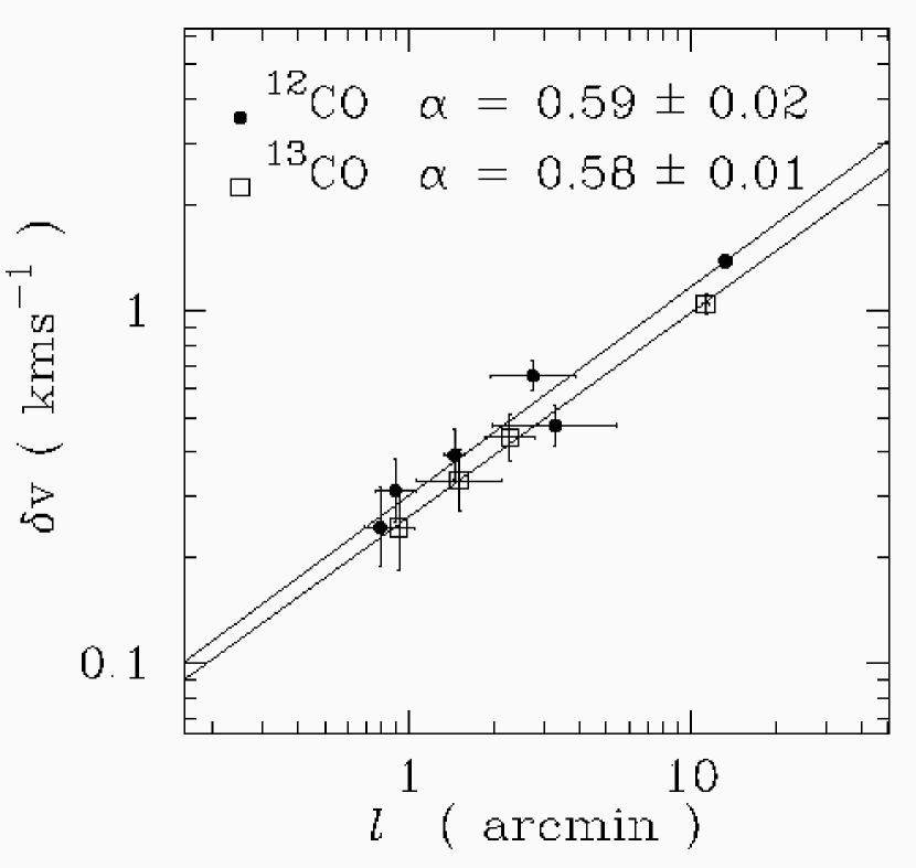
Figure 19: Principal component analysis results for the selected field. The solid lines are the fits to the ¹²CO (upper) and ¹³CO (lower) ${\delta}v$, $l$ pairs (${\delta}v$ $\propto$ $l^{\alpha}$).

The interpretation of existing results from line centroid analysis applied to molecular clouds in general will depend on the inferred, or assumed, state of turbulence. If molecular clouds are in an evolved state of decaying turbulence, then projection smoothing only applies, and we would infer $\gamma_{3D}$ $\approx$ 0 for all clouds studied to date. If, however, the clouds are still being strongly driven, or have only recently formed, then the $\delta\kappa$ $\approx$ –1 induced by density inhomogeneity should apply, and we thus can find a better consistency between line centroid analysis and other measures of $\gamma_{3D}$. To show this, we applied principal component analysis (PCA) to the analysis region according to the prescription given in Brunt & Heyer (2002) to derive a sequence of coupled characteristic scales, ${\delta}v$ and $\ell$, in velocity and space respectively. The results of this, yielding slightly better than an order of magnitude in spatial dynamic range, are shown in Figure 19. The ${\delta}v$ and $\ell$ pairs were fitted as ${\delta}v$ $\propto$ $\ell^{\alpha}$. We derive $\alpha$ $=$ 0.58 $\pm$ 0.01 (¹³CO) and $\alpha$ $=$ 0.59 $\pm$ 0.02 (¹²CO), resulting in $\gamma_{3D}$ $=$0.44 $\pm$ 0.01 (¹³CO) and $\gamma_{3D}$ $=$0.46 $\pm$ 0.04 (¹²CO) according to the Brunt (1999) calibration. Some caution is necessary here, though, on two counts. First, $\alpha$ is more directly dependent on the first order velocity fluctuation spectrum, not the second order spectrum that is traced by the power spectrum of the line centroid field; second, estimates of $\alpha$ are uncertain (around the mean calibration line) by $\sim$0.1 (Brunt et al. 2003). Neither of these factors can reconcile the PCA results with $\gamma_{3D}$ $\approx$ 0 however. If, as suggested by PCA in the limit of weak intermittency (as also supported by the lack of strong exponential tails in the line profiles), $\gamma_{3D}$ $\approx$ 0.45 then we infer that $\delta\kappa$ $\approx$ –0.9 would be needed to reconcile the line centroid results with PCA. This value of $\delta\kappa$ is consistent with $\delta\kappa$ $=$ –0.96 $\pm$ 0.22 derived from the numerical simulations of driven turbulence.

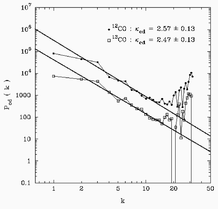
Figure 20: Output integrated intensity power spectra after noise floor subtraction and beam pattern division. The heavy lines are the fits of $\kappa_{cd}$ to these spectra in the range $k$ = 2 to $k$ = 13.

To determine the observationally-motivated value of $\delta\kappa$, without recourse to PCA, we examined the power spectra of the integrated intensity fields for both isotopes (it would be very difficult to attempt this with a hybrid integrated intensity field). Here, we assume that the integrated intensity field provides a good estimate of the column density field. To do this, we estimated the noise floor by integrating signal-free regions of the baseline over the same number of channels as was used to generate integrated intensity maps. The measured “column density” power spectra were then corrected for the noise floor and beam pattern (Equation 5) and the resulting output power spectra are shown in Figure 20. We have fitted $\kappa_{cd}$ over the range $k$ = 2 to $k$ = 13 (the same as used for the velocity line centroid power spectra), to estimate $\kappa_{cd}$ $\approx$ 2.5 consistently between the two isotopes. This is in general agreement with typical $\kappa_{cd}$ measured in molecular clouds (Bensch et al. 2001) but slightly smaller than can be accounted for by our numerical fields. Using Figure 9 as a rough guide, we interpret the measured $\kappa_{cd}$ as motivating $\delta\kappa$ $\approx$ –1. In doing this, we are considering the numerically simulated fields to be a more realistic representation of real molecular clouds than the phase-randomized versions. We do not see a turnover at small $k$ in the integrated intensity power spectra, nor in the velocity line centroid power spectra, except perhaps at $k$ = 1 which is quite uncertain. Our observed power spectra are thus more in accord with the numerical models driven at small wavenumber (see also Ossenkopf & Mac Low 2002). Finally, we used the ¹³CO data to provide an estimate of $\sigma_{N/N_{0}}$, by assuming that the ¹³CO is optically thin. To do this, we created an integrated intensity image of the emission and an integrated intensity image of instrumental noise over the same number of channels (64); the data were left in $T_{A}^{*}$ units, since the absolute scaling is unimportant. The mean integrated intensity of the data is : $I_{0}$ = 1.034 $\pm$0.004 K km s^-1. The total (signal+noise) standard deviation of the integrated intensity image is $\sigma_{I,tot}$ = 0.661. The contribution of the standard deviation of the noise is : $\sigma_{I,noise}~{}=~{}$ 0.253 K km s^-1. Thus we measure $\sigma_{I,signal/I_{0}}$ = 0.591 $\pm$0.004 which we take as being $\approx$ $\sigma_{N/N_{0}}$. This is clearly inconsistent with $\sigma_{N/N_{0}}$ = 0.065 seen in the phase-randomized density field (obtained with $\kappa_{cd}$ = 2.87) and referral to Figure 12(d) will show a good consistency between estimates of $\kappa_{cd}$ and $\sigma_{N/N_{0}}$ for the observational data compared to the numerical data. The effective spatial dynamic range in the simulations for computing $\sigma_{N/N_{0}}$ will lie between the nominal spatial dynamic range (128 per axis) and the most stringent interpretation of the maximum dissipation scale ($\sim$ 12.8 per axis). These compare reasonably well with the data, at a spatial dynamic range of 32 beams (64 pixels) per axis. We interpret the consistency found between $\kappa_{cd}$ and $\sigma_{N/N_{0}}$ as motivating the use of the numerically simulated fields to infer $\delta\kappa$ $\approx$ –1.

Our results regarding the effect of density inhomogeneity indicate that the measured $\kappa_{2D}$ $\sim$ 3 is thus shallower than the true $\kappa_{3D}$ by approximately $\delta\kappa$ $\approx$ –1, and we then infer $\kappa_{3D}$ $\approx$ 4 (c.f. Figure 8(c)) and thus $\gamma_{3D}$ $\approx$ 0.5. In more detail, we derive (using $\delta\kappa$ = –0.96 $\pm$ 0.22) $\kappa_{3D}$ = 4.07 $\pm$ 0.24 (¹²CO) and $\kappa_{3D}$ = 3.89 $\pm$ 0.26 (hybrid). These convert to : $\gamma_{3D}$ = 0.54 $\pm$ 0.12 (¹²CO) and $\gamma_{3D}$ = 0.45 $\pm$ 0.13 (hybrid). These are in good agreement with $\gamma_{3D}$ $\approx$ 0.45 determined from PCA, and are consistent with compressible, Burgers turbulence. The uncertainty in the inferred $\gamma_{3D}$ is large, due mainly to the intrinsic variability of $\delta\kappa$ ($\sim$ $\pm$ 0.22). We thus cannot entirely rule out the Kolmogorov case $\kappa_{3D}$ $\approx$ 3.67, $\gamma_{3D}$ $\approx$ 0.33, from velocity line centroid analysis alone, particularly if we include the extra uncertainties arising from subtraction of large scale gradients and edge effects (estimated to be $\sim$ $\pm$ 0.1 in $\kappa_{2D}$).

We interpret the conditions required for consistency between velocity line centroid analysis, principal component analysis and size-linewidth analysis as providing indirect support for molecular clouds that have only recently formed and/or are continually driven on large scales (Elmegreen 1993; Ballesteros-Paredes, Vázquez-Semadeni, & Scalo 1999).

Projection smoothing does not apply in the case that the line of sight depth over which the observational tracer exists is much less than the total transverse scale of emission observed on the sky, requiring sheet-like clouds, oriented face-on towards us. For a face-on sheet, the effect of density weighting would also vanish as there is no longer any line of sight variability (see Equation 3 in the limit that $N_{pix}$ $\longrightarrow$ 1 as a representation of this regime). While this solution is quite unsatisfactory in general, it represents a limiting case : no projection smoothing, no density weighting effects, resulting in the direct measurement of intrinsic statistical properties; i.e. the field is actually two dimensional. Some modified version of this limiting case may be operating in our numerical fields; i.e. in the case that a single density enhancement (not necessarily confined to a thin sheet, but having some spatial coherence) is dominant along the line of sight, then this will approximate the $N_{pix}$ $\longrightarrow$ 1 limit of Equation 3.

In general, for the full 3D (isotropic) driven case, our numerical results show that projection smoothing is countered by the effects of density inhomogeneity, again resulting in recovery of intrinsic statistical scaling properties, but in a less direct way.

7 Summary

We have examined numerical simulations of supersonic turbulence in molecular clouds in order to understand the effects of projection smoothing and density inhomogeneity on observable velocity line centroid fields ($v_{lc}(x,y)$). We find that the observed index, $\gamma_{2D}$, describing the variation of projected line centroid velocities ($\langle{\delta}v_{lc}^{2}\rangle^{1/2}$ $\propto$ $\ell^{\gamma_{2D}}$) is related to the intrinsic index, $\gamma_{3D}$, (where $\langle{\delta}v^{2}\rangle^{1/2}$ $\propto$ $\ell^{\gamma_{3D}}$) via the following relation :

$$\gamma_{2D}\;\;\;=\;\;\;\gamma_{3D}\;\;\;+\;\;\;0.5\;\;\;+\;\;\;\delta\kappa/2,$$

where the increase of 0.5 is a direct consequence of projection smoothing, and $\delta\kappa$ is an empirically determined correction for the effects of density inhomogeneity.

For driven turbulence, both with and without magnetic fields, $\delta\kappa$ $\approx$ –1 (with variations $\sim$ $\pm$ 0.22), thus implying $\gamma_{2D}$ $\approx$ $\gamma_{3D}$ due to the accidental cancellation of the effects of projection smoothing and small-scale structure induced by density inhomogeneity on the line centroid field. For decaying turbulence, $\delta\kappa$ tends to $\sim$0 at late times, so that $\gamma_{2D}$ $\approx$ $\gamma_{3D}$ + 0.5 due entirely to projection smoothing.

The variations in $\delta\kappa$ observed in high Mach number driven turbulence have no obvious dependence on Mach number, $M$. As $M\longrightarrow$0 (the incompressible case) one should also expect that $\delta\kappa\longrightarrow$0, as is indeed seen at late times in the decaying runs. We have inferred that $\delta\kappa$ is determined mostly by the amplitude of density fluctuations. The scatter in $\delta\kappa$ in the supersonic regime emphasizes the need for continued high spatial dynamic range surveying of the molecular ISM in order to provide a statistically useful sample of fields.

Deprojection of observed scaling relations in velocity line centroid fields requires some knowledge of the state of the flow. This information can be inferred from the spectral slope of the column density power spectrum and a measure of the standard deviation in column density relative to the mean ($\sigma_{N/N_{0}}$). Our numerical results show that $\gamma_{3D}$ is now consistently estimated at $\sim$0.5 using velocity line centroid analysis and using principal component analysis and size-linewidth relations. This consistency requires that molecular clouds are continually driven or only recently formed.

Table 1: Numerical Models : Parameters and Measurements

Model	$N_{pix}$	HD/MHD/Decay	$k_{d}$	M	$v_{A}/c_{s}$	t	$\delta\kappa$	$\kappa_{cd}$	$\sigma_{ln(\rho)}$	$\sigma_{ln(N)}$
HA8	128	HD	7–8	1.9	0	1	–0.84 $\pm$ 0.05	4.10 $\pm$ 0.12	0.71	0.17
HC2	128	HD	1–2	7.4	0	1	–0.72 $\pm$ 0.05	3.30 $\pm$ 0.13	1.58	0.71
HC4	128	HD	3–4	5.3	0	1	–0.98 $\pm$ 0.03	3.22 $\pm$ 0.09	1.55	0.48
HC8	128	HD	7–8	4.1	0	1	–1.17 $\pm$ 0.06	3.36 $\pm$ 0.08	1.34	0.32
HE2	128	HD	1–2	15.0	0	0.475	–1.04 $\pm$ 0.05	2.87 $\pm$ 0.10	2.45	0.74
HE4	128	HD	3–4	12.0	0	0.875	–1.11 $\pm$ 0.06	3.02 $\pm$ 0.09	2.23	0.63
HE8	128	HD	7–8	8.7	0	1	–1.28 $\pm$ 0.11	3.14 $\pm$ 0.09	2.07	0.40
MC4X $v_{\perp}$	128	MHD	3–4	5.3	10	0.1	–0.91 $\pm$ 0.12	3.04 $\pm$ 0.09	1.68	0.56
MC4X $v_{||}$	128	MHD	3–4	5.3	10	0.1	–1.21 $\pm$ 0.05	2.57 $\pm$ 0.09	1.68	0.46
MC45 $v_{\perp}$	128	MHD	3–4	4.8	5	0.2	–0.66 $\pm$ 0.09	3.03 $\pm$ 0.13	1.58	0.45
MC45 $v_{||}$	128	MHD	3–4	4.8	5	0.2	–1.06 $\pm$ 0.05	2.93 $\pm$ 0.11	1.58	0.48
MC41 $v_{\perp}$	128	MHD	3–4	4.7	1	0.5	–0.89 $\pm$ 0.05	3.18 $\pm$ 0.08	1.28	0.36
MC41 $v_{||}$	128	MHD	3–4	4.7	1	0.5	–0.71 $\pm$ 0.05	3.20 $\pm$ 0.09	1.28	0.32
MC85 $v_{\perp}$	128	MHD	7–8	3.4	5	0.075	–0.59 $\pm$ 0.11	3.31 $\pm$ 0.10	1.50	0.32
MC85 $v_{||}$	128	MHD	7–8	3.4	5	0.075	–1.31 $\pm$ 0.08	2.93 $\pm$ 0.09	1.50	0.30
MC81 $v_{\perp}$	128	MHD	7–8	3.5	1	0.225	–1.00 $\pm$ 0.07	3.41 $\pm$ 0.09	1.18	0.27
MC81 $v_{||}$	128	MHD	7–8	3.5	1	0.225	–1.09 $\pm$ 0.06	3.38 $\pm$ 0.08	1.18	0.28
ME21 $v_{\perp}$	128	MHD	1–2	14.0	1	0.5	–0.85 $\pm$ 0.06	3.22 $\pm$ 0.09	1.90	0.77
ME21 $v_{||}$	128	MHD	1–2	14.0	1	0.5	–0.81 $\pm$ 0.07	3.15 $\pm$ 0.08	1.90	1.27
D	256	HD/Decay	1–8	5.0	0	0.1	–0.76 $\pm$ 0.03	4.39 $\pm$ 0.08	0.68	0.19
D	256	HD/Decay	1–8	5.0	0	0.15	–0.59 $\pm$ 0.02	4.70 $\pm$ 0.08	0.54	0.17
D	256	HD/Decay	1–8	5.0	0	0.3	–0.32 $\pm$ 0.02	5.13 $\pm$ 0.09	0.37	0.13
D	256	HD/Decay	1–8	5.0	0	0.5	–0.14 $\pm$ 0.01	5.44 $\pm$ 0.09	0.26	0.09
U	256	HD/Decay	1–8	50.0	0	0.1	–0.97 $\pm$ 0.03	4.09 $\pm$ 0.07	0.97	0.35
U	256	HD/Decay	1–8	50.0	0	0.15	–0.86 $\pm$ 0.02	4.48 $\pm$ 0.09	0.81	0.30
U	256	HD/Decay	1–8	50.0	0	0.3	–0.48 $\pm$ 0.02	4.93 $\pm$ 0.07	0.51	0.21
U	256	HD/Decay	1–8	50.0	0	0.5	–0.29 $\pm$ 0.01	5.17 $\pm$ 0.08	0.40	0.15

Figure 4: Variation of $P_{v_{lc}^{wgt}}$$/$$P_{v_{lc}^{true}}$ with $k$ for the decaying turbulence simulations as time progresses. Fits (heavy lines) to derive $\delta\kappa$ were made in the range of $k$ delimited by the dashed lines ($k$ = 10 to $k$ = 64). Each plot is labeled by the time step in units of the sound crossing time. (Left: model D, initial $M$ = 5. Right: model U, initial $M$ = 50.)

Figure 14: Example fitted Gaussians (heavy lines) to the observed spectra (lighter lines) in the analysis region.

Figure 17: Overview of the relevant terms necessary to construct the output line centroid power spectra. (a) ¹²CO field; raw observed power spectrum, noise floor and beam pattern (45″); (b) same for the hybrid field; the dashed line is the 46″ beam pattern applicable to the ¹³CO data; no uncertainty arises from applying the 45″ beam pattern to the hybrid field.

References

- Ballesteros-Paredes et al. (1999) Ballesteros-Paredes, J., Vázquez-Semadeni, E., & Scalo, J. 1999, ApJ, 515, 286
- Ballesteros-Paredes & Mac Low (2002) Ballesteros-Paredes, J., & Mac Low, M.-M., 2002, ApJ, 570, 734
- Bensch et al. (2001) Bensch, F., Stutzki, J., & Ossenkopf, V., 2001, A&A, 366, 636
- Brunt (1999) Brunt, C.M., 1999, Ph.D. Thesis, Univ. Massachusetts at Amherst
- Brunt & Heyer (2002) Brunt, C.M., & Heyer, M.H., 2002, ApJ, 556, 276 (Paper I)
- Brunt et al. (2003) Brunt, C.M., Heyer, M.H., Vázquez-Semadeni, E., & Pichardo, B., 2003, ApJ, in press, ApJ Preprint doi:10.1086/377479
- Burgers (1974) Burgers, J.M., 1974, The Nonlinear Diffusion Equation (Dordrecht: Reidel)
- Cho & Lazarian (2002) Cho, J., & Lazarian, A., 2002, Phys. Rev. Lett., 88, 245001
- Clarke (1994) Clarke, D., 1994, NCSA Technical Report
- Dickman & Kleiner (1985) Dickman, R.L., & Kleiner, S.C., 1985, ApJ, 295, 479
- Elmegreen (1993) Elmegreen, B.G., 1993, ApJ, 419, L29
- Erickson et al. (1999) Erickson, N. R., Grosslein, R. M., Erickson, R. B., & Weinreb, S. 1999, IEEE Trans. Microwave Theory Tech., 47, 2212
- Evans & Hawley (1988) Evans, C.R., & Hawley, J.F., 1988, ApJ, 332, 659
- (14) Falgarone, É. Lis, D.C., Phillips, T.G., Pouquet, A., Porter, A. & Woodward, P.R., 1994, ApJ, 436, 728
- Hawley & Stone (1995) Hawley, J.F., & Stone, J.M., 1995, Comp. Phys. Comm., 89, 127
- Heyer & Schloerb (1997) Heyer, M.H. & Schloerb, F.P., 1997, ApJ, 475, 173
- Hobson (1992) Hobson, M.P., 1992, MNRAS, 256, 457
- von Hoerner (1951) von Hoerner, S., 1951, Zeitschrift für Astrophysik, 30, 17
- Kitamura et al. (1993) Kitamura, Y., Sunada, K., Hayashi, M., & Hasegawa, T., 1993, ApJ, 413, 221
- Kleiner & Dickman (1985) Kleiner, S.C. & Dickman, R.L. 1985, ApJ, 295, 466
- Kolmogorov (1941) Kolmogorov, A.N., 1941, Dokl. Akad. Nauk SSR, 30, 301
- Kutner & Ulich (1981) Kutner, M.L., & Ulich, B.L., 1981, ApJ, 250, 341