The Response of a Two-Element Radio Interferometer to Gravitational Waves

Abstract

This document presents a ray-optics analysis of the response of a two-element radio interferometer to the presence of a plane gravitational wave. A general expression for the differential phase observed between the two receiving stations as a result of an arbitrary gravitational wave is determined, as well as the specific responses to monochromatic and black hole ring-down waveforms. Finally, the possibility of gravitational wave detection via this mechanism is discussed in the context of interferometer noise.

I Introduction

A gravitational wave is a perturbation to the geometry of space that propagates through space at the speed of light. It’s effect is to stretch and shrink the distances between objects in the directions transverse to its direction of travel. The distortion is volume-preserving, so while it is shrinking distances in one direction, it stretches them in another.

The stretching and shrinking effect is not a co-ordinate artifact. A measuring stick used to monitor the distance between two objects freely-falling in the presence of a gravitational wave will measure one separation distance at one time and a different separation later. The stretching and shrinking is also linear: given the change in distance between two objects separated by a distance $L$, the change in distance between two objects separated by $2L$ will be doubled. The amplitude of a gravitational wave is expressed as a dimensionless quantity giving the change in distance per unit distance — a shear strain in space.

Any apparatus capable of accurately measuring the distance between two objects, or the change in the distance between two objects, as a function of time is, in principle, capable of detecting a gravitational wave. The question of the effectiveness of the apparatus in accomplishing this task is one of sensitivity and signal-to-noise ratio. One design being actively pursued by several research groups today is based on a Michelson-type laser interferometer. In this design, a laser beam is split and sent down the two orthogonal arms of the apparatus, and then at the end of each is reflected off a suspended mass back toward the splitter where the beams are recombined Abramovici et al. (1992); Caron et al. (1997); Danzmann (1997); Lück and the GEO600 Team (1997); Kawabe and the TAMA collaboration (1997). If the length of one or the other arms changes, the result will be a change in the differential phase between the returning laser beams and so a passing gravitational wave will appear as a shift in the interference pattern at the output of the interferometer. A variation on this technique that is also being pursued by several research groups is a detector consisting of an Earth-based transmitter/receiver and a spacecraft carrying a radio or optical transponder. There are currently proposals to launch specially-designed vehicles dedicated to this task using optical links from the ground to the vehicle and back Ni (2002). It is also possible to use existing missions. Deep-space vehicles generally carry radio transponders that are used as aids to navigation. By maintaining a coherent up-link/down-link channel at high frequency stability with appropriate modulations one can measure the range and range-rate to the spacecraft with high precision and thereby search for the passage of a gravitational wave through the solar system Bertotti et al. (1998).

In this document, another type of gravitational wave detection apparatus similar to this last technique is introduced and investigated. Figure 1 shows a radio interferometer arrangement with a distant radio source and two receiving elements.

Figure 1: A gravitational wave moving across the lines of sight in the plane of a two-station interferometer. One of the gravitational wave’s polarization axes is aligned (ignoring parallax) with the lines of sight.

It also shows a gravitational wave travelling across the lines of sight to the radio source in the plane defined by the source and the two interferometer elements (to be referred to, hereinafter, as the plane of the interferometer). For the purpose of illustration, one of the gravitational wave’s polarization axes is aligned (ignoring parallax) with the lines of sight. Because the gravitational wave travels at finite speed, any perturbation to distances transverse to its direction of travel will influence the signal arriving at receiver 1 in advance of its influence on the signal arriving at receiver 2. The presence of a gravitational wave will, therefore, manifest itself as a time-varying difference between the arrival times of radio signals at the receivers — a time-varying differential phase between the stations. Such a detector is similar in operation to the single arm, spacecraft-based, coherent up-link/down-link type of detector. In this case, however, a second arm is introduced to act as a phase reference for the first which permits the use of a broad-band radio signal. What follows is an analysis of the magnitude of the differential phase between the stations when a gravitational wave is present, and a preliminary assessment of the signal-to-noise ratio in this type of detector.

We will consider a radio signal emanating from the radio source toward each of the receiving stations. Each radio signal is treated as a null geodesic in space-time, originating on the radio source’s world line. The intersections of the geodesics with the world lines of the receivers define events in space-time giving the co-ordinate times of arrival of the signal at each receiving element. By determining the difference in the times of emission of the signals being received simultaneously at the two receiving elements, and multiplying this time difference by the angular frequency of the radio emission one obtains the differential phase between the two receiving elements. The calculation will first be done for arbitrary receiver locations and arbitrary gravitational waveforms, then a simplified interferometer arrangement will be introduced in order to more easily discuss the response to specific gravitational waves. Throughout the calculations, the units for length will be chosen so as to make the numerical value of the speed of light, $c$, equal to 1.

II Null Geodesics in a Plane Gravitational Wave Space-Time

For simplicity, we assume a Minkowski background for the geometry of space-time. Rather than solving the geodesic equation for fixed radio source and receiver positions in an arbitrarily-oriented gravitational wave, we shall choose to fix the orientation of the gravitational wave and adjust the geodesic’s end-points. The co-ordinate system is defined as follows: the radio source locates the origin of the spatial co-ordinates, the gravitational wave vector sets the negative-$z$ direction and the two polarization axes of the gravitational wave set the $x$ and $y$ directions. The origin of the time co-ordinate is arbitrary. Space-time geometry is described by the metric tensor

$$\mathchoice{g_{\kern 0.0pt\hbox{$\scriptstyle\mu\nu$}}}{g_{\kern 0.0pt\hbox{$\scriptstyle\mu\nu$}}}{g_{\kern 0.0pt\hbox{$\scriptscriptstyle\mu\nu$}}}{g_{\kern 0.0pt\hbox{$\scriptscriptstyle\mu\nu$}}}=\mathchoice{\eta_{\kern 0.0pt\hbox{$\scriptstyle\mu\nu$}}}{\eta_{\kern 0.0pt\hbox{$\scriptstyle\mu\nu$}}}{\eta_{\kern 0.0pt\hbox{$\scriptscriptstyle\mu\nu$}}}{\eta_{\kern 0.0pt\hbox{$\scriptscriptstyle\mu\nu$}}}+\mathchoice{h_{\kern 0.0pt\hbox{$\scriptstyle\mu\nu$}}}{h_{\kern 0.0pt\hbox{$\scriptstyle\mu\nu$}}}{h_{\kern 0.0pt\hbox{$\scriptscriptstyle\mu\nu$}}}{h_{\kern 0.0pt\hbox{$\scriptscriptstyle\mu\nu$}}},$$ (1)

where the background Minkowski metric tensor is

$$\mathchoice{\eta_{\kern 0.0pt\hbox{$\scriptstyle\mu\nu$}}}{\eta_{\kern 0.0pt\hbox{$\scriptstyle\mu\nu$}}}{\eta_{\kern 0.0pt\hbox{$\scriptscriptstyle\mu\nu$}}}{\eta_{\kern 0.0pt\hbox{$\scriptscriptstyle\mu\nu$}}}=\operatorname{diag}(-1,1,1,1),$$ (2)

and the gravitational wave is described by the tensor $\mathchoice{h_{\kern 0.0pt\hbox{$\scriptstyle\mu\nu$}}}{h_{\kern 0.0pt\hbox{$\scriptstyle\mu\nu$}}}{h_{\kern 0.0pt\hbox{$\scriptscriptstyle\mu\nu$}}}{h_{\kern 0.0pt\hbox{$\scriptscriptstyle\mu\nu$}}}$ given by

$$\mathchoice{h_{\kern 0.0pt\hbox{$\scriptstyle\mu\nu$}}}{h_{\kern 0.0pt\hbox{$\scriptstyle\mu\nu$}}}{h_{\kern 0.0pt\hbox{$\scriptscriptstyle\mu\nu$}}}{h_{\kern 0.0pt\hbox{$\scriptscriptstyle\mu\nu$}}}=h(z+t)\mathchoice{e^{+}_{\kern 0.0pt\hbox{$\scriptstyle\mu\nu$}}}{e^{+}_{\kern 0.0pt\hbox{$\scriptstyle\mu\nu$}}}{e^{+}_{\kern 0.0pt\hbox{$\scriptscriptstyle\mu\nu$}}}{e^{+}_{\kern 0.0pt\hbox{$\scriptscriptstyle\mu\nu$}}}.$$ (3)

$\mathchoice{e^{+}_{\kern 0.0pt\hbox{$\scriptstyle\mu\nu$}}}{e^{+}_{\kern 0.0pt\hbox{$\scriptstyle\mu\nu$}}}{e^{+}_{\kern 0.0pt\hbox{$\scriptscriptstyle\mu\nu$}}}{e^{+}_{\kern 0.0pt\hbox{$\scriptscriptstyle\mu\nu$}}}$ is the gravitational wave’s polarization tensor which, in this case, is

$$\mathchoice{e^{+}_{\kern 0.0pt\hbox{$\scriptstyle\mu\nu$}}}{e^{+}_{\kern 0.0pt\hbox{$\scriptstyle\mu\nu$}}}{e^{+}_{\kern 0.0pt\hbox{$\scriptscriptstyle\mu\nu$}}}{e^{+}_{\kern 0.0pt\hbox{$\scriptscriptstyle\mu\nu$}}}=\operatorname{diag}(0,1,-1,0),$$ (4)

and $h(z+t)$ is the gravitational wave’s amplitude and describes a waveform propagating at the speed of light in the negative $z$ direction. $h(z+t)$ carries units of strain — change in length per unit length — making it dimensionless. Since the radio source defines the origin of the spatial co-ordinates, the calculations are being done in its rest frame so co-ordinate time corresponds to the proper time measured by a clock carried by the radio source. This may or may not agree with the proper times measured at the receiving elements.

We assume the amplitude of the gravitational wave is small, $\left|h\right|\ll 1$, and carry out calculations to first order in $h$. Altogether, the line element describing the geometry of space-time is

$$\,\mathrm{d}s^{2}=-\,\mathrm{d}t^{2}+\left[1+h(z+t)\right]\,\mathrm{d}x^{2}+\\ \left[1-h(z+t)\right]\,\mathrm{d}y^{2}+\,\mathrm{d}z^{2}.$$ (5)

The only non-zero Christoffel symbols for this line element are

$$\mathchoice{\Gamma_{\kern 0.0pt\hbox{$\scriptstyle\hbox{}xx$}}^{\hbox{$\scriptstyle{}$}\kern 0.0pt\hbox{$\kern 0.0pt\scriptstyle t\hbox{}\hbox{}$}}}{\Gamma_{\kern 0.0pt\hbox{$\scriptstyle\hbox{}xx$}}^{\hbox{$\scriptstyle{}$}\kern 0.0pt\hbox{$\kern 0.0pt\scriptstyle t\hbox{}\hbox{}$}}}{\Gamma_{\kern 0.0pt\hbox{$\scriptscriptstyle\hbox{}xx$}}^{\hbox{$\scriptscriptstyle{}$}\kern 0.0pt\hbox{$\kern 0.0pt\scriptscriptstyle t\hbox{}\hbox{}$}}}{\Gamma_{\kern 0.0pt\hbox{$\scriptscriptstyle\hbox{}xx$}}^{\hbox{$\scriptscriptstyle{}$}\kern 0.0pt\hbox{$\kern 0.0pt\scriptscriptstyle t\hbox{}\hbox{}$}}}=-\mathchoice{\Gamma_{\kern 0.0pt\hbox{$\scriptstyle\hbox{}yy$}}^{\hbox{$\scriptstyle{}$}\kern 0.0pt\hbox{$\kern 0.0pt\scriptstyle t\hbox{}\hbox{}$}}}{\Gamma_{\kern 0.0pt\hbox{$\scriptstyle\hbox{}yy$}}^{\hbox{$\scriptstyle{}$}\kern 0.0pt\hbox{$\kern 0.0pt\scriptstyle t\hbox{}\hbox{}$}}}{\Gamma_{\kern 0.0pt\hbox{$\scriptscriptstyle\hbox{}yy$}}^{\hbox{$\scriptscriptstyle{}$}\kern 0.0pt\hbox{$\kern 0.0pt\scriptscriptstyle t\hbox{}\hbox{}$}}}{\Gamma_{\kern 0.0pt\hbox{$\scriptscriptstyle\hbox{}yy$}}^{\hbox{$\scriptscriptstyle{}$}\kern 0.0pt\hbox{$\kern 0.0pt\scriptscriptstyle t\hbox{}\hbox{}$}}}=\frac{1}{2}h^{\prime}(z+t)$$

$$\mathchoice{\Gamma_{\kern 0.0pt\hbox{$\scriptstyle\hbox{}xx$}}^{\hbox{$\scriptstyle{}$}\kern 0.0pt\hbox{$\kern 0.0pt\scriptstyle z\hbox{}\hbox{}$}}}{\Gamma_{\kern 0.0pt\hbox{$\scriptstyle\hbox{}xx$}}^{\hbox{$\scriptstyle{}$}\kern 0.0pt\hbox{$\kern 0.0pt\scriptstyle z\hbox{}\hbox{}$}}}{\Gamma_{\kern 0.0pt\hbox{$\scriptscriptstyle\hbox{}xx$}}^{\hbox{$\scriptscriptstyle{}$}\kern 0.0pt\hbox{$\kern 0.0pt\scriptscriptstyle z\hbox{}\hbox{}$}}}{\Gamma_{\kern 0.0pt\hbox{$\scriptscriptstyle\hbox{}xx$}}^{\hbox{$\scriptscriptstyle{}$}\kern 0.0pt\hbox{$\kern 0.0pt\scriptscriptstyle z\hbox{}\hbox{}$}}}=-\mathchoice{\Gamma_{\kern 0.0pt\hbox{$\scriptstyle\hbox{}yy$}}^{\hbox{$\scriptstyle{}$}\kern 0.0pt\hbox{$\kern 0.0pt\scriptstyle z\hbox{}\hbox{}$}}}{\Gamma_{\kern 0.0pt\hbox{$\scriptstyle\hbox{}yy$}}^{\hbox{$\scriptstyle{}$}\kern 0.0pt\hbox{$\kern 0.0pt\scriptstyle z\hbox{}\hbox{}$}}}{\Gamma_{\kern 0.0pt\hbox{$\scriptscriptstyle\hbox{}yy$}}^{\hbox{$\scriptscriptstyle{}$}\kern 0.0pt\hbox{$\kern 0.0pt\scriptscriptstyle z\hbox{}\hbox{}$}}}{\Gamma_{\kern 0.0pt\hbox{$\scriptscriptstyle\hbox{}yy$}}^{\hbox{$\scriptscriptstyle{}$}\kern 0.0pt\hbox{$\kern 0.0pt\scriptscriptstyle z\hbox{}\hbox{}$}}}=-\frac{1}{2}h^{\prime}(z+t)$$

$$\mathchoice{\Gamma_{\kern 0.0pt\hbox{$\scriptstyle\hbox{}tx$}}^{\hbox{$\scriptstyle{}$}\kern 0.0pt\hbox{$\kern 0.0pt\scriptstyle x\hbox{}\hbox{}$}}}{\Gamma_{\kern 0.0pt\hbox{$\scriptstyle\hbox{}tx$}}^{\hbox{$\scriptstyle{}$}\kern 0.0pt\hbox{$\kern 0.0pt\scriptstyle x\hbox{}\hbox{}$}}}{\Gamma_{\kern 0.0pt\hbox{$\scriptscriptstyle\hbox{}tx$}}^{\hbox{$\scriptscriptstyle{}$}\kern 0.0pt\hbox{$\kern 0.0pt\scriptscriptstyle x\hbox{}\hbox{}$}}}{\Gamma_{\kern 0.0pt\hbox{$\scriptscriptstyle\hbox{}tx$}}^{\hbox{$\scriptscriptstyle{}$}\kern 0.0pt\hbox{$\kern 0.0pt\scriptscriptstyle x\hbox{}\hbox{}$}}}=\mathchoice{\Gamma_{\kern 0.0pt\hbox{$\scriptstyle\hbox{}xt$}}^{\hbox{$\scriptstyle{}$}\kern 0.0pt\hbox{$\kern 0.0pt\scriptstyle x\hbox{}\hbox{}$}}}{\Gamma_{\kern 0.0pt\hbox{$\scriptstyle\hbox{}xt$}}^{\hbox{$\scriptstyle{}$}\kern 0.0pt\hbox{$\kern 0.0pt\scriptstyle x\hbox{}\hbox{}$}}}{\Gamma_{\kern 0.0pt\hbox{$\scriptscriptstyle\hbox{}xt$}}^{\hbox{$\scriptscriptstyle{}$}\kern 0.0pt\hbox{$\kern 0.0pt\scriptscriptstyle x\hbox{}\hbox{}$}}}{\Gamma_{\kern 0.0pt\hbox{$\scriptscriptstyle\hbox{}xt$}}^{\hbox{$\scriptscriptstyle{}$}\kern 0.0pt\hbox{$\kern 0.0pt\scriptscriptstyle x\hbox{}\hbox{}$}}}=\frac{1}{2}h^{\prime}(z+t)$$

$$\mathchoice{\Gamma_{\kern 0.0pt\hbox{$\scriptstyle\hbox{}zx$}}^{\hbox{$\scriptstyle{}$}\kern 0.0pt\hbox{$\kern 0.0pt\scriptstyle x\hbox{}\hbox{}$}}}{\Gamma_{\kern 0.0pt\hbox{$\scriptstyle\hbox{}zx$}}^{\hbox{$\scriptstyle{}$}\kern 0.0pt\hbox{$\kern 0.0pt\scriptstyle x\hbox{}\hbox{}$}}}{\Gamma_{\kern 0.0pt\hbox{$\scriptscriptstyle\hbox{}zx$}}^{\hbox{$\scriptscriptstyle{}$}\kern 0.0pt\hbox{$\kern 0.0pt\scriptscriptstyle x\hbox{}\hbox{}$}}}{\Gamma_{\kern 0.0pt\hbox{$\scriptscriptstyle\hbox{}zx$}}^{\hbox{$\scriptscriptstyle{}$}\kern 0.0pt\hbox{$\kern 0.0pt\scriptscriptstyle x\hbox{}\hbox{}$}}}=\mathchoice{\Gamma_{\kern 0.0pt\hbox{$\scriptstyle\hbox{}xz$}}^{\hbox{$\scriptstyle{}$}\kern 0.0pt\hbox{$\kern 0.0pt\scriptstyle x\hbox{}\hbox{}$}}}{\Gamma_{\kern 0.0pt\hbox{$\scriptstyle\hbox{}xz$}}^{\hbox{$\scriptstyle{}$}\kern 0.0pt\hbox{$\kern 0.0pt\scriptstyle x\hbox{}\hbox{}$}}}{\Gamma_{\kern 0.0pt\hbox{$\scriptscriptstyle\hbox{}xz$}}^{\hbox{$\scriptscriptstyle{}$}\kern 0.0pt\hbox{$\kern 0.0pt\scriptscriptstyle x\hbox{}\hbox{}$}}}{\Gamma_{\kern 0.0pt\hbox{$\scriptscriptstyle\hbox{}xz$}}^{\hbox{$\scriptscriptstyle{}$}\kern 0.0pt\hbox{$\kern 0.0pt\scriptscriptstyle x\hbox{}\hbox{}$}}}=\frac{1}{2}h^{\prime}(z+t)$$

$$\mathchoice{\Gamma_{\kern 0.0pt\hbox{$\scriptstyle\hbox{}ty$}}^{\hbox{$\scriptstyle{}$}\kern 0.0pt\hbox{$\kern 0.0pt\scriptstyle y\hbox{}\hbox{}$}}}{\Gamma_{\kern 0.0pt\hbox{$\scriptstyle\hbox{}ty$}}^{\hbox{$\scriptstyle{}$}\kern 0.0pt\hbox{$\kern 0.0pt\scriptstyle y\hbox{}\hbox{}$}}}{\Gamma_{\kern 0.0pt\hbox{$\scriptscriptstyle\hbox{}ty$}}^{\hbox{$\scriptscriptstyle{}$}\kern 0.0pt\hbox{$\kern 0.0pt\scriptscriptstyle y\hbox{}\hbox{}$}}}{\Gamma_{\kern 0.0pt\hbox{$\scriptscriptstyle\hbox{}ty$}}^{\hbox{$\scriptscriptstyle{}$}\kern 0.0pt\hbox{$\kern 0.0pt\scriptscriptstyle y\hbox{}\hbox{}$}}}=\mathchoice{\Gamma_{\kern 0.0pt\hbox{$\scriptstyle\hbox{}yt$}}^{\hbox{$\scriptstyle{}$}\kern 0.0pt\hbox{$\kern 0.0pt\scriptstyle y\hbox{}\hbox{}$}}}{\Gamma_{\kern 0.0pt\hbox{$\scriptstyle\hbox{}yt$}}^{\hbox{$\scriptstyle{}$}\kern 0.0pt\hbox{$\kern 0.0pt\scriptstyle y\hbox{}\hbox{}$}}}{\Gamma_{\kern 0.0pt\hbox{$\scriptscriptstyle\hbox{}yt$}}^{\hbox{$\scriptscriptstyle{}$}\kern 0.0pt\hbox{$\kern 0.0pt\scriptscriptstyle y\hbox{}\hbox{}$}}}{\Gamma_{\kern 0.0pt\hbox{$\scriptscriptstyle\hbox{}yt$}}^{\hbox{$\scriptscriptstyle{}$}\kern 0.0pt\hbox{$\kern 0.0pt\scriptscriptstyle y\hbox{}\hbox{}$}}}=-\frac{1}{2}h^{\prime}(z+t)$$

$$\mathchoice{\Gamma_{\kern 0.0pt\hbox{$\scriptstyle\hbox{}zy$}}^{\hbox{$\scriptstyle{}$}\kern 0.0pt\hbox{$\kern 0.0pt\scriptstyle y\hbox{}\hbox{}$}}}{\Gamma_{\kern 0.0pt\hbox{$\scriptstyle\hbox{}zy$}}^{\hbox{$\scriptstyle{}$}\kern 0.0pt\hbox{$\kern 0.0pt\scriptstyle y\hbox{}\hbox{}$}}}{\Gamma_{\kern 0.0pt\hbox{$\scriptscriptstyle\hbox{}zy$}}^{\hbox{$\scriptscriptstyle{}$}\kern 0.0pt\hbox{$\kern 0.0pt\scriptscriptstyle y\hbox{}\hbox{}$}}}{\Gamma_{\kern 0.0pt\hbox{$\scriptscriptstyle\hbox{}zy$}}^{\hbox{$\scriptscriptstyle{}$}\kern 0.0pt\hbox{$\kern 0.0pt\scriptscriptstyle y\hbox{}\hbox{}$}}}=\mathchoice{\Gamma_{\kern 0.0pt\hbox{$\scriptstyle\hbox{}yz$}}^{\hbox{$\scriptstyle{}$}\kern 0.0pt\hbox{$\kern 0.0pt\scriptstyle y\hbox{}\hbox{}$}}}{\Gamma_{\kern 0.0pt\hbox{$\scriptstyle\hbox{}yz$}}^{\hbox{$\scriptstyle{}$}\kern 0.0pt\hbox{$\kern 0.0pt\scriptstyle y\hbox{}\hbox{}$}}}{\Gamma_{\kern 0.0pt\hbox{$\scriptscriptstyle\hbox{}yz$}}^{\hbox{$\scriptscriptstyle{}$}\kern 0.0pt\hbox{$\kern 0.0pt\scriptscriptstyle y\hbox{}\hbox{}$}}}{\Gamma_{\kern 0.0pt\hbox{$\scriptscriptstyle\hbox{}yz$}}^{\hbox{$\scriptscriptstyle{}$}\kern 0.0pt\hbox{$\kern 0.0pt\scriptscriptstyle y\hbox{}\hbox{}$}}}=-\frac{1}{2}h^{\prime}(z+t),$$

where $h^{\prime}$ is the derivative of $h$ with respect to its argument: $h^{\prime}(z+t)=\frac{\,\mathrm{d}}{\,\mathrm{d}(z+t)}h(z+t)$. A geodesic in the space-time is a solution of the geodesic equation,

$$\frac{\,\mathrm{d}^{2}\mathchoice{x^{\hbox{$\scriptstyle{}$}\kern 0.0pt\hbox{$\kern 0.0pt\scriptstyle\mu$}}}{x^{\hbox{$\scriptstyle{}$}\kern 0.0pt\hbox{$\kern 0.0pt\scriptstyle\mu$}}}{x^{\hbox{$\scriptscriptstyle{}$}\kern 0.0pt\hbox{$\kern 0.0pt\scriptscriptstyle\mu$}}}{x^{\hbox{$\scriptscriptstyle{}$}\kern 0.0pt\hbox{$\kern 0.0pt\scriptscriptstyle\mu$}}}}{\,\mathrm{d}\lambda^{2}}+\mathchoice{\Gamma_{\kern 0.0pt\hbox{$\scriptstyle\hbox{}\alpha\beta$}}^{\hbox{$\scriptstyle{}$}\kern 0.0pt\hbox{$\kern 0.0pt\scriptstyle\mu\hbox{}\hbox{}$}}}{\Gamma_{\kern 0.0pt\hbox{$\scriptstyle\hbox{}\alpha\beta$}}^{\hbox{$\scriptstyle{}$}\kern 0.0pt\hbox{$\kern 0.0pt\scriptstyle\mu\hbox{}\hbox{}$}}}{\Gamma_{\kern 0.0pt\hbox{$\scriptscriptstyle\hbox{}\alpha\beta$}}^{\hbox{$\scriptscriptstyle{}$}\kern 0.0pt\hbox{$\kern 0.0pt\scriptscriptstyle\mu\hbox{}\hbox{}$}}}{\Gamma_{\kern 0.0pt\hbox{$\scriptscriptstyle\hbox{}\alpha\beta$}}^{\hbox{$\scriptscriptstyle{}$}\kern 0.0pt\hbox{$\kern 0.0pt\scriptscriptstyle\mu\hbox{}\hbox{}$}}}\frac{\,\mathrm{d}\mathchoice{x^{\hbox{$\scriptstyle{}$}\kern 0.0pt\hbox{$\kern 0.0pt\scriptstyle\alpha$}}}{x^{\hbox{$\scriptstyle{}$}\kern 0.0pt\hbox{$\kern 0.0pt\scriptstyle\alpha$}}}{x^{\hbox{$\scriptscriptstyle{}$}\kern 0.0pt\hbox{$\kern 0.0pt\scriptscriptstyle\alpha$}}}{x^{\hbox{$\scriptscriptstyle{}$}\kern 0.0pt\hbox{$\kern 0.0pt\scriptscriptstyle\alpha$}}}}{\,\mathrm{d}\lambda}\frac{\,\mathrm{d}\mathchoice{x^{\hbox{$\scriptstyle{}$}\kern 0.0pt\hbox{$\kern 0.0pt\scriptstyle\beta$}}}{x^{\hbox{$\scriptstyle{}$}\kern 0.0pt\hbox{$\kern 0.0pt\scriptstyle\beta$}}}{x^{\hbox{$\scriptscriptstyle{}$}\kern 0.0pt\hbox{$\kern 0.0pt\scriptscriptstyle\beta$}}}{x^{\hbox{$\scriptscriptstyle{}$}\kern 0.0pt\hbox{$\kern 0.0pt\scriptscriptstyle\beta$}}}}{\,\mathrm{d}\lambda}=0,$$ (6)

and is described by four functions of an affine parameter: $x(\lambda)$, $y(\lambda)$, $z(\lambda)$, and $t(\lambda)$, where $\lambda$ parameterizes events along the the geodesic. Using the Christoffel symbols from above in the geodesic equation leads to the following four coupled, second-order, non-linear, differential equations for $x(\lambda)$, $y(\lambda)$, $z(\lambda)$, and $t(\lambda)$ along a geodesic in this space-time:

$$\frac{\,\mathrm{d}^{2}t}{\,\mathrm{d}\lambda^{2}}+\frac{1}{2}h^{\prime}(z+t)\left[\left(\frac{\,\mathrm{d}x}{\,\mathrm{d}\lambda}\right)^{2}-\left(\frac{\,\mathrm{d}y}{\,\mathrm{d}\lambda}\right)^{2}\right]=0,$$ (7a)

$$\frac{\,\mathrm{d}^{2}x}{\,\mathrm{d}\lambda^{2}}+h^{\prime}(z+t)\left[\frac{\,\mathrm{d}z}{\,\mathrm{d}\lambda}+\frac{\,\mathrm{d}t}{\,\mathrm{d}\lambda}\right]\frac{\,\mathrm{d}x}{\,\mathrm{d}\lambda}=0,$$ (7b)

$$\frac{\,\mathrm{d}^{2}y}{\,\mathrm{d}\lambda^{2}}-h^{\prime}(z+t)\left[\frac{\,\mathrm{d}z}{\,\mathrm{d}\lambda}+\frac{\,\mathrm{d}t}{\,\mathrm{d}\lambda}\right]\frac{\,\mathrm{d}y}{\,\mathrm{d}\lambda}=0,$$ (7c)

$$\frac{\,\mathrm{d}^{2}z}{\,\mathrm{d}\lambda^{2}}-\frac{1}{2}h^{\prime}(z+t)\left[\left(\frac{\,\mathrm{d}x}{\,\mathrm{d}\lambda}\right)^{2}-\left(\frac{\,\mathrm{d}y}{\,\mathrm{d}\lambda}\right)^{2}\right]=0.$$ (7d)

A unique solution to these equations requires eight boundary/initial conditions, seven of which are provided by our knowledge of the end points of the geodesics: we know the spatial co-ordinates of the radio source and the spatial co-ordinates of the receiving element and also either the time of emission or the time of reception. If we choose $\lambda=0$ to correspond to the emission event and $\lambda=1$ the reception event on the radio signal’s null geodesic, then the boundary conditions are

$$t(\lambda=0) =t_{0}, t(\lambda=1) =t_{i},$$ (8a)

$$x(\lambda=0) =0, x(\lambda=1) =x_{i},$$ (8b)

$$y(\lambda=0) =0, y(\lambda=1) =y_{i},$$ (8c)

$$z(\lambda=0) =0, z(\lambda=1) =z_{i},$$ (8d)

where $x_{i}$, $y_{i}$, $z_{i}$, and $t_{i}$ are the space-time co-ordinates of the reception event at the $i^{\text{th}}$ receiving element, and $t_{0}$ is the co-ordinate time of emission of the radio signal. The subscripts on the reception event’s co-ordinates will be used later to enumerate them when multiple receiving elements are considered. We have introduced both $t_{0}$ and $t_{i}$ but only one of the two is known. The other is to be found from the solution to the geodesic equation. The eighth constraint on the solution will be provided by imposing the requirement that the geodesic be null.

Adding (7a) to (7d) gives

$$\frac{\,\mathrm{d}^{2}}{\,\mathrm{d}\lambda^{2}}(z+t)=0$$ (9)

which requires that whatever form $z(\lambda)$ and $t(\lambda)$ take, their sum must be a linear function of $\lambda$. We introduce $r_{i}=\sqrt{x_{i}^{2}+y_{i}^{2}+z_{i}^{2}}$ to be the distance from the radio source to the $i^{\text{th}}$ receiving element in the absence of the gravitational wave. This provides the time-of-flight, $t_{i}-t_{0}$, for the radio signal from source to receiver in the absence of the gravitational wave. The presence of a gravitational wave alters this time-of-flight to the new value $a_{1}r_{i}$ where $a_{1}$ is an unknown dimensionless quantity to be found from the solution to the geodesic equation. The co-ordinate time of emission, $t_{0}$, of the radio signal can be expressed in terms of the the co-ordinate time of reception and the time-of-flight in the presence of a gravitational wave as

$$t_{0}=t_{i}-a_{1}r_{i}.$$ (10)

Using this and the boundary conditions on $z(\lambda)$ and $t(\lambda)$, we can write the solution to (9) as

$$z(\lambda)+t(\lambda)=\begin{cases}(z_{i}+a_{1}r_{i})\lambda+t_{0},\\ (z_{i}+a_{1}r_{i})\lambda+t_{i}-a_{1}r_{i},\end{cases}$$ (11)

where it is expressed in terms of either $t_{0}$ or $t_{i}$ (depending on which of the two is known), and the unknown $a_{1}$ which appears here as an integration constant. Having the solution in (11) succeeds in decoupling each of the equations for $x(\lambda)$ and $y(\lambda)$ in (7) from the other three since it is only $z+t$ and its derivatives that appear in those two equations.

Introducing

$$\tau(\lambda)=z(\lambda)+t(\lambda),$$ (12)

we can write $h^{\prime}(z+t)$ as

$$h^{\prime}(z+t)=\frac{\,\mathrm{d}}{\,\mathrm{d}\tau}h(\tau)=\left(\frac{\,\mathrm{d}\tau}{\,\mathrm{d}\lambda}\right)^{-1}\frac{\,\mathrm{d}}{\,\mathrm{d}\lambda}h[\tau(\lambda)].$$

From (11), $\,\mathrm{d}\tau/\,\mathrm{d}\lambda$ is a constant (independent of $\lambda$) equal to

$$\frac{\,\mathrm{d}\tau}{\,\mathrm{d}\lambda}=\frac{\,\mathrm{d}z}{\,\mathrm{d}\lambda}+\frac{\,\mathrm{d}t}{\,\mathrm{d}\lambda}=z_{i}+a_{1}r_{i}.$$ (13)

The $x$ equation in (7b) then becomes

$$\frac{\,\mathrm{d}^{2}x}{\,\mathrm{d}\lambda^{2}}+\frac{\,\mathrm{d}x}{\,\mathrm{d}\lambda}\frac{\,\mathrm{d}}{\,\mathrm{d}\lambda}h(\tau)=0$$

which can be integrated once to get

$$\frac{\,\mathrm{d}x}{\,\mathrm{d}\lambda}=x_{i}[1+a_{2}]\mathrm{e}^{-h(\tau)}\approx x_{i}[1+a_{2}][1-h(\tau)],$$

and then integrated again to get

$$x(\lambda)=x_{i}\Bigl{[}1+a_{2}\Bigr{]}\Bigl{[}\lambda-\int_{0}^{\lambda}h[\tau(\lambda^{\prime})]\,\mathrm{d}\lambda^{\prime}+a_{3}\Bigr{]},$$ (14a)

where $$a_{2} a_{3} x(\lambda)$$ and are constants of integration. The boundary conditions on require

$$a_{2}=\int_{0}^{1}h[\tau(\lambda^{\prime})]\,\mathrm{d}\lambda^{\prime},$$ (14b)

$$a_{3}=0.$$ (14c)

Similarly, the $y$ equation in (7c) becomes

$$\frac{\,\mathrm{d}^{2}y}{\,\mathrm{d}\lambda^{2}}-\frac{\,\mathrm{d}y}{\,\mathrm{d}\lambda}\frac{\,\mathrm{d}}{\,\mathrm{d}\lambda}h(\tau)=0,$$

and by comparison with the $x$ equation and its boundary conditions, it can be verified that the solution for $y(\lambda)$, satisfying its boundary conditions, is

$$y(\lambda)=y_{i}\Bigl{[}1-a_{2}\Bigr{]}\Bigl{[}\lambda+\int_{0}^{\lambda}h[\tau(\lambda^{\prime})]\,\mathrm{d}\lambda^{\prime}-a_{3}\Bigr{]}$$ (15)

where $a_{2}$ and $a_{3}$ are the same integration constants as in the solution for $x(\lambda)$.

For $z(\lambda)$ in (7d), we need the derivatives of $x(\lambda)$ and $y(\lambda)$ but we only need them to $0^{\text{th}}$ order in $h$ because higher order terms will result in quadratic and higher order terms when multiplied by $h^{\prime}$ in the differential equation. These derivatives are

$$\frac{\,\mathrm{d}x}{\,\mathrm{d}\lambda} \approx x_{i}, \frac{\,\mathrm{d}y}{\,\mathrm{d}\lambda} \approx y_{i}.$$

With these, the $z$ equation in (7d) becomes

$$\frac{\,\mathrm{d}^{2}z}{\,\mathrm{d}\lambda^{2}}-\frac{1}{2}\left(\frac{x_{i}^{2}-y_{i}^{2}}{\,\mathrm{d}\tau/\,\mathrm{d}\lambda}\right)\frac{\,\mathrm{d}}{\,\mathrm{d}\lambda}h(\tau)=0$$

which can be integrated twice to give

$$z(\lambda)=z_{i}\Bigl{[}\lambda+\frac{1}{2}\frac{x_{i}^{2}-y_{i}^{2}}{(\,\mathrm{d}\tau/\,\mathrm{d}\lambda)z_{i}}\int_{0}^{\lambda}h[\tau(\lambda^{\prime})]\,\mathrm{d}\lambda^{\prime}-a_{4}\lambda-a_{5}\Bigr{]}$$ (16a)

where $$a_{4} a_{5} z(\lambda)$$ and are integration constants. The boundary conditions on require

$$a_{4}=\frac{1}{2}\frac{x_{i}^{2}-y_{i}^{2}}{(\,\mathrm{d}\tau/\,\mathrm{d}\lambda)z_{i}}\int_{0}^{1}h[\tau(\lambda^{\prime})]\,\mathrm{d}\lambda^{\prime},$$ (16b)

$$a_{5}=0.$$ (16c)

The eighth and final constraint on the solution is obtained from the requirement that a space-time interval along the radio signal’s geodesic be null. Setting $\,\mathrm{d}s^{2}=0$ in (5) yields

$$\left(\frac{\,\mathrm{d}t}{\,\mathrm{d}\lambda}\right)^{2}=\left[1+h(z+t)\right]\left(\frac{\,\mathrm{d}x}{\,\mathrm{d}\lambda}\right)^{2}+\\ \left[1-h(z+t)\right]\left(\frac{\,\mathrm{d}y}{\,\mathrm{d}\lambda}\right)^{2}+\left(\frac{\,\mathrm{d}z}{\,\mathrm{d}\lambda}\right)^{2},$$

and using (12) for $\,\mathrm{d}t/\,\mathrm{d}\lambda$, this becomes

$$\left(\frac{\,\mathrm{d}\tau}{\,\mathrm{d}\lambda}\right)^{2}-2\frac{\,\mathrm{d}\tau}{\,\mathrm{d}\lambda}\frac{\,\mathrm{d}z}{\,\mathrm{d}\lambda}=\\ [1+h(\tau)]\left(\frac{\,\mathrm{d}x}{\,\mathrm{d}\lambda}\right)^{2}+[1-h(\tau)]\left(\frac{\,\mathrm{d}y}{\,\mathrm{d}\lambda}\right)^{2}.$$ (17)

Now, to first order in $h$

$$\frac{\,\mathrm{d}x}{\,\mathrm{d}\lambda}=x_{i}\Bigl{[}1-H(\tau)\Bigr{]},$$

$$\frac{\,\mathrm{d}y}{\,\mathrm{d}\lambda}=y_{i}\Bigl{[}1+H(\tau)\Bigr{]},$$

$$\frac{\,\mathrm{d}z}{\,\mathrm{d}\lambda}=z_{i}\Bigl{[}1+\frac{1}{2}\frac{x_{i}^{2}-y_{i}^{2}}{(\,\mathrm{d}\tau/\,\mathrm{d}\lambda)z_{i}}H(\tau)\Bigr{]},$$

where

$$H(\tau)=h(\tau)-\int_{0}^{1}h[\tau(\lambda^{\prime})]\,\mathrm{d}\lambda^{\prime}.$$

With these, the constraint in (17) becomes

$$\left(\frac{\,\mathrm{d}\tau}{\,\mathrm{d}\lambda}\right)^{2}-2\frac{\,\mathrm{d}\tau}{\,\mathrm{d}\lambda}z_{i}-(x_{i}^{2}-y_{i}^{2})H=\\ x_{i}^{2}[1+h(\tau)-2H]+y_{i}^{2}[1-h(\tau)+2H],$$

or

$$\frac{1}{r_{i}^{2}}\left(\frac{\,\mathrm{d}\tau}{\,\mathrm{d}\lambda}-z_{i}\right)^{2}=1+\frac{x_{i}^{2}-y_{i}^{2}}{r_{i}^{2}}\int_{0}^{1}h[\tau(\lambda^{\prime})]\,\mathrm{d}\lambda^{\prime}.$$

Using (13) for $\,\mathrm{d}\tau/\,\mathrm{d}\lambda$ and recalling that there are two expressions for $\tau$ depending on which end-point of the geodesic is known, this becomes

$$a_{1}^{2} =1+\frac{x_{i}^{2}-y_{i}^{2}}{r_{i}^{2}}\int_{0}^{1}h[\tau(\lambda^{\prime})]\,\mathrm{d}\lambda^{\prime}$$

$$=\begin{cases}1+\frac{x_{i}^{2}-y_{i}^{2}}{r_{i}^{2}}\int_{0}^{1}h[(z_{i}+a_{1}r_{i})\lambda^{\prime}+t_{0}]\,\mathrm{d}\lambda^{\prime},\\ 1+\frac{x_{i}^{2}-y_{i}^{2}}{r_{i}^{2}}\int_{0}^{1}h[(z_{i}+a_{1}r_{i})\lambda^{\prime}+t_{i}-a_{1}r_{i}]\,\mathrm{d}\lambda^{\prime}.\end{cases}$$

This constitutes a transcendental equation for the integration constant $a_{1}$ — the last unknown in the solution for the geodesic. This equation may be solved by recognizing that the right-hand side is equal to 1 plus a quantity proportional to $h$, and so requiring the left-hand side to also be equal to 1 plus a quantity proportional to $h$. Consequently it is convenient to write

$$a_{1}=1+\frac{1}{2}a_{6}$$ (18a)

where $$a_{6} h h$$ must be proportional to . Making this substitution and discarding terms higher than first order in yields

$$a_{6}=\begin{cases}\frac{x_{i}^{2}-y_{i}^{2}}{r_{i}^{2}}\int_{0}^{1}h[(z_{i}+r_{i})\lambda^{\prime}+t_{0}]\,\mathrm{d}\lambda^{\prime},\\ \frac{x_{i}^{2}-y_{i}^{2}}{r_{i}^{2}}\int_{0}^{1}h[(z_{i}+r_{i})\lambda^{\prime}+t_{i}-r_{i}]\,\mathrm{d}\lambda^{\prime}.\end{cases}$$

A change of variables in the integrals from $$\lambda^{\prime} \tau a_{6}$$ to turns these expressions for into

$$a_{6}=\begin{cases}\frac{x_{i}^{2}-y_{i}^{2}}{(z_{i}+r_{i})r_{i}^{2}}\int_{t_{0}}^{t_{0}+z_{i}+r_{i}}h(\tau)\,\mathrm{d}\tau,\\ \frac{x_{i}^{2}-y_{i}^{2}}{(z_{i}+r_{i})r_{i}^{2}}\int_{t_{i}-r_{i}}^{t_{i}+z_{i}}h(\tau)\,\mathrm{d}\tau.\end{cases}$$ (18b)

Finally, using the expressions for $a_{6}$ in $a_{1}$ and substituting the results into (10) we obtain

$$t_{i} =t_{0}+r_{i}+\frac{x_{i}^{2}-y_{i}^{2}}{2(z_{i}+r_{i})r_{i}}\int_{t_{0}}^{t_{0}+z_{i}+r_{i}}h(\tau)\,\mathrm{d}\tau,$$ (19)

and

$$t_{0} =t_{i}-r_{i}-\frac{x_{i}^{2}-y_{i}^{2}}{2(z_{i}+r_{i})r_{i}}\int_{t_{i}-r_{i}}^{t_{i}+z_{i}}h(\tau)\,\mathrm{d}\tau.$$ (20)

These give, respectively, the co-ordinate time of reception as a function of the receiver position and the co-ordinate time of emission, (19), and the co-ordinate time of emission as a function of the receiver position and the co-ordinate time of reception, (20). From these we see that the time-of-flight of the radio signal is given by $r_{i}$ plus a term expressing the perturbation of the radio wave’s travel time due to its passage through the gravitational wave en route to the point of reception.

III The Differential Phase in a Two-Element Radio Interferometer

Consider an interferometer system consisting of two receiving elements and a data acquisition system at each element which is capable of establishing co-ordinate time and recording the radio signal being received as a function of this parameter. In general, the signals being received at the same co-ordinate time at each element, $t_{1}=t_{2}=t$, will have been emitted from the radio source at different co-ordinate times. The difference in the times of emission can be obtained from (20) and is

$$\Delta t_{0}=r_{2}-r_{1}+\\ \frac{1}{2}\Biggl{[}\frac{x_{2}^{2}-y_{2}^{2}}{(z_{2}+r_{2})r_{2}}\int_{t-r_{2}}^{t+z_{2}}h(\tau)\,\mathrm{d}\tau-\\ \frac{x_{1}^{2}-y_{1}^{2}}{(z_{1}+r_{1})r_{1}}\int_{t-r_{1}}^{t+z_{1}}h(\tau)\,\mathrm{d}\tau\Biggr{]}.$$

$r_{2}-r_{1}$ is the flat-space geometric delay for the interferometer and the remainder of the expression represents an additional contribution to the differential emission time arising from the presence of a gravitational wave. If the radio receiving elements are tuned to an angular frequency of $\omega_{\text{r}}$ (in the rest frame of the radio source), then this differential emission time translates into a differential phase of the received signals given by $\Delta\phi=\omega_{\text{r}}\Delta t_{0}$, or

$$\Delta\phi(t)=\omega_{\text{r}}(r_{2}-r_{1})+\\ \frac{\omega_{\text{r}}}{2}\Biggl{[}\frac{x_{2}^{2}-y_{2}^{2}}{(z_{2}+r_{2})r_{2}}\int_{t-r_{2}}^{t+z_{2}}h(\tau)\,\mathrm{d}\tau-\\ \frac{x_{1}^{2}-y_{1}^{2}}{(z_{1}+r_{1})r_{1}}\int_{t-r_{1}}^{t+z_{1}}h(\tau)\,\mathrm{d}\tau\Biggr{]}.$$ (21)

The differential phase in (21) is quite general. In principle, for example, the expression continues to hold for radio receiving elements that are in motion with respect to the radio source and will correctly account for effects such as the Doppler shifting of the radio signals. The expression, however, is arrived at in the rest frame of the radio source. This means, for example, that the co-ordinate time, $t_{i}$, at each receiving element is the proper time measured by a clock carried by the radio source, not by a clock carried by that receiving element. In practise it is local proper time that is available at each receiving element. The implementation of this gravitational wave observation technique will require knowledge of the transformation from local proper time to co-ordinate time. For a discussion of this transformation, see Hellings (1986).

We now consider a special case for the interferometer configuration consisting of two receivers at rest with respect to and equally distant from the radio source, $r_{1}=r_{2}=r$, and separated from each other by a distance $2l$ where $l/r\ll 1$. The geometry of the arrangement is depicted in Figure 2.

Figure 2: The orientation of the interferometer with respect to the gravitational wave’s wave-vector and polarization.

We introduce three angles to describe the interferometer’s orientation with respect to the gravitational wave: two to describe the direction from which the gravitational wave is approaching and a third to describe the orientation of its polarization axes. The direction from which the gravitational wave is approaching is defined by $(\theta,\phi)$, the polar angle and azimuthal angle of a spherical polar co-ordinate system. The polar axis, $\theta=0$, is directed toward the radio source, bisecting the interferometer’s baseline. Also bisecting the interferometer’s baseline and perpendicular to the polar axis is the origin of the $\phi$ co-ordinate. The orientation of the gravitational wave’s polarization tensor is given by $\alpha$ which is measured in the plane orthogonal to the gravitational wave vector at the point $(\theta,\phi)$, positively from the meridian of constant $\phi$ to the polarization axis as shown in Figure 2. The choice of which polarization axis is used to define the angle $\alpha$ is arbitrary since the two possible choices simply differ from one another by a rotation of $\pi\text{\,}\rad$ in the detector’s output.

In the co-ordinate system used to obtain the differential phase in (21), the receiver positions are given by

$$\begin{pmatrix}\cos\alpha&\sin\alpha&0\\ -\sin\alpha&\cos\alpha&0\\ 0&0&1\end{pmatrix}\cdot\begin{pmatrix}\cos\theta&0&-\sin\theta\\ 0&1&0\\ \sin\theta&0&\cos\theta\end{pmatrix}\cdot\begin{pmatrix}\cos\phi&\sin\phi&0\\ -\sin\phi&\cos\phi&0\\ 0&0&1\end{pmatrix}\cdot\begin{pmatrix}0\\ \pm l\\ -r\end{pmatrix}=\\ r\begin{pmatrix}\sin\theta\cos\alpha\pm\frac{l}{r}(\sin\phi\cos\theta\cos\alpha+\cos\phi\sin\alpha)\\ -\sin\theta\sin\alpha\mp\frac{l}{r}(\sin\phi\cos\theta\sin\alpha-\cos\phi\cos\alpha)\\ -\cos\theta\pm\frac{l}{r}\sin\phi\sin\theta\end{pmatrix}.$$

The rotation matrices are those that will rotate the gravitational wave vector in Figure 2 back to the $z$ axis while orienting its polarization directions along the $x$ and $y$ axes. From this,

$$x^{2}-y^{2}=r^{2}\sin^{2}\theta\cos 2\alpha\Bigl{(}1\pm 2\frac{l}{r}\frac{\cos\theta\sin\phi}{\sin\theta\cos 2\alpha}\Bigr{)}$$

and

$$z+r=r(1-\cos\theta)\Bigl{(}1\pm\frac{l}{r}\frac{\sin\phi\sin\theta}{1-\cos\theta}\Bigr{)},$$

so

$$\frac{x^{2}-y^{2}}{(z+r)r}=(1+\cos\theta)\cos 2\alpha\,\cdot\\ \Bigl{[}1\pm\frac{l}{r}\Bigl{(}2\frac{\cos\theta\sin\phi}{\sin\theta\cos 2\alpha}-\frac{\sin\phi\sin\theta}{1-\cos\theta}\Bigr{)}\Bigr{]}.$$

Using this expression in (21) and considering terms in $h\frac{l}{r}$ to be second order and negligible, the interferometer’s differential phase reduces to

$$\Delta\phi(t)=\frac{\omega_{\text{r}}}{2}(1+\cos\theta)\cos 2\alpha\int_{t-r\cos\theta-l\sin\theta\sin\phi}^{t-r\cos\theta+l\sin\theta\sin\phi}h(\tau)\,\mathrm{d}\tau.$$

Redefining the origin of the time co-ordinate so that $t-r\cos\theta\rightarrow t$, the differential phase for the simplified interferometer configuration is finally

$$\Delta\phi(t)=\frac{\omega_{\text{r}}}{2}(1+\cos\theta)\cos 2\alpha\int_{t-l\sin\theta\sin\phi}^{t+l\sin\theta\sin\phi}h(\tau)\,\mathrm{d}\tau.$$ (22)

We can also express the differential phase in terms of the gravitational wave’s frequency-domain representation. Introducing the Fourier transform of the gravitational wave,

$$h(\tau) =\int_{-\infty}^{+\infty}\tilde{h}(\omega)\mathrm{e}^{\mathrm{i}\omega\tau}\,\mathrm{d}\omega,$$ (23)

$$\tilde{h}(\omega) =\frac{1}{2\pi}\int_{-\infty}^{+\infty}h(\tau)\mathrm{e}^{-\mathrm{i}\omega\tau}\,\mathrm{d}\tau,$$ (24)

the differential phase can be written as

$$\Delta\phi(t)=(1+\cos\theta)\cos 2\alpha\,\cdot\\ \int_{-\infty}^{+\infty}\frac{\omega_{\text{r}}}{\omega}\tilde{h}(\omega)\sin(\omega l\sin\theta\sin\phi)\mathrm{e}^{\mathrm{i}\omega t}\,\mathrm{d}\omega.$$ (25)

The output of the detector, $\Delta\phi(t)$, does not mirror the gravitational waveform, $h(t)$. Rather, the output is proportional to the convolution of the waveform with a square time-domain window whose amplitude and duration are determined by the orientation and baseline length of the interferometer. An alternative approach to the extraction of the gravitational wave signal from the interferometer’s output is to differentiate the differential phase with respect to co-ordinate time. Adjusting the origin of the time co-ordinate in (22), and differentiating with respect to $t$, one finds

$$\frac{\,\mathrm{d}\Delta\phi}{\,\mathrm{d}t}=\frac{\omega_{\text{r}}}{2}(1+\cos\theta)\cos 2\alpha\bigl{[}h(t)-h(t-2l\sin\theta\sin\phi)\bigr{]}.$$

Although this equation is in the more standard form for the description of the output of interferometric beam detectors (Schutz, 1999, equation (5)), this method of signal extraction makes noise estimation more complex and so this paper will confine itself to an examination of the phase difference between the receiving stations alone.

IV The Response to Specific Gravitational Waveforms

IV.1 Monochromatic Gravitational Wave

Here we shall consider the special case of a monochromatic gravitational wave with angular frequency $\omega_{\text{gw}}$, described in the frequency domain by

$$\tilde{h}(\omega)=h\frac{1}{2}\bigl{[}\delta(\omega-\omega_{\text{gw}})+\delta(\omega+\omega_{\text{gw}})\bigr{]}.$$ (26)

In the time domain this is equivalent to $h(t)=h\cos\omega_{\text{gw}}t$. Substituting $\tilde{h}(\omega)$ into (25) results in a time-averaged RMS differential phase of

$$\Delta{\phi}_{\text{rms}}=\frac{h}{\sqrt{2}}\frac{\omega_{\text{r}}}{\omega_{\text{gw}}}\left|(1+\cos\theta)\cos 2\alpha\sin(\omega_{\text{gw}}l\sin\theta\sin\phi)\right|,$$

or

$$\Delta{\phi}_{\text{rms}}=\frac{1}{\sqrt{2}}\Phi_{\text{eff}}h$$ (27a)

where

$$\Phi_{\text{eff}}=\frac{\omega_{\text{r}}}{\omega_{\text{gw}}}\left|(1+\cos\theta)\cos 2\alpha\sin(\omega_{\text{gw}}l\sin\theta\sin\phi)\right|.$$ (27b)

$\Phi_{\text{eff}}$ gives the differential phase per unit of gravitational wave strain and is a measure of the interferometer’s sensitivity to gravitational waves. One can visualize $\Phi_{\text{eff}}$ as follows. Consider replacing the interferometer with a simple distance measuring device consisting of two test masses and a (very precise) measuring stick marked off in radians of phase of the radio wavelength being observed by the interferometer. A passing gravitational wave will move the test masses back and forth, and using the measuring stick one can read off the change in the distance between them in radians. $\Phi_{\text{eff}}$ gives the number of radians apart the test masses would need to be placed in order to observe the same change in their separation, in radians, as there is differential phase seen in the radio interferometer. $\Phi_{\text{eff}}$ shall be referred to as the interferometer’s “effective phase length.” The interferometer can be assigned a “natural” phase length of $\omega_{\text{r}}2l$ (the separation of the receiving stations in radians of the radio wavelength being observed), and then the ratio

$$\epsilon=\frac{\Phi_{\text{eff}}}{\omega_{\text{r}}2l},$$ (28)

which ranges from 0 to $\epsilon_{\text{max}}\approx 0.65$, can be thought of as the detector’s efficiency.

Since the efficiency is equivalent to the effective phase length normalized with respect to a combination of interferometer parameters, it is not useful for comparing the behaviour of different interferometers. Since the efficiency is, in fact, only a function of the orientation of the gravitational wave with respect to the interferometer and the wavelength of the gravitational wave in units of the separation of the two receiving stations, it is a convenient way of discussing the dependence of any one interferometer’s sensitivity to the direction on the sky from which the gravitational wave is approaching, the orientation of its polarization, and its wavelength. Plots of the efficiency showing its dependence on direction and wavelength are shown in Figure 3.

(a)

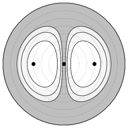
(b)

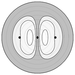
(c)

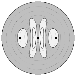
Figure 3: The efficiency of the interferometer’s response to monochromatic gravitational waves at several wavelengths. From top: $\omega_{\text{gw}}2l=$0\text{\,}\rad$$, $3\pi/2\text{\,}\rad$, and $3\pi\text{\,}\rad$. The three filled circles in each plot indicate the orientation of the source and receiving elements. On the left are plots of the efficiency in the plane of the interferometer with the outer ring being an efficiency of 1 and with rings drawn at intervals of 0.1. On the right are the same functions shown as contour plots over the full sky with contours drawn at $-3\text{\,}\mathrm{d}\Bel$, $-6\text{\,}\mathrm{d}\Bel$, and $-9\text{\,}\mathrm{d}\Bel$ relative to the detector’s best possible efficiency of $\epsilon_{\text{max}}\approx 0.65$ (visible as the peak efficiency in the top-leftmost plot).

These show, specifically, the behaviour of the function

$$\epsilon=\frac{1}{2\omega_{\text{gw}}l}\left|(1+\cos\theta)\cos 2\alpha\sin(\omega_{\text{gw}}l\sin\theta\sin\phi)\right|$$

both in the plane of the interferometer, $\phi=\pm\pi/2$ (figures on the left), and over the full sky (figures on the right), for three choices of gravitational wave wavelength: from top to bottom $\omega_{\text{gw}}2l=$0\text{\,}\rad$$, $3\pi/2\text{\,}\rad$, and $3\pi\text{\,}\rad$. In all plots, the polarization of the gravitational wave is chosen so as to maximize the efficiency ($\alpha=$0\text{\,}\rad$$). For the plots of the efficiency in the plane of the interferometer, the scale is such that the outer ring indicates an efficiency of 1 and rings are drawn at intervals of 0.1. The three filled circles indicate the orientation of the interferometer elements with the uppermost circle indicating the direction toward the radio source ($\theta=$0\text{\,}\rad$$). In the full-sky contour plots, the filled circle at the centre of each plot indicates the direction toward the radio source, while the outer ring corresponds to the direction away from the radio source and the two filled circles at $\pi/2\text{\,}\rad$ from the centre indicate the directions toward the receiving elements. Contours are drawn at $-3\text{\,}\mathrm{d}\Bel$, $-6\text{\,}\mathrm{d}\Bel$, and $-9\text{\,}\mathrm{d}\Bel$ relative to the detectors best possible efficiency of $\epsilon_{\text{max}}\approx 0.65$. Several features are noteworthy:

• The direction of greatest sensitivity to gravitational waves is not perpendicular to the interferometer’s lines of sight to the radio source, where one might expect the wave’s polarization to be most favourable, but rather lies in a direction displaced from the perpendicular toward the radio source.

• The interferometer is almost completely insensitive to gravitational waves approaching from directions away from the radio source.

• Compared to the response to longer wavelengths (Figure 3a), the interferometer responds poorly to gravitational waves with wavelengths shorter than the interferometer’s baseline (Figure 3c).

To more clearly see how the frequency response of the interferometer depends on the baseline length, Figure 4 shows the interferometer’s effective length in the direction of greatest sensitivity as a function of the gravitational wave’s angular frequency for three choices of baseline.

Figure 4: The interferometer’s effective length (in the direction of greatest sensitivity) in units of light travel time as it depends on the angular frequency of the gravitational wave and the length of the interferometer’s baseline. For the purpose of illustration, baseline lengths of $2l/c=$1\text{\,}\mathrm{s}$$ (solid curve), $\frac{1}{2}\text{\,}\mathrm{s}$ (long dashes) and $\frac{1}{4}\text{\,}\mathrm{s}$ (short dashes) were chosen. A larger effective length means the generation of a larger differential phase for the same gravitational wave amplitude and thus a more sensitive detector.

For the purpose of illustration, some fairly long baseline lengths were chosen: in terms of the light crossing time, they have lengths of $1\text{\,}\mathrm{s}$, $\frac{1}{2}\text{\,}\mathrm{s}$, and $\frac{1}{4}\text{\,}\mathrm{s}$. The gravitational waves with these wavelengths have angular frequencies of $2\pi\text{\,}\mathrm{rad}\mathrm{/}\mathrm{s}$, $4\pi\text{\,}\mathrm{rad}\mathrm{/}\mathrm{s}$ and $8\pi\text{\,}\mathrm{rad}\mathrm{/}\mathrm{s}$ respectively. Recalling that the effective length is a measure of the sensitivity of the interferometer to gravitational waves, Figure 4 shows a flat response to gravitational waves with wavelengths longer than the interferometer’s baseline. The poor short wavelength performance is attributable to the differential phase being the convolution of the gravitational waveform with a square window whose duration is comparable to the light-crossing time of the interferometer’s baseline: gravitational waves with periods less than this are smoothed out, diminishing their influence on the interferometer’s output. Lest one think the solution to the poor high frequency performance is to use shorter baselines, we also see from Figure 4 that going to shorter baselines does not improve the high frequency response at all. It does flatten the response to higher frequencies but it accomplishes this by reducing the low frequency sensitivity, making it as poor as that at high frequencies. The conclusion is that longer baselines are better: they improve the low frequency response without, in fact, harming the high frequency response. The interferometer’s flat response at low frequencies can be seen analytically by checking that

$$\lim_{\omega_{\text{gw}}l\rightarrow 0}\frac{\,\mathrm{d}\epsilon}{\,\mathrm{d}\omega_{\text{gw}}}=0,$$

and the actual efficiency the interferometer asymptotes to at low frequencies is given by

$$\lim_{\omega_{\text{gw}}l\rightarrow 0}\epsilon=\frac{1}{2}\left|(1+\cos\theta)\sin\theta\sin\phi\cos 2\alpha\right|.$$

It is interesting that although longer baselines do improve the overall sensitivity of the interferometer, contrary to what one might expect upon consideration of Figure 1 it is not necessary to construct an interferometer with a long baseline in order to avoid being insensitive to long wavelength gravitational waves. One might have thought, for example, that a gravitational wave with a wavelength much longer than the separation of the receiving elements would have the two lines of sight always sitting at approximately the same phase within the wave, thus making it difficult to detect its presence. However, the long wavelength also means the gravitational wave’s effect on the radio signal is integrated over a longer segment of the line of sight. The two effects balance each other giving the interferometer a flat response at low frequencies.

Although this section has looked specifically at an exactly monochromatic gravitational wave, the results can be reasonably applied to many anticipated astrophysical sources of gravitational waves. From (22), the relationship between the differential phase and the gravitational waveform only involves the integration of the waveform over an interval roughly equivalent to the light-crossing time of the interferometer’s baseline. The results of this section continue to hold so long as the gravitational wave is approximately monochromatic over this interval. For radio receiving elements restricted to the surface of the Earth, this is an interval less than $40\text{\,}\mathrm{ms}$. Even for space-based antennas separated by millions of kilometres the interval is on the order of $10\text{\,}\mathrm{s}$. Over these time scales, many anticipated astrophysical sources of gravitational waves can be approximated as exactly periodic.

IV.2 Black Hole Ring-Down Gravitational Wave

One example of an astrophysical system that can’t reasonably be approximated as exactly periodic over tens of milliseconds is a perturbed black hole. When a spinning black hole is distorted, the irregularities of its event horizon are radiated away in the form of gravitational waves. The particular waveform generated by this process is called a “black hole ring-down” waveform and is of the form Costa and Aguiar (2003); Echeverria (1989)

$$h(t)=\begin{cases}0,&t<$0\text{\,}\mathrm{s}$,\\ h\mathrm{e}^{-\omega_{\text{s}}t/(2Q)}\sin\omega_{\text{s}}t,&t\geq$0\text{\,}\mathrm{s}$,\end{cases}$$ (29)

where

$$\omega_{\text{s}}\approx($200\text{\,}\mathrm{k}\rad\mathrm{/}\sec$)\left[1-0.63(1-a)^{\frac{3}{10}}\right]\left(\frac{M}{{M}_{\odot}}\right)^{-1}$$ (30)

is the centre frequency of the black hole’s fundamental quadrupolar mode,

$$Q\approx 2(1-a)^{-\frac{9}{20}}$$ (31)

is the “quality factor,” $M/{M}_{\odot}$ is the black hole’s mass in solar mass units, and $a$ is the black hole’s dimensionless angular momentum (it’s physical angular momentum is $aMG/c^{2}$). From (22), the interferometer’s differential phase, $\Delta\phi(t)$, is related to the gravitational waveform by integration over an interval of time. Adjusting the origin of the time co-ordinate in (22) so that this interval just encounters the start of the ring-down waveform at $t=0$, the differential phase produced by this type of wave is

$$\Delta\phi(t)=h\frac{\omega_{\text{r}}}{2}(1+\cos\theta)\cos 2\alpha\,\cdot\\ \int_{t_{\text{start}}}^{t}\mathrm{e}^{-\omega_{\text{s}}\tau/(2Q)}\sin\omega_{\text{s}}\tau\,\mathrm{d}\tau$$

for $t\geq 0$, where

$$t_{\text{start}}=\text{max}(0,t-2l\sin\theta\sin\phi).$$

This evaluates to

$$\Delta\phi(t)=h\frac{\omega_{\text{r}}}{\omega_{\text{s}}}\frac{Q}{1+4Q^{2}}(1+\cos\theta)\cos 2\alpha\,\cdot\\ \left[-\mathrm{e}^{-\omega_{\text{s}}\tau/(2Q)}(2Q\cos\omega_{\text{s}}\tau+\sin\omega_{s}\tau)\right]_{t_{\text{start}}}^{t}.$$ (32)

A detailed exploration of the response of the radio interferometer to the full parameter space of these ring-down gravitational waveforms is outside the scope of this document. To illustrate the nature of the interferometer’s response, we consider the single choice of parameters consisting of $M=50{M}_{\odot}$, and $a=0.3$. Such a black hole’s fundamental quadrupolar mode has a centre frequency of $\omega_{\text{s}}=$1736\text{\,}\mathrm{rad}\mathrm{/}\mathrm{s}$$, and the ring-down waveform has a quality factor of $Q=2.348$. The ring-down waveform is shown in Figure 5.

Figure 5: The ring-down waveform for a black hole of mass $M=50{M}_{\odot}$ and dimensionless angular momentum $a=0.3$.

The interferometer’s response to this type of gravitational wave is depicted in Figure 6 which is a plot of $2\Delta\phi(t)/(h\omega_{\text{r}})$ as a function of time when the gravitational wave is approaching from the optimum direction with the optimum polarization.

Figure 6: The interferometer’s response to the ring-down waveform for two choices of baseline: $6000\text{\,}\mathrm{km}$ (solid curve) and $12000\text{\,}\mathrm{km}$ (dashes). These baselines have light-crossing times of $20\text{\,}\mathrm{ms}$ and $40\text{\,}\mathrm{ms}$ respectively.

For these ring-down waveforms, the output of the interferometer is not proportional to the gravitational wave signal, as it is with monochromatic gravitational waves, so there is no clear way to define a quantity similar to the “effective phase length.” Comparing to the analysis of monochromatic gravitational waves in the previous section, the RMS time average of the function plotted in Figure 6 is algebraically equal to the efficiency times the baseline, $\epsilon 2l$ (hence the choice of milliseconds for the units of the vertical axis). The RMS average over infinite time, however, would give a result of 0, so for gravitational waves localized in time this procedure is not a good way to assess the strength of the interferometer’s output.

The interferometer’s response is plotted for two choices of the interferometer’s baseline: $6000\text{\,}\mathrm{km}$ and $12000\text{\,}\mathrm{km}$ (light crossing times of $20\text{\,}\mathrm{ms}$ and $40\text{\,}\mathrm{ms}$ respectively). The shape of the interferometer’s response as a function of time can be understood as follows. Prior to $t=$0\text{\,}\mathrm{s}$$, the gravitational wave has not yet encountered the interferometer and there is no differential phase seen. At $t=$0\text{\,}\mathrm{s}$$, the ring-down wave train wave crosses the line of sight of the first receiving element, resulting in that station accumulating a phase change in its received radio signal. There is then a constant differential phase between the stations until the wave train crosses the line of sight of the second receiving element (a little less than either $20\text{\,}\mathrm{ms}$ or $40\text{\,}\mathrm{ms}$ later). At that time the second station accumulates the same change in the phase of its received radio signal and the differential phase between the stations returns to 0.

V Noise in the Interferometer

To assess the viability of the type of gravitational wave detector described in this paper, it is necessary to investigate the noise that must be anticipated in the detector’s output. A full analysis of the noise level requires a complete specification not only of the detection apparatus but also of the observation strategies and data analysis techniques to be used in the extraction of a gravitational wave signal from the detector’s raw output.

The technique of gravitational wave detection described in this paper can, in principle, be implemented with both optical and radio technologies. Although it has been implied throughout the document that it is radio systems that are being considered, the analysis up to this point is applicable to both. Optical systems benefit from operation at higher angular frequencies but radio systems, at least terrestrially, benefit from much longer baselines and the ability to record the electromagnetic signals for detailed off-line analysis. Another advantage of the implementation of the detector using radio technology is the possibility of simultaneous multi-use of the technology for other scientific research. We now specifically assume a radio-based system. There will be little discussion of observation strategies or data analysis techniques as these are beyond the scope of this paper.

Gravitational wave detection proves to be one of the most challenging measurement problems in modern physics. All detection techniques currently being used or considered require extraordinary technological achievements. The technique described here does not provide a “magic bullet” for circumventing any of the difficulties in gravitational wave detection so one must expect that the practical implementation of this technique will also require an apparatus with extraordinary operating parameters.

V.1 Thermal Noise in the Electronics

The antenna structures, radio receivers and data acquisition systems used in astronomical radio interferometry applications are not noise-free, and contribute to the uncertainty in the measurement of the interferometer phase. Figure 7 shows an example complex phasor diagram for the radio signal being received and the thermal noise added to it by the interferometer.

Figure 7: Complex signal and noise phasors for the radio signal being received by the interferometer.

If the signal-to-noise ratio is greater than 1, then it can be seen that the phase error introduced by the noise is

$$\delta\phi\sim\frac{\left|\text{noise}\right|}{\left|\text{signal}\right|}=\text{SNR}_{\text{r}}^{-1}$$

where the subscript r on the right-hand side identifies this as the radio interferometer’s signal-to-noise ratio. If we take our gravitational wave signal to be the time-averaged RMS differential phase in (27a) and compare this to the phase noise from above, we get

$$\text{SNR}_{\text{gw}}=\frac{\Delta{\phi}_{\text{rms}}}{\delta\phi}=\Delta{\phi}_{\text{rms}}\,\text{SNR}_{\text{r}}$$

as the signal-to-noise ratio on a single determination of the differential phase due to the presence of a gravitational wave. Since $\Delta{\phi}_{\text{rms}}\propto h\frac{\omega_{\text{r}}}{\omega_{\text{gw}}}$ is typically much smaller than 1, we see immediately that we are going to need a very high signal-to-noise ratio in the interferometer in order to see gravitational waves above the thermal noise.

The signal-to-noise ratio of a two-element radio interferometer is given by (Thompson et al., 1991, page 158)

$$\text{SNR}_{\text{r}}=\frac{1}{\sqrt{2\pi}}\sqrt{\Delta\omega_{\text{r}}\Delta t}\sqrt{\frac{{T_{\text{A}}}_{1}{T_{\text{A}}}_{2}}{{T_{\text{sys}}}_{1}{T_{\text{sys}}}_{2}}}$$

where $\Delta\omega_{\text{r}}/(2\pi)$ is the bandwidth of the receiving system in Hertz, $\Delta t$ is the coherent integration time in seconds, ${T_{\text{A}}}_{i}$ is the antenna (signal) temperature in Kelvin at the $i^{\text{th}}$ antenna, and ${T_{\text{sys}}}_{i}$ is the system (noise) temperature in Kelvin at the $i^{\text{th}}$ antenna. The antenna temperature is given by Kraus (1966)

$$T_{\text{A}}=\frac{10^{-26}S_{\nu}A_{\text{eff}}}{2k_{\text{B}}}$$

where $S_{\nu}$ is the spectral flux density of the observed radio source in Janskys ($$1\text{\,}\jansky$=$10^{-26}\text{\,}\mathrm{W}\mathrm{m}^{-2}\mathrm{Hz}^{-1}$$), $A_{\text{eff}}$ is the antenna’s effective aperture area in square metres, and $k_{\text{B}}=$1.4\times 10^{-23}\text{\,}\mathrm{J}\mathrm{K}^{-1}$$ is the Boltzmann constant. The factor of 2 is due to the radio receiver being able to observe only one electromagnetic polarization. For a “blind search” observation of gravitational waves with an angular frequency of $\omega_{\text{gw}}$, our interferometer’s coherent integration time cannot exceed the inverse Nyquist frequency of $\Delta t=\pi/\omega_{\text{gw}}$. If we, further, assume the two receiving stations are identical (same effective apertures, same system temperatures), then altogether the phase uncertainty due to thermal noise in the radio interferometer’s electronics is

$$\delta\phi_{\text{r}}\approx 4\times 10^{3}\sqrt{\frac{\omega_{\text{gw}}}{\Delta\omega_{\text{r}}}}\frac{T_{\text{sys}}}{S_{\nu}A_{\text{eff}}}$$ (33)

where $S_{\nu}$ is in $\jansky$, $T_{\text{sys}}$ is in $\mathrm{K}$, and $A_{\text{eff}}$ is in $\mathrm{m}^{2}$.

V.2 Other Noise Sources

The thermal noise in the interferometer’s electronics limits one’s ability to measure with precision the difference in phase between the signals being received at each station. Even given an exact measurement of the interferometer’s differential phase, it is still difficult to attribute it exclusively to a passing gravitational wave as there are other processes that contribute to phase differences between the receiving stations. Examples of such systematic noise sources are:

• Time-dependant deformations of the interferometer due to, for example, seismic noise and tidal distortion of the Earth.

• Variations in the refractive index of the medium through which the radio waves travel on their way to the receiving stations. These include variations in the refractive index of the Earth’s atmosphere as well as possibly interplanetary or interstellar gases (depending on the distance to the radio source).

• Thermal distortions of the antennas and the consequent displacement of the antenna phase centres.

• Variations in the instrumental signal delays through cables and electronics at each antenna site.

These noise sources, as well as others not mentioned here, affect present day radio astronomical and geodetic radio interferometric observations. In general it will be necessary to either remove the effects of systematic noise sources by clever observing strategies and/or sophisticated signal processing techniques, or to provide calibration systems that are capable of accounting for their presence. In some cases, present-day radio interferometric techniques may be capable of providing the necessary tools. For example, dispersive effects of the ionosphere and the interplanetary/interstellar medium can be removed by multi-frequency observations and radio interferometry phase calibration (pcal) systems (Thompson et al., 1991, page 290) can remove the effects of variations in instrumental phase delay between stations at the picosecond level Cannon .

Differential observing strategies may possibly be developed that are effective in removing systematic effects in the output data. Figure 3 shows that, as a gravitational wave detector, a radio interferometer is reasonably directional, and the use of antenna arrays and beam-forming techniques might be employed to implement a gravitational wave detector with high directivity. Such a system combined with multi-beam radio frequency antennas could, in principle, carry out a differential search for gravitational waves incident from several directions on the sky simultaneously. Differential observing strategies such as this are capable of cancelling systematic noise sources to a high precision.

The sources of noise mentioned above produce differential phase in the interferometer through means other than the curvature of space. Even when all such noise can be removed from the interferometer’s output, leaving only curvature-induced differential phase, there are sources of curvature other than gravitational waves. Phenomena such as seismic and atmospheric activity can produce changes in local gravity comparable to the expected amplitude of astrophysical gravitational waves Schutz (1999). Unlike ground-based laser interferometers, the radio signals used by the type of detector investigated here do not travel along geodesics that are entirely local to the Earth. For this reason, it is not yet clear the extent to which such sources of noise contribute to the detector’s output but it is possible this type of detector is less sensitive to them than are entirely ground-based systems.

A full analysis of the noise from these and other sources and the extent to which these can be subtracted from the detector’s output will be the subject of future work.

VI Practical Gravitational Wave Detection

If we assume for the moment that all systematic sources of differential phase can be exactly accounted for and subtracted from the detector’s output, then that leaves the interferometer’s thermal noise as the only impediment to the operation of this type of detector. While this is an unrealistic situation, it does represent a sensitivity limit which cannot be improved upon through any amount of creative observation strategies or signal extraction techniques (with the exception of extending the interferometer’s integration time, and this will be discussed below).

For good gravitational wave signal to noise, it has been established that long baselines, high frequency radio observations, low receiver noise temperatures and bright radio sources are required. In addition, one can consider performing multiple simultaneous observations of a gravitational wave: by constructing an interferometer with more than two elements, the differential phase across multiple baselines can be measured. If these measurements are time-shifted appropriately and summed together, the thermal noise in the individual measurements will sum incoherently while any signal that is present will be summed coherently. For $N$ baselines, the relative phase noise could be reduced by as much as a factor of $\sqrt{N}$.

Setting $\Delta{\phi}_{\text{rms}}$ in (27a) equal to $\delta\phi_{\text{r}}$ in (33) and solving for $h$ gives us the gravitational wave shear needed to achieve a signal-to-noise ratio of at least 1. This is

$$h_{\text{min}}=6\times 10^{3}\sqrt{\frac{\omega_{\text{gw}}^{3}}{\omega_{\text{r}}^{2}\Delta\omega_{\text{r}}}}\frac{T_{\text{sys}}}{S_{\nu}A_{\text{eff}}}\,\cdot\\ \left|(1+\cos\theta)\cos 2\alpha\sin(\omega_{\text{gw}}l\sin\theta\sin\phi)\right|^{-1}.$$ (34)

Optimistic yet achievable numbers for some of the parameters in this expression are: a radio observation centre frequency of $\omega_{\text{r}}=$10^{11}\text{\,}\mathrm{rad}\mathrm{/}\mathrm{s}$$, a bandwidth of $\Delta\omega_{\text{r}}=$10^{9}\text{\,}\mathrm{rad}\mathrm{/}\mathrm{s}$$, system temperatures of $T_{\text{sys}}=$20\text{\,}\mathrm{K}$$, effective apertures of $A_{\text{eff}}=$10^{3}\text{\,}\mathrm{m}^{2}$$, and an interferometer consisting of 32 stations for a total of 496 baselines of about $2l=$2000\text{\,}\mathrm{km}$$ ($l=$3\text{\,}\mathrm{ms}$$) each. Given these parameters, Figure 8 shows plots of $h_{\text{min}}$ for radio source spectral flux densities of $10^{2}\text{\,}\jansky$ and $10^{4}\text{\,}\jansky$ (at $16\text{\,}\mathrm{GHz}$).

Figure 8: The minimum shear required in order to achieve a signal to noise ratio of 1 in the observation of gravitational waves using a radio interferometer array with the parameters listed in the text. Two radio source spectral flux densities are considered: $10^{2}\text{\,}\jansky$ (solid line) and $10^{4}\text{\,}\jansky$ (dashed line). Compare to Figure 4 of Cutler and Thorne (2002).

Flux densities of this order are available naturally from galactic water vapour maser sources at $22\text{\,}\mathrm{GHz}$ or could be provided artificially, for example by means of a spacecraft-born radio transmitter. The Canadian Large Adaptive Reflector (CLAR), embodies a design for a low-cost, large aperture ($300\text{\,}\mathrm{m}$ diameter or larger), fully-steerable, multi-beam radio astronomy antenna Côté et al. (2002); Dewdney (2000); Cannon (1996). One technical implementation for the Square Kilometre Array (SKA) envisages the construction of an array of CLAR antennas. Such an interferometer array might, potentially, have use in the search for gravitational radiation although its anticipated operating parameters differ somewhat from the numbers quoted above.

To compare the sensitivity of this type of detector to those of other types, as well as to the strengths of anticipated sources of gravitational waves, see the recent reviews found in Cutler and Thorne (2002) and Schutz (1999). The noise curves in Figure 8 are well above any anticipated gravitational wave signals. It must be recalled, however, that these noise curves are for the raw detection of a gravitational wave signal at or above the noise level: a pen on a chart recorder marking out the gravitational wave shear as a function of time. This picture is not what is meant when it is said that the current generation of gravitational wave observatories will “observe” gravitational waves. Rather than obtaining a direct read-out of the gravitational wave shear as a function of time, one convolves the output of the detector against a template waveform and compares the correlation coefficient to a baseline coefficient obtained by correlating the same template against a model of the detector’s noise. By this method, one extends the coherent integration time of the interferometer and reduces the output to the probability that the given waveform is present in the data. In the case of many astrophysical sources, such as binary neutron star systems, integration times of months or even years are anticipated Finn and Thorne (2000). This is to be contrasted to the integration times of $\leq$10^{3}\text{\,}\mathrm{s}$$ that were assumed for the computation of Figure 8. Since the noise curves in Figure 8 are inversely proportional to the square root of the integration time, then if such long integration times could be used in the radio interferometer one could potentially decrease $h_{\text{min}}$ by two or three orders of magnitude. In the frequency band shown in Figure 8, such a reduction in the noise levels would make this type of detector competitive with the LISA detector’s noise level as shown in Figure 4 of Cutler and Thorne (2002).

It must be stressed, however, that systematic noise has been ignored. An analysis of the contribution from systematic noise is complicated by the availability of sophisticated calibration techniques that can subtract a great deal of it. A complete analysis of the influence of systematic noise will involve not only an estimate of the raw contribution from these sources but also the development and subsequent analysis of the effectiveness of observation strategies and data processing techniques. This will be the subject of future work.

VII Conclusions

The technique, introduced here, of using the time-dependent phase difference between two radio receiving stations to watch for the passage of a gravitational wave would seem to be a promising method of gravitational wave observation worthy of further investigation. In the future, a more detailed analysis of realistic interferometer configurations and data analysis techniques will shed more light on true sensitivity of this type of detector.

References

- Caron et al. (1997) B. Caron, A. Dominjon, C. Drezen, R. Flaminio, X. Grave, F. Marion, L. Massonnet, C. Mehmel, R. Morand, B. Mours, et al., Classical and Quantum Gravity 14, 1461 (1997).
- Danzmann (1997) K. Danzmann, Classical and Quantum Gravity 14, 1399 (1997).
- Lück and the GEO600 Team (1997) H. Lück and the GEO600 Team, Classical and Quantum Gravity 14, 1471 (1997).
- Kawabe and the TAMA collaboration (1997) K. Kawabe and the TAMA collaboration, Classical and Quantum Gravity 14, 1471 (1997).
- Abramovici et al. (1992) A. Abramovici, W. E. Althouse, R. W. P. Drever, Y. Gürsel, S. Kawamura, F. J. Raab, D. Shoemaker, L. Sievers, R. E. Spero, K. S. Thorne, et al., Science 256, 325 (1992).
- Ni (2002) W.-T. Ni, International Journal of Modern Physics D 11, 947 (2002).
- Bertotti et al. (1998) B. Bertotti, A. Vecchio, and L. Iess (1998), and references therein, eprint arXiv:gr-qc/9806021.
- Hellings (1986) R. W. Hellings, Astronomical Journal 91, 650 (1986).
- Schutz (1999) B. F. Schutz, Classical and Quantum Gravity 16, A131 (1999), eprint arXiv:gr-qc/9911034.
- Costa and Aguiar (2003) C. A. Costa and O. D. Aguiar (2003), eprint arXiv:gr-qc/0309047.
- Echeverria (1989) F. Echeverria, Physical Review D 40, 3194 (1989).
- Thompson et al. (1991) A. R. Thompson, J. M. Moran, and G. W. Swenson, Interferometry and Synthesis in Radio Astronomy (Krieger Publishing, 1991), 2nd ed.
- Kraus (1966) J. D. Kraus, Radio Astronomy (McGraw-Hill Book Company, Inc., 1966), 1st ed.
- (14) W. H. Cannon, personal communication.
- Cutler and Thorne (2002) C. Cutler and K. S. Thorne (2002), eprint arXiv:gr-qc/0204090.
- Dewdney (2000) P. Dewdney (2000), talk given at the Jodrell Bank SKA Workshop.
- Côté et al. (2002) S. Côté, A. R. Taylor, and P. E. Dewdney (2002), eprint arXiv:astro-ph/0204323.
- Cannon (1996) K. C. Cannon, Tech. Rep., Space Geodynamics Laboratory, Institute for Space And Terrestrial Science, Toronto (1996).
- Finn and Thorne (2000) L. S. Finn and K. S. Thorne, Physical Review D 62 (2000), eprint arXiv:gr-qc/0007074.