Ultra-high-precision velocity measurements of oscillations in $\alpha$ Cen A

Abstract

We have made differential radial velocity measurements of the star $\alpha$ Cen A using two spectrographs, UVES and UCLES, both with iodine absorption cells for wavelength referencing. Stellar oscillations are clearly visible in the time series. After removing jumps and slow trends in the data, we show that the precision of the velocity measurements per minute of observing time is 0.42 m s^-1 for UVES and 1.0 m s^-1 for UCLES, while the noise level in the Fourier spectrum of the combined data is 1.9 cm s^-1. As such, these observations represent the most precise velocities ever measured on any star apart from the Sun.

1 Introduction

The search for extra-solar planets has driven tremendous improvements in high-precision measurements of stellar differential radial velocities (e.g., Marcy & Butler, 2000). In parallel, the same techniques have been used with great success to measure stellar oscillations. Recent achievements, reviewed by Bouchy & Carrier (2003) and Bedding & Kjeldsen (2003), include observations of oscillations in Procyon with ELODIE (Martic et al., 1999, see also Barban et al., 1999); $\beta$ Hyi with UCLES (Bedding et al., 2001) and CORALIE (Carrier et al., 2001); and $\alpha$ Cen A and B with CORALIE (Bouchy & Carrier, 2001, 2002; Carrier & Bourban, 2003). Here we report observations of $\alpha$ Cen A made with UVES and UCLES which represent the most precise differential radial velocities ever measured on any star apart from the Sun.

2 Observations

We observed $\alpha$ Cen A in May 2001 from two sites. At the European Southern Observatory in Chile we used UVES (UV-Visual Echelle Spectrograph) at the 8.2-m Unit Telescope 2 of the Very Large Telescope (VLT). At Siding Spring Observatory in Australia we used UCLES (University College London Echelle Spectrograph) at the 3.9-m Anglo-Australian Telescope (AAT). In both cases, an iodine cell was used to provide a stable wavelength reference (Butler et al., 1996).

At the VLT we obtained 3013 spectra of $\alpha$ Cen A, with typical exposure times of 1–3 s and a median cadence of one exposure every 26 s. At the AAT we obtained 5169 spectra of $\alpha$ Cen A, with typical exposure times of 6 s and a median cadence of one exposure every 20 s. The resulting velocities are shown in Fig. 1, and the effects of bad weather can be seen (we were allocated four nights with the VLT and six with the AAT).

The UCLES velocities show upward trends during most nights, which we believe to be related to the slow movement of the CCD dewar as liquid nitrogen boiled off. Nights three and (particularly) five also show a jump that coincides with the refilling of the CCD dewar in the middle of the night. These UCLES observations differed from our earlier run on $\beta$ Hyi (Bedding et al., 2001), and also from standard UCLES planet-search observations, in that the CCD was rotated by 90 degrees to speed up readout time. This had the side-effect of causing the CCD readout to be in the same direction as the dispersion, and also of making this direction vertical (so that flexure in the dewar due to changes in its weight would have shifted the spectrum in the dispersion direction). It seems there was an effect on the velocities that was not completely corrected by the iodine reference method, which suggests that either the PSF description or the spectrum extraction from the CCD images was inadequate. We note that improvements to the PSF description are an active area of work to enhance immunity to spectrometer changes. The UVES data, meanwhile, show slow trends and two smaller jumps which are presumably also instrumental – at least one of the jumps can be identified with a correction to the position of the star on the slit. While these jumps and slow trends would seriously compromise a planet search, they fortunately have neglible effect on our measurement of oscillations.

To remove the slow trends, we have subtracted a smoothed version of the data, and this was done separately on either side of the jumps so that they, too, were removed. The detrended time series are shown in Fig. 1. We have verified by calculating power spectra that this process of high-pass filtering effectively removes all power below about 0.2 mHz. It also removes any power at higher frequencies that arises from the jumps, which would otherwise degrade the oscillation spectrum.

3 Analysis and discussion

The time series of velocity measurements clearly show oscillations and the effects of beating between modes (Fig. 2). The data presented here have unprecedented precision and we are interested in obtaining the lowest possible noise in the power spectrum so as to measure as many modes as possible. We also wish to estimate the actual precision of the Doppler measurements.

The algorithm used to extract the Doppler velocity from each spectrum also provides us with an estimate $\sigma_{i}$ of the uncertainty in this velocity measurement. These are derived from the scatter of velocities measured from many small ($\sim 1.7\,$Å) segments of the echelle spectrum. In the past, we have used these values to generate weights ($w_{i}=1/\sigma_{i}^{2}$) for the Fourier analysis (Bedding et al., 2001; Kjeldsen et al., 2003). In the present analysis, we take the opportunity to verify that these $\sigma_{i}$ do indeed reflect the actual noise properties of the velocity measurements.

Our first step in this process was to measure the noise in the power spectrum at high frequencies, well beyond the stellar signal. It soon became clear that this procedure implied a measurement precision significantly worse than is indicated by the point-to-point scatter in the time series itself. The implication is that some fraction of the velocity measurements are ‘bad,’ contributing a disproportionate amount of power in Fourier space.

Since the oscillation signal is the dominant cause of variations in the velocity series, we need to remove this signal in order to estimate the noise and to locate the bad points. We chose to remove the signal iteratively by finding the strongest peak in the power spectrum and subtracting the corresponding sinusoid from the time series. This procedure was carried out for the strongest peaks in the oscillation spectrum in the frequency range 0–3.5 mHz, until spectral leakage into high frequencies from the remaining power was negligible. We were left with a time series of residual velocities, $r_{i}$, which reflects the noise properties of the measurements.

The next step was to analyse the residuals for evidence of bad points, which we would recognize as those values deviating from zero by more than would be expected from their uncertainties. In other words, we examined the ratio $r_{i}/\sigma_{i}$, which we expect to be Gaussian distributed, so that outliers correspond to suspect data points. We found that the best way to investigate this was via the cumulative histogram of $|r_{i}/\sigma_{i}|$, which is shown for both the UVES and UCLES as the points in the upper panels of Fig. 3. The solid curves in these figures show the cumulative histograms for the best-fitting Gaussian distributions. We indeed see a significant excess of outliers for $|r_{i}/\sigma_{i}|$ beyond about 2, in both data sets. The lower panels show the ratio between the points and the curve, which is the fraction $f$ of data points that could be considered as good. This fraction is essentially unity out to $|r_{i}/\sigma_{i}|\simeq 2$, and then falls off, indicating that about half the data points with $|r_{i}/\sigma_{i}|>3$ are bad.

At this point, we could simply make the decision to ignore all data points with $|r_{i}/\sigma_{i}|$ above a certain value, such as 3.0, on the basis that many of them would be bad points that would increase the noise in the oscillation spectrum. We instead chose a more elegant approach, which gave essentially the same results, in which we used the information in Fig. 3 to adjust the weights: those points with large values of $|r_{i}/\sigma_{i}|$ were decreased in weight, with every $w_{i}$ multiplied by the factor $f$. Given that the weights are calculated as $w_{i}=1/\sigma_{i}^{2}$, the adjustment was achieved by dividing each measurement error ($\sigma_{i}$) by the square root of $f$.

With these adjustments to the measurement uncertainties, which effectively down-weight the bad data points, we now expect the noise floor at high frequencies in the amplitude spectrum of the residuals ($r_{i}$) to be substantially reduced. We measured the average noise $\sigma_{\rm amp}$ in the range 7.5–15 mHz to be 2.11 cm s^-1 for UVES and 4.37 cm s^-1 for UCLES. The corresponding values before down-weighting the bad data points were 2.33 cm s^-1 for UVES and 4.99 cm s^-1 for UCLES. We can therefore see that adjusting the weights has lowered the noise by about 10%.

The final stage in this processing involved checking the calibration of the uncertainties. By this, we mean that the estimates $\sigma_{i}$ should be consistent with the noise level determined from the amplitude spectrum. On the one hand, the mean variance of the data can be calculated as a weighted mean of the $\sigma_{i}$, as follows:

$$\sum_{i=1}^{N}\sigma_{i}^{2}w_{i}\left/\sum_{i=1}^{N}w_{i}\right.,$$ (1)

where the weights are given by $w_{i}=1/\sigma_{i}^{2}$ (which means the numerator is simply equal to $N$). On the other hand, the variance deduced from the noise level $\sigma_{\rm amp}$ in the amplitude spectrum is (Appendix A.1 of Kjeldsen & Bedding, 1995):

$$\sigma_{\rm amp}^{2}N/\pi.$$ (2)

We require these to be equal, which gives the condition

$$\sigma_{\rm amp}^{2}\sum_{i=1}^{N}\sigma_{i}^{-2}=\pi.$$ (3)

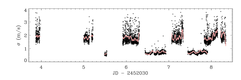
Figure 4: Points show measurement errors in each time series, while the (red) curves show the smoothed residuals (see text)

Using the values of $\sigma_{\rm amp}$ given above, we concluded that Eq. (3) would be satisfied for each data set provided the uncertainties $\sigma_{i}$ were multiplied by 0.78 for UVES and 0.87 for UCLES. It is these calibrated $\sigma_{i}$ that are shown in Figs. 2 and 4, and they represent our best estimate of the high-frequency precision of the data. Also shown in Fig. 4 as solid lines are the residuals $r_{i}$ after smoothing with a running box-car mean. We can see that there is generally very good agreement between these two independent measures of the velocity precision, giving us confidence that we have correctly estimated $\sigma_{i}$ both in relative terms and in the absolute calibration.

We have also investigated the dependence of the velocity precision on the photon flux in the stellar spectrum. Figure 5 shows $\sigma_{i}$ versus the signal-to-noise ratio (SNR), where the latter is the square root of the median number of photons per pixel in the iodine region of the spectrum. The points for both UVES and UCLES agree well with a slope of $-1$ in the logarithm, as expected for Poisson statistics. We also note that the offset between the two sets of points arises because of the difference in dispersion of the spectrographs. UVES has higher dispersion, by a factor of 1.55, which means that not only is velocity precision expected to be better by this factor, but also that the SNR per unit wavelength is lower (by the square root of this factor). Combining these effects, we would expect the two distributions to be in the ratio $1.55^{1.5}=1.93$, which is exactly what we find in Fig. 5. In other words, the lower precision in the UVES data at a given SNR per pixel results from the higher dispersion but, allowing for this, the intrinsic precision is the same for the two systems. In addition, the CCD on the UVES system was able to record more photons per exposure than UCLES (the median SNR is considerably higher).

The result of the processing described above was a time series for both UVES and UCLES, each of which consisted of the time stamps, the measured velocities (after correction for jumps and drifts) and the uncertainty estimates (after the adjustments described). These two time series could then be merged in order to produce the oscillation power spectrum, and this is shown in Fig. 6. The average noise in the amplitude spectrum in the range 7.5–15 mHz is 2.03 cm s^-1. As discussed at the beginning of this section, some of this power comes from spectral leakage of the oscillation signal itself. Therefore, a more accurate measure of the noise is obtained from the power spectrum of the residuals, $r_{i}$, when using the final weights, $1/\sigma_{i}^{2}$. The result gives an average noise in the range 7.5–15 mHz of 1.91 cm s^-1. For comparison, the noise level reported from CORALIE observations of $\alpha$ Cen A was 4.3 cm s^-1 (Bouchy & Carrier, 2002), while observations of $\alpha$ Cen B gave 3.75 cm s^-1 (Carrier & Bourban, 2003).

We can also calculate the precision per minute of observing time, which is shown in Table 1. For comparison, we include velocity precision from other oscillation measurements. The list is not meant to be exhaustive, but most of the instruments that have been used in recent years are represented. The precision depends, of course, on several factors such as the telescope aperture, target brightness, observing duty cycle, spectrograph stability and method of wavelength calibration. It is clear that the observations reported here, particularly those with UVES, are significantly more precise than any previous measurements of stars other than the Sun. Of course, we refer here to the precision at frequencies above $\sim 0.8$ mHz, which is the regime of interest for oscillations in solar-type stars.

The referee has questioned whether adjusting the weights using the method described above might have affected the accuracy with which the oscillation frequencies can be measured. To test this, we have extracted the ten highest peaks from both the power spectrum in Fig. 6 and from the power spectrum obtained without adjusting the weights. The frequencies of all ten peaks agreed very well, with a mean difference of 0.11 $\mu$Hz and a maximum difference of 0.4 $\mu$Hz. The latter is a factor of ten smaller than the FWHM of the spectral window and probably well below the natural linewidth of the modes. Therefore, there is no reason to think that the reduction in the noise level obtained by adjusting weights has come at the expense of reduced accuracy in the measured frequencies.

4 Conclusion

We have analysed differential radial velocity measurements of $\alpha$ Cen A made with UVES at the VLT and UCLES at the AAT. Stellar oscillations are clearly visible in the time series. Slow drifts and sudden jumps of a few metres per second, presumably instrumental, were removed from each time series using a high-pass filter. We then used the measurement uncertainties as weights in calculating the power spectrum, but we found it necessary to modify some of the weights to account for a small fraction of bad data points. In the end, we reached a noise floor of 1.9 cm s^-1 in the amplitude spectrum and in a future paper we will present a full analysis of the oscillation frequencies and a comparison with stellar models.

Figure 1: Time series of velocity measurements of $\alpha$ Cen A, both before and after removal of jumps and slow trends. The times of the jumps in UVES are at 6.655 and 6.760, and those for UCLES are at 6.122 and 8.110.

Figure 2: A four-hour segment of the detrended UVES velocity time series, showing 1-$\sigma$ error bars.

Figure 3: Upper: cumulative histograms of $|r_{i}/\sigma_{i}|$ for UVES (left) and UCLES) right. The points show the observations and the solid curve shows the result expected for Gaussian-distributed noise. Lower: the ratio between observed and expected histograms, indicating the fraction of “good” data points.

Figure 5: Measurement errors as a function of SNR. The two straight lines both have slopes of $-1$, and are displaced from each other by a factor 1.93 (see text).

Figure 6: Power spectrum of the combined velocity time series. The inset shows the spectral window, with the frequency scale expanded by a factor of ten.

Table 1: Noise levels from observations of solar-like oscillations

Star	Spectrograph	Precision in	Reference
		1 min (m s-1)
Sun	BiSON	0.2	data supplied by W. Chaplin
$\alpha$ Cen A	UVES	0.42	this paper
Sun	GOLF	0.6	data from the GOLF Web site
$\alpha$ Cen A	UCLES	1.0	this paper
$\alpha$ Cen B	CORALIE	1.7	Carrier & Bourban (2003)
$\alpha$ Cen A	CORALIE	1.7	Bouchy & Carrier (2002)
Procyon	ELODIE	2.5	Martic et al. (1999)
Procyon	CORALIE	2.7	Carrier et al. (2002)
$\beta$ Hyi	UCLES	3.0	Bedding et al. (2001)
$\beta$ Hyi	CORALIE	4.2	Carrier et al. (2001)
Procyon	AFOE	4.2	Brown (2000)
Procyon	FOE	4.7	Brown et al. (1991)
Procyon	HIDES	5.1	Kambe et al. (2003)

References

- Barban et al. (1999) Barban, C., Michel, E., Martic, M., Schmitt, J., Lebrun, J. C., Baglin, A., & Bertaux, J. L., 1999, A&A, 350, 617.
- Bedding et al. (2001) Bedding, T. R., Butler, R. P., Kjeldsen, H., Baldry, I. K., O’Toole, S. J., Tinney, C. G., Marcy, G. W., Kienzle, F., & Carrier, F., 2001, ApJ, 549, L105.
- Bedding & Kjeldsen (2003) Bedding, T. R., & Kjeldsen, H., 2003, Proc. Astron. Soc. Aust., 20, 203.
- Bouchy & Carrier (2001) Bouchy, F., & Carrier, F., 2001, A&A, 374, L5.
- Bouchy & Carrier (2002) Bouchy, F., & Carrier, F., 2002, A&A, 390, 205.
- Bouchy & Carrier (2003) Bouchy, F., & Carrier, F., 2003, Ap&SS, 284, 21.
- Brown (2000) Brown, T. M., 2000, In Teixeira, T., & Bedding, T. R., editors, The Third MONS Workshop: Science Preparation and Target Selection, page 1. Aarhus: Aarhus Universitet. available via the ADS.
- Brown et al. (1991) Brown, T. M., Gilliland, R. L., Noyes, R. W., & Ramsey, L. W., 1991, ApJ, 368, 599.
- Butler et al. (1996) Butler, R. P., Marcy, G. W., Williams, E., McCarthy, C., Dosanjh, P., & Vogt, S. S., 1996, PASP, 108, 500.
- Carrier et al. (2001) Carrier, F., Bouchy, F., Kienzle, F., Bedding, T. R., Kjeldsen, H., Butler, R. P., Baldry, I. K., O’Toole, S. J., Tinney, C. G., & Marcy, G. W., 2001, A&A, 378, 142.
- Carrier et al. (2002) Carrier, F., Bouchy, F., Kienzle, F., & Blecha, A., 2002, In Aerts, C., Bedding, T. R., & Christensen-Dalsgaard, J., editors, IAU Colloqium 185: Radial and Nonradial Pulsations as Probes of Stellar Physics, volume 259, page 468. ASP Conf. Ser.
- Carrier & Bourban (2003) Carrier, F., & Bourban, G., 2003, A&A, 406, L23.
- Kambe et al. (2003) Kambe, E., Sato, B., Takeda, Y., Izumiura, H., Masuda, S., & Ando, H., 2003, In Thompson, M. J., Cunha, M. S., & Monteiro, M. J. P. F. G., editors, Asteroseismology Across the HR Diagram, page P331. Kluwer.
- Kjeldsen & Bedding (1995) Kjeldsen, H., & Bedding, T. R., 1995, A&A, 293, 87.
- Kjeldsen et al. (2003) Kjeldsen, H., Bedding, T. R., Baldry, I. K., Bruntt, H., Butler, R. P., Fischer, D. A., Frandsen, S., Gates, E. L., Grundahl, F., Lang, K., Marcy, G. W., Misch, A., & Vogt, S. S., 2003, AJ, 126, 1483.
- Marcy & Butler (2000) Marcy, G. W., & Butler, R. P., 2000, PASP, 112, 137.
- Martic et al. (1999) Martic, M., Schmitt, J., Lebrun, J.-C., Barban, C., Connes, P., Bouchy, F., Michel, E., Baglin, A., Appourchaux, T., & Bertaux, J.-L., 1999, A&A, 351, 993.