3D Spectrophotometry of Planetary Nebulae in the Bulge of M31

Martin M. Roth¹¹affiliation: Visiting Astronomer, German-Spanish Astronomical Centre, Calar Alto, operated by the Max-Planck-Institute for Astronomy, Heidelberg, jointly with the Spanish National Commission for Astronomy. ²²affiliation: Visiting Astronomer, Special Astrophysical Observatory, Selentchuk, Russia. , Thomas Becker¹¹affiliation: Visiting Astronomer, German-Spanish Astronomical Centre, Calar Alto, operated by the Max-Planck-Institute for Astronomy, Heidelberg, jointly with the Spanish National Commission for Astronomy. ²²affiliation: Visiting Astronomer, Special Astrophysical Observatory, Selentchuk, Russia. , Andreas Kelz ¹¹affiliation: Visiting Astronomer, German-Spanish Astronomical Centre, Calar Alto, operated by the Max-Planck-Institute for Astronomy, Heidelberg, jointly with the Spanish National Commission for Astronomy. Astrophysikalisches Institut Potsdam, An der Sternwarte 16, D-14482 Potsdam, Germany mmroth@aip.de Jürgen Schmoll¹¹affiliation: Visiting Astronomer, German-Spanish Astronomical Centre, Calar Alto, operated by the Max-Planck-Institute for Astronomy, Heidelberg, jointly with the Spanish National Commission for Astronomy. ²²affiliation: Visiting Astronomer, Special Astrophysical Observatory, Selentchuk, Russia. ³³affiliation: Visiting Astronomer, Isaac Newton Group of Telescopes, La Palma. Astronomical Instrument Group, Dept. of Physics, University of Durham,
Rochester Buildg., South Road, Durham DH1 3LE, United Kingdom Jurgen.Schmoll@durham.ac.uk

Abstract

We introduce crowded field integral field (3D) spectrophotometry as a useful technique for the study of resolved stellar populations in nearby galaxies. The spectroscopy of individual extragalactic stars, which is now feasible with efficient instruments and large telescopes, is confronted with the observational challenge of accurately subtracting the bright, spatially and wavelength-dependent non-uniform background of the underlying galaxy. As a methodological test, we present a pilot study with selected extragalactic planetary nebulae (XPN) in the bulge of M31, demonstrating how 3D spectroscopy is able to improve the limited accuracy of background subtraction which one would normally obtain with classical slit spectroscopy. It is shown that due to the absence of slit effects, 3D is a most suitable technique for spectrophometry. We present spectra and line intensities for 5 XPN in M31, obtained with the MPFS instrument at the Russian 6m BTA, INTEGRAL at the WHT, and with PMAS at the Calar Alto 3.5m Telescope. The results for two of our targets, for which data are available in the literature, are compared with previously published emission line intensities. The three remaining PN have been observed spectroscopically for the first time. One object is shown to be a previously misidentified supernova remnant. Our monochromatic H_α maps are compared with direct Fabry-Pérot and narrowband filter images of the bulge of M31, verifying the presence of filamentary emission of the interstellar medium in the vicinity of our objects. We present an example of a flux calibrated and continuum-subtracted filament spectrum and demonstrate how the ISM component introduces systematic errors in the measurement of faint diagnostic PN emission lines when conventional observing techniques are employed. It is shown how these errors can be eliminated with 3D spectroscopy, using the full 2-dimensional spatial information and point spread function (PSF) fitting techniques. Using 3D spectra of bright standard stars, we demonstrate that the PSF is sampled with high accuracy, providing a centroiding precision at the milli-arcsec level. Crowded field 3D spectrophotometry and the use of PSF fitting techniques is suggested as the method of choice for a number of similar observational problems, including luminous stars in nearby galaxies, supernovae, QSO host galaxies, gravitationally lensed QSOs, and others.

planetary nebulae: extragalactic — galaxies: individual, resolved stellar populations — spectroscopy: 3D, integral field, crowded field — spectrophotometry: 3D

^†^†slugcomment: accepted for publication in The Astrophysical Journal

1 Introduction

Understanding the formation and evolution of galaxies is one of the most prominent goals of modern cosmology. After a long-lasting discussion about the best evolutionary scenarios for elliptical galaxies, for example, either according to the classical picture of instantaneous dissipative collapse (Larson 1974), or rather in the hierarchical scenario through gradual mergers of spirals (White 1980), it seems today that the latter view is the more widely accepted one. The observational evidence, that nearby ellipticals show peculiarities like counter-rotating cores, rings, gas disks, and recent star formation, can be explained by merger and accretion processes over an extended period of time. On the theoretical side, numerical N-body simulations combined with the SPH technique in a $\Lambda$ CDM cosmology are capable of reproducing observed photometric and kinematical properties of elliptical galaxies fairly well, thus supporting the hierarchical picture, despite some remaining discrepancies (e.g. Meza et al. 2003). On the other hand, Chiosi & Carraro 2002 presented SPH simulations producing elliptical galaxies, which are compatible with monolithic collapse, so that the problem is not yet finally solved.

Among the classical tests for the validity of any of the theoretical pictures, the integrated-light measurement of broad-band colors and of absorption line indices play an important role. The observations can be compared with integrated light stellar population models in order to distinguish between different star formation histories and chemical enrichment (e.g. Saglia et al. 2000, Mehlert et al. 2000).

However, the presence of dust and ionized gas in the interstellar medium of elliptical galaxies (Goudfrooij et al. 1994, Bregman et al. 1992) has motivated the question, whether or to which extent the observed gradients are real (dust effecting the surface photometry through extinction, gaseous emission filling in the absorption line profiles of H_β, Mgb, Mg₂). Moreover, systematic errors of long-slit spectroscopy due to the effects of a variable point-spread-function of the spectrograph optics along the slit have to be taken into account. For a discussion of these problems, see Mehlert et al. 2000.

From a different point of view, Freeman & Bland-Hawthorn (2002) advocate in what they termed “near-field cosmology” to probe the 6-dimensional phase space and chemical compositions of very many individual stars in order to unravel details of the star formation history of the Milky Way and thus the signatures of its formation and evolution.

An alternative approach, now rapidly producing new abundance data and reaching out to significantly larger distances, is based on the spectroscopic analysis of individual resolved luminous stars in nearby galaxies, e.g. M31 (Smartt et al. 2001, Venn et al. 2000), NGC6822 (Venn et al. 2001), M33 (Monteverde et al. 1997), or NGC300 (Urbaneja et al. 2003). Using the ESO-VLT + FORS, the feasibility of high signal-to-noise stellar spectroscopy even beyond the local group was demonstrated by Bresolin et al. (2001), who measured 7 supergiants of spectral types B, A, and F with V $\approx$ 20.5 in NGC3621, a galaxy which is located at a distance of 6.7 Mpc. For a review on extragalactic stellar spectroscopy, see Kudritzki 1998.

Currently the only way to measure individual abundances from old or intermediate age stars in galaxies more distant than the Magellanic Clouds is through the emission line spectra of extragalactic planetary nebulae (XPN), see Walsh et al. 2000. This approach has some similarities with the standard method of measuring abundance gradients from individual H II regions in the disk of spiral galaxies (Shaver et al. 1983, Zaritsky et al. 1994). As opposed to H II regions, XPN metallicities can be derived in a homogeneous way for galaxies of any Hubble type, and on all scales of galactocentric distances. The task of obtaining abundance gradients out to large radii, where a low surface-brightness precludes to measure reliable colors or absorption line indices, can be addressed with XPN, providing important constraints for galactic evolution models (Worthey 1999). Moreover, since radial velocities of XPN are measurable out to several effective radii, they are potentially useful for probing the gravitational potential of galaxies (Méndez et al. 2001), and for tracing merger events (Hui et al. 1995, Durrell et al. 2003). Recently, XPN and an H II region have been detected in the intracluster space of the Virgo cluster, giving an excellent opportunity to study the properties of this unique stellar population and, potentially, their star formation history and metallicity (Arnaboldi et al. 2002, Gerhard et al. 2002, Feldmeier et al. 2003).

When compared to integrated light studies, the analysis of single objects has the advantage that the abundance determinations are based on detailed physical models, and that an assessment of individual errors is possible. The study of resolved stellar populations in galaxies out to the distance of the Virgo cluster has become a major science case for the proposed new generation of Extremely Large Telescopes (Wyse et al. 2000, Hawarden et al. 2003, Najita & Strom 2002).

Refer to caption — Figure 1: H_α narrow-band image of the central 6 arcmin of the Andromeda galaxy M31, obtained with Calar Alto 3.5m prime focus camera + Fabry-Pérot. The continuum has been subtracted using an off-band image to reveal the complex and fuzzy emission structure of the ISM. The tiny dark spots are XPN candidates, while spots with white substructures are indicative of residuals from imperfectly subtracted continuum sources (stars). The insert shows a broad-band DSS image with an outline of the H_α frame, illustrating the rapid increase of continuum surface brightness towards the nucleus. Orientation: North to the top, East to the left.

However, the spectroscopy of individual point sources in nearby galaxies suffers generally from source confusion, either from the continuum light of unresolved stars with a small angular separation from the target, or from the emission line spectra of H II regions and diffuse nebulosities of the interstellar medium (ISM), or from both components at the same time. A common feature of these two background components is that their spectral and spatial distribution is uncorrelated and inhomogeneous, making it difficult to provide accurate background estimates when one is using conventional slit spectrographs.

Roth et al. (1997) proposed the development of crowded field integral field (3D) spectroscopy as a superior method to disentangle the spectrum of a target point source from the background in a crowded field environment. 3D spectroscopy (for short: 3D) is an established, but not yet entirely common and therefore relatively new observing technique. It provides simultaneously spectra for many spatial elements over a 2-dimensional field-of-view (FOV), see review by Boulesteix (2002). 3D has been used very successfully for kinematic mapping and integrated light stellar population studies of galaxies (de Zeeuw et al. 2002). Our reason for observing point sources may not be immediately obvious, given the technical effort to generate and record up to thousands of spectra in any single exposure. The main argument, however, is that the knowledge of the point-spread-function (PSF) of a stellar object can be used to apply PSF-fitting techniques, thus discriminating the source against the background. Such a technique would be analogous to PSF-fitting CCD photometry, which has been so successful for the construction of globular clusters CMDs and the photometric study of resolved stellar populations in nearby galaxies (Mateo 1998).

To this end, the design of the new integral field spectrophotometer PMAS was put forward (Roth et al. 2000a), featuring a relatively small FOV (max. 32 $\times$ 32 element lenslet array), but a unique wavelength coverage (4096 pixels) and a good response down to the UV, compared to other 3D instruments (Boulesteix 2002). First PMAS observations of point sources in M31, which are relevant for the problems discussed below, were presented by Roth et al. 2002c.

In this paper, we discuss a pilot study for the novel observing technique of crowded field 3D spectrophotometry for the observation of XPN in the local group galaxy M31. At a distance of 770 kpc towards M31 (Madore & Freedman 1991), an angular separation of 1 arcsec corresponds to a projected linear scale of 3.7 pc, making each XPN appear as a point source for ground-based observations. In M31, more than 400 XPN candidates have been detected with on-band/off-band imaging techniques in the prominent [O III] $\lambda$ 5007 emission line (Ciardullo et al. 1989, henceforth CJFN89), enabling us to readily select targets from a large range of apparent brightness (m ${}_{5007}\approx 20.5\ldots 24.5$ ) and location over the host galaxy, facilitating telescope pointing and identification, and allowing us to investigate in detail faint diagnostic lines, which tend to suffer from poor background subtraction accuracy. In a future paper (Fabrika et al., in preparation) we shall present a similar study for 3D observations of luminous stars in M33.

The paper is organized as follows: in § 2, we review the peculiar observational problems for the spectroscopy of XPN and explain, how 3D spectrophotometry can be used to overcome these problems. § 3 presents a brief overview of 3D techniques and the instruments that we have used for this work. We describe our observations in § 4, and data reduction/analysis in §§ 5,6. We discuss our results in § 7, and conclude with a summary in § 8.

2 Observational problems

2.1 Previous Work

XPN are ideal tracers of intermediate age and old extragalactic stellar populations, because their hot central stars are among the most luminous stars in the HRD, emitting their radiation predominantly in the UV. A substantial fraction (of order 10%) of the total luminosity is re-emitted by the surrounding nebula in a prominent emission line spectrum, which gives enough contrast (for the bright lines) to detect the object as a point source against the bright background of unresolved stars of the parent galaxy. A practical application of this property consisted in narrow-band imaging spectrophotometry, centered on the bright emission line of [O III] $\lambda$ 5007, and the construction of PN luminosity functions (PNLF) for the purpose of distance determinations (see review by Ciardullo 2003). Approximately 5000 XPN in more than 40 galaxies have been identified to date (Ford et al. 2002).

Prompted by the motivation described in § 1, several authors have conducted spectroscopic observations of individual XPN in nearby galaxies and derived abundances from the observed emission line intensities. Jacoby & Ciardullo (1999) obtained spectra of 15 XPN in M31 using the Kitt Peak 4m telescope, equipped with the RC spectrograph and a multi-slit mask, with total exposure times of 6.5 and 6 hours, for two setups, respectively. Their paper gives an excellent account of the technical and observational issues to be addressed below, and we will use it as our major reference (henceforth JC99). Richer et al. 1999 (RSM99) observed 30 XPN in M31, and 9 XPN in M32. Walsh et al. 1999 investigated 5 objects in NGC 5128 (the Cen-A galaxy). In the best cases, and as far as the data quality allowed, photoionization models were computed and matched to the observed spectra. From the constraints imposed on these models, abundances, in particular [O/H], were derived. A wealth of data exists for Magellanic Cloud objects which are an order of magnitude closer and therefore much easier to observe than those in M31 and other more distant galaxies. The LMC study of Dopita et al. dopita97 (1997) is an example for the potential of XPN to investigate the chemical evolution of stellar populations. More recently, observations of XPN in M33, obtained with the multi-object fiber spectrograph at the WHT, were presented by Magrini et al. (2003). We shall compare our new 3D results with these previous publications in § 7.

Although we have pointed out that central stars of XPN are intrinsically luminous, and that the prominent [O III] $\lambda$ 5007 line reflecting this brightness is relatively easy to detect, the comparison of XPN spectra with ionization models and subsequent abundance determinations requires the detection of much fainter lines, e.g. [O III] $\lambda$ 4363, which is important for measuring the electron temperature T_e. For a $\lambda$ 4363 line intensity of e.g. 1% of $\lambda$ 5007 (depending on T_e), spectroscopy with a 3.5m telescope will yield a total rate of $\approx$ 0.25 photons/sec for an XPN of m₅₀₀₇=21.0. At a distance modulus of 24.6, this corresponds to an object near the bright cut-off of the PNLF. In the case of M31, if this object is less than 2 arcmin away from the nucleus, the surface brightness is $\mu_{V}\leq 19$ (Hoessel & Melnick 1980), contributing typically more than 0.7 photons/sec within an aperture of 1 arcsec diameter and a spectral resolution of 3 Å. Obviously, at this level of emission line intensity, the measurements are background limited and require exposure times of many hours to determine the spatially variable surface brightness distribution of unresolved stars accurately enough. In most real cases, the [O III] $\lambda$ 4363 is fainter and more difficult to measure than in our simple example. Jacoby & Kaler jacobykaler93 (1993) (JK93) have described the effects of crowding for their observations of XPN in the Magellanic Clouds and summarized the following observational problems.

2.1.1 Slit Losses

JK93 present an instructive diagram (their Fig. 1), allowing to immediately read-off the percentage of light loss as a function of slit width relative to the seeing FWHM, depending on centering errors of the star with respect to the slit. A slit width identical to the seeing FWHM will in the ideal case result in slit losses of roughly 25%, increasing to 30%, 50%, and 70% for a slit offset of 0.25, 0.50, and 0.75 (in units of seeing disk FWHM), respectively. Opening the slit will reduce slit losses, allowing for guiding errors and less precise pointing. However, the spectral resolution will be degraded, and again the amount of background contamination will increase. For a given background surface brightness it is possible to determine a slit width with an optimized signal-to-noise ratio of the detected flux. Since total exposure times are spanning many hours, and because of the variable nature of seeing (Sarazin & Tokovinin 2002), it would be impractical to constantly adjust the slit width to the optimum. In addition, a slit width optimized at a certain wavelength may not be optimal at another wavelength, e.g. when there are strong absorption or emission line features in the background.

2.1.2 Seeing

Spectrophotometric measurements covering a large spectral range, e.g. from [O II] $\lambda$ 3727 to [S II] $\lambda$ 6731, are affected by an increasing size of the seeing disk from the red to the blue (Fried 1966). In order to avoid substantial slit losses in the blue, and, resulting from this effect, systematic wavelength-dependent flux errors, JK93 advise a combination of exposures with wide and narrow slit width settings, thus providing a calibration for these errors while retaining the required spectral resolution and reduced background contamination for the measurement of faint lines. In our application, the overall efficiency would drop prohibitively low due to the increase of exposure times.

2.1.3 Atmospheric Refraction

The long exposure times which are generally required for faint XPN result in observations over a large range of airmass, i.e. exposures at large zenith distance cannot be avoided. Atmospheric dispersion produces an elongated chromatic focal plane image, whose length is a function of zenith distance, leading to systematic errors if some light is not collected in the slit. In multi-slit spectrographs the problem cannot be circumvented with the standard strategy of adjusting the slit orientation along the parallactic angle when the slit masks have a mechanical fixed orientation (JC99). The alternative to open the slit larger than what would be necessary on the basis of the seeing disk, automatically results in a penalty of increased background contamination (see below). An instrumental concept to counteract this problem is the atmospheric dispersion compensator (ADC, e.g. Avila et al. 1997), which, however, introduces light-losses and is not always applicable.

2.1.4 Background Contamination

The presence of a bright, both spatially and wavelength-dependent variable background of the host galaxy is a most serious complication for accurate emission line spectrophotometry of XPN. The following considerations are not restricted to these objects. They also hold true in analogous ways for stars or any other point sources in galaxies, e.g. blue supergiants, novae, supernovae, H II regions, and so forth.

The galaxy background surface brightness distribution is composed of unresolved stars and contributions from the interstellar medium (ISM), either in the form of dust (extinction), or as gaseous emission, which may exhibit both diffuse or filamentary characteristics. Jacoby et al. 1985, for example, have mapped in H_α a prominent spiral-shaped gaseous component in the bulge of M31, using a mosaic of CCD images. Long-slit spectroscopy described by Ciardullo et al. 1988 reveales strong emission in [S II] $\lambda\lambda$ 6717, 6731, and [N II] $\lambda\lambda$ 6548, 6583 – unfavourably coinciding with diagnostic emission lines of XPN.

The accuracy which can be obtained from an interpolation of the background along the slit on both sides next to the target appears to be limited. JK93 present an example (LMC J22, their Fig. 2 and Fig. 3) which demonstrates the severe effects arising from a bright nearby star, and from the ubiquitious diffuse ISM emission. Similar problems have obviously also affected the extraction of the spectrum of PN5601 in NGC5128 of Walsh et al. 1999, as one can deduce from the skewed appearance of the continuum (their Fig. 2 and Fig. 3). Some of the spectra plotted in RSM99 and JC99 show systematic deviations of the average continuum from zero, indicative of errors in the background subtraction (e.g. RSM99: PN6, PN24, PN25 in M32, PN12, PN23, PN28 in M31; JC99: CJFN23, 125, 177, 179, 470, FJCHP51 in M31). While this is not necessarily evidence for errors in the emission line intensities, one cannot rule out the possibility that e.g. H_β or one of the other Balmer lines could have been affected in the sense that the absorption line present in the background was not properly taken into account, leading to an underestimate of the intensity of this emission line. We will show that the discrepancy in the [O III]/H_β line ratio for PN29 in M31 reported by JC99 between their result and the one of RSM99 can be explained in this way. Such systematic errors would be particularily troublesome since an estimate of the interstellar reddening is affected by the accuracy of the Balmer decrement measurement.

Another severe problem is related to gaseous emission of the ISM. Let us consider, for example, a filament extending perpendicular to the slit, and stretching across the point source under study. This feature will escape completely undetected and will cause inevitably a systematic increase of some diagnostic line intensities of the target. Other, less extreme situations may occur when again the true flux contribution of the filament cannot be estimated precisely enough because only two measurements next to the object along the slit are available for an interpolation. Again, PN29 in the study of JC99 is an example, where an overestimate of the flux and an unusual intensity ratio of [S II] $\lambda\lambda$ 6717,6731 has led to unphysical predictions for the electron density in this object. This case is discussed in more detail in Section 6. Other examples in the sample of JC99 are the faint XPN CJFN470, and CJFN455, where the [S II], [O II] and [N II] line intensities are probably overestimates.

2.2 Advances of Integral Field Spectroscopy

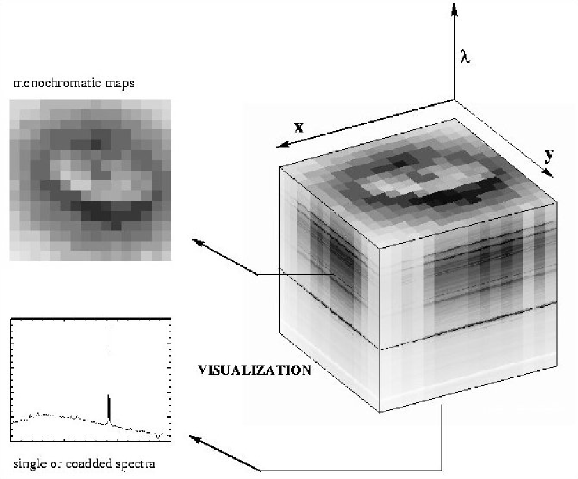
3D spectroscopy, contrary to conventional slit spectroscopy, produces datacubes with full 2-dimensional spatial information within the FOV of the instrument. Fig. 2 shows an idealized datacube with a square field of view, square spatial elements (“spaxels”) along coordinates (x,y), and spectra arranged in columns ( $\lambda$ ). From this entity, one can retrieve monochromatic maps at certain wavelengths (datacube slices), or co-added maps equivalent to broad- or narrow-band images, and single spectra (columns), as well as co-added spectra for any desired region, i.e. digital aperture within the FOV. We stress that with proper spatial sampling, it is possible to record intensity profiles of monochromatic maps. For point sources, this is equivalent to measuring the wavelength-dependent PSF of the target. Conversely, one can use a priori knowledge of the stellar PSF to fit this profile in any datacube slice at the predicted centroid position, and derive a flux estimate even in the presence of a complex and spatially variable background surface brightness distribution.

Considering the observational problems outlined in § 2, and comparing with spectrographs posessing slits of any geometry, we note that there is a number of advantages, which become important especially for background-limited spectroscopy of faint objects :

(1) 3D spectroscopy is insensitive to pointing and guiding errors when observing point sources. XPN at the distance of M31 have equivalent V magnitudes fainter than 21. Near the nucleus, they are normally invisible for broad-band TV acquisition cameras on 4m-class telescopes. With 3D, the slit losses outlined in § 2.1.1 are no longer of concern.

(2) Since there is no fixed physical aperture, an optimal digital aperture can be chosen throughout the datacube, thus optimizing the S/N at any given wavelength and solving the problem of § 2.1.2.

(3) In a datacube, differential atmospheric refraction is observed as a translation in (x,y) as a function of $\lambda$ (Arribas et al. 1998a). Provided that the point source is not located too close to the edge of the field in the direction of translation, it will always be contained in the FOV and available for analysis, solving problem § 2.1.3.

(4) A most serious drawback of slit spectroscopy is the fact that there are only two regions along the slit next to the source, which can be used to estimate the background at the location of the target, setting e.g. the detection limit for Ly_α emitters at 8-10m class telescopes to a few 10^-17 erg/cm²/sec (Morris et al. 2002). This limit is dictated by systematic errors of slit geometry and other instrumental effects, even when the spatial distribution of the night sky background can be assumed to be constant (Glazebrook & Bland-Hawthorne 2001). The situation for the observation of our XPN is considerably worse: the surface brightness of unresolved stars near the nucleus of M31 is up to 7 mag brighter than the continuum of the night sky background, and spatially variable on different scales. Because of the composition of the underlying stellar population, the spatially variable surface brightness distribution may exhibit a variance in absorption line profiles depending on the contribution from stars of different spectral types. In addition, there is a spatially uncorrelated pattern of emission line spectra emerging from H II regions, supernova remnants, the diffuse ISM, and other nebulosities (see Fig. 1).

Contrary to slit spectroscopy, 3D provides the full 2-dimensional spatial information at any wavelength in the vicinity of the target. We will show that fitting a PSF to the XPN image at any wavelength slice of the datacube allows us to provide the best possible discrimination of the point source against the variable background, thus reducing systematic errors which are otherwise unavoidable for slit of fiber spectrographs. The details of this procedure are explained in § 6.

3 Instrumentation

3D instruments have been developed on the basis of different principles: fiber bundles (e.g. Barden & Wade 1988), micro-pupil lens arrays (e.g. Bacon et al. 1995), micro-pupil lens arrays coupled to fibers (e.g. Allington-Smith et al. 1998b), and slicers (e.g. Weitzel et al. 1996). PMAS is based on the fiber-coupled lens array design (see details below). In order to prepare for the use of PMAS already during its construction phase, and for reasons of data reduction software development, a preliminary observing programme was conducted with two other existing 3D instruments.

3.1 MPFS

MPFS¹¹1http://www.sao.ru/{̃}gafan/devices/mpfs/mpfs_main.htm is a 3D instrument featuring the lens array – fiber bundle design. It has been in operation since 1997 in the prime focus of the 6m BTA in Selentchuk, Russia (Si’lchenko & Afanasiev 2000). It has a 16 $\times$ 16 element lens array of square lenses, with a spatial sampling of 0.5 arcsec, 0.75 arcsec, and 1 arcsec at different magnifications, respectively. The 256 spectra are imaged onto a thinned 1K $\times$ 1K SITe TK1024 CCD using a f/1.2 Schmidt-Cassegrain camera. The total efficiency (excluding the atmosphere) is about 5% at 500 nm, dropping steeply towards the blue. From a variety of gratings, dispersions of 1.35 $\ldots$ 5 Å/pixel can be selected.

3.2 INTEGRAL

INTEGRAL²²2http://www.ing.iac.es/{̃}bgarcia/integral/html/integral_home.html is a fiber bundle type of 3D spectrograph at the 4.2m WHT, La Palma (Arribas et al. 1998b). One of three different bundles with 0.45 arcsec, 0.9 arcsec, and 2.7 arcsec projected fiber diameters and with 205, 219, and 135 fibers, respectively, are available to accomodate different observational requirements in terms of spatial resolution and FOV. The fibers are packed in a hexagonal arrangement, filling a rectangular field. The fiber bundles are coupled to WYFFOS, the bench-mounted fiber spectrograph on the Nasmyth platform of the WHT. The detector is a thinned 1K $\times$ 1K CCD at the internal focus of the spectrograph Schmidt camera. Different gratings with dispersions between 0.35 and 6.2 Å/pixel can be used.

3.3 PMAS

PMAS³³3http://www.aip.de/groups/opti/pmas/OptI_pmas.html is a dedicated 3D instrument with a lens array of 16 $\times$ 16 square elements in the present configuration, coupled by means of a fiber bundle to a fully refractive fiber spectrograph, which is currently equipped with a 2K $\times$ 4K thinned CCD (SITe ST002A), providing 2048 spectral bins. A 2 $\times$ 2K $\times$ 4K mosaic CCD, which was commissioned recently, increases the free spectral range to 4096 spectral bins. Along the spatial direction on the CCD, the current setup provides more than twice the space which would be required for the total of 256 fiber spectra. The present fiber bundle has been conservatively manufactured with 100 $\mu$ m diameter, high OH^- doped fibers for good UV transmission. A future upgrade with 50-60 $\mu$ m diameter fibers will replace the existing IFU with a 32 $\times$ 32 element array. The optical system is based on UV-transparent media and provides good transmission in the blue. A unique feature of PMAS is the internal A&G camera, equipped with a LN₂-cooled, blue-sensitive SITe TK1024 CCD, giving images with a scale of 0.2 arcsec/pixel and a FOV of 3.4 $\times$ 3.4 arcmin². The camera can be used with broad-band and narrow-band filters of the standard Calar Alto filter inventory. For a more detailed description, see Roth et al. 2000a and Kelz et al. 2003.

4 Observations

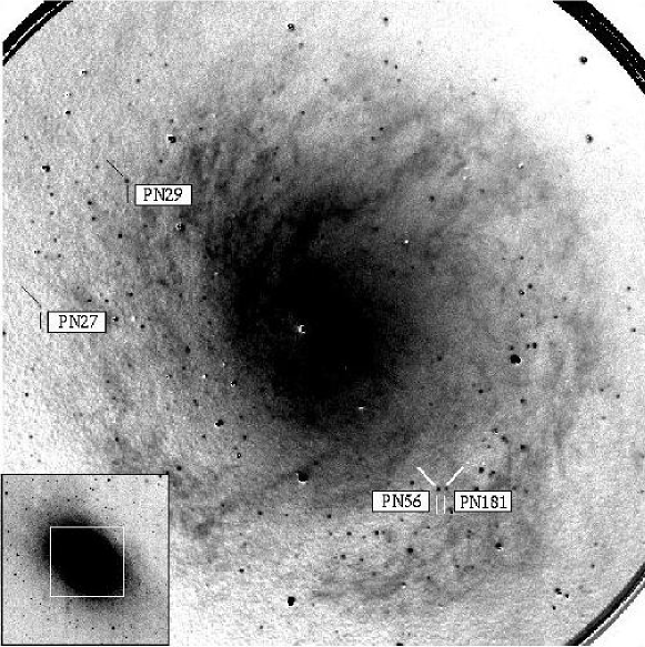
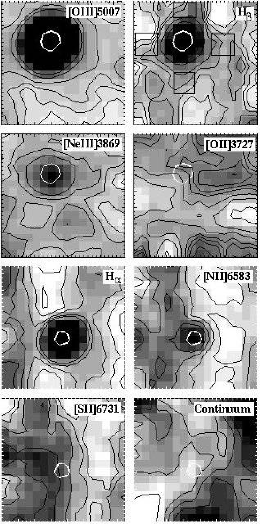
In order to understand the problems of real 3D data and for the purpose of developing the P3d data reduction software (Becker 2002) well before the commissioning of PMAS, we conducted a preliminary programme of observations with other existing instruments (MPFS, INTEGRAL). We selected our targets from the list of CJFN89, supplemented with narrow-band H_α images for the purpose of finding objects which appeared to be critical in terms of background subtraction. The H_α frames were kindly made available to us prior to publication by T. Soffner, University of Munich. The images were taken on September 10, 1994, with the Calar Alto 3.5m prime focus CCD camera, equipped with a Fabry-Perót etalon. The etalon has a passband of $\approx$ 9 Å FWHM and can be scanned in wavelength, thus providing flux and radial velocity information at the same time (Meisenheimer & Hippelein 1992). An example of 3 coadded frames (exposure time 3 $\times$ 1000sec) for a 6 arcmin diameter FOV, centered on the nucleus, is shown in Fig. 1. From the on-band image, a corresponding off-band image has been subtracted, revealing the emission line component with the XPN as point sources, residuals of less than perfectly subtracted stars, and the prominent spiral-like appearance of the ISM emission near the nucleus and throughout the bulge of M31. This feature has been known for some time (Münch 1960). The first optical images were obtained by Jacoby et al. (1985). Spectra by Ciardullo et al. (1988) reveal emission in H_α and the strong low excitation lines of [N II] $\lambda$ $\lambda$ 6548,6583 and [S II] $\lambda$ $\lambda$ 6717,6731, which are responsible for some of the background subtraction problems reported by RC99. This fact is illustrated further with the thumbnail images of our targets in Fig. 3, where the fuzzy and filamentary structure of the emission line background becomes quite obvious.

A log of our observations quoting the different instruments used is given in Table 1. Note that 3D spectra were taken with different wavelength coverage, spectral resolution, and spatial sampling, depending on the instrument and prevailing observing conditions. The object ID numbers were adopted from CJFN89. Each target observation was accompanied by standard star observations and bias, continuum and spectral line lamp calibration frames, which, for best accuracy, where normally taken before and after a series of target exposures at any pointing for MPFS and PMAS, in order to minimize flexure effects. INTEGRAL, employing the bench mounted WYFFOS spectrograph, is insensitive to flexure.

Table 1: Log of Observations.

Date	Instrument	Object	Exposure	Seeing	Grating	$\Delta\lambda$ [Å]	Å/pixel	Flux Standard(s)
06-Nov-1997	MPFS	PN29	3 $\times$ 1200	1.5	V600	4000-6750	2.65	BD+284211, Feige 24
06-Nov-1997	MPFS	PN276	2 $\times$ 900	1.5	V600	4000-6750	2.65	Hiltner-600
18-Sep-1998	MPFS	PN276	2 $\times$ 1200	1.1	V600	4270-6910	2.6	BD+284211, Feige 24
21-Sep-1998	MPFS	PN29	8 $\times$ 1200	1.5-2.0	V600	4210-6850	2.6	Feige 24
27-Sep-1998	MPFS	PN27	4 $\times$ 1800	2.0-2.5	V600	4210-6850	2.6	BD+284211
28-Sep-1998	MPFS	PN27	4 $\times$ 1800	2.5-3.0	V600	4210-6850	2.6	BD+284211
26-Dec-1998	INTEGRAL	PN276	3 $\times$ 1800	1.5	R600B	3540-6660	3.01	SP0305+261, G191-B2B
23-Oct-2001	PMAS	PN276	3 $\times$ 1200	1.5	V600	3550-5200	1.6	HR718
24-Oct-2001	PMAS	PN29	9 $\times$ 1200	1.1	V600	5600-7200	1.6	HR153, HR1544
26-Oct-2001	PMAS	PN29	8 $\times$ 1800	1.4	V600	3550-5200	1.6	HR153, HR1544
31-Aug-2002	PMAS	PN56	4 $\times$ 1800	1.0	U600	3440-5100	1.6	HD192281
01-Sep-2002	PMAS	PN56	9 $\times$ 1200	1.1	U600	3440-5100	1.6	HD192281, HD19445
01-Sep-2002	PMAS	PN181	5 $\times$ 1200	1.1	U600	3440-5100	1.6	HD192281, HD19445

5 Data Reduction

The data reduction for all observations, except for MPFS data of 1997, was performed using the P3d package of Becker (2002). P3d is an IDL code which was originally developed for PMAS, but has been adapted to 3D data from other instruments (SPIRAL, INTEGRAL). The 1997 data were reduced by JS using a modified version of the dofiber task of IRAF ⁴⁴4IRAF is distributed by the National Optical Astronomy Observatories, which is operated by the Association of Universities for Research in Astronomy, Inc. (AURA) under cooperative agreement with the National Science Foundation.. This task involved a considerable amount of interactive work and required to control each of the $\approx$ 256 spectra individually for any single CCD frame, whereas the P3d programme works automatically once a set of parameters has been set appropriately. The various steps of the data reduction procedure are as follows. The raw CCD frames are first bias subtracted and cleaned from cosmic ray events. As an option, P3d allows to apply a correction for pixel-to-pixel CCD response non-uniformity, known as the standard flatfield correction for direct imaging applications. This correction is performed using grossly defocussed continuum flatfield exposures and corrects only for small scale pixel-to-pixel variations. Note that for 3D fiber spectroscopy, there are different levels of response calibration: (1) detector pixel non-uniformity, (2) total spaxel-to-spaxel throughput variation (caused by lens array defects and diffraction, variation in fiber transmission and coupling), and (3) the wavelength-dependent non-uniformity of spaxel-to-spaxel response, which is also linked to the wavelength-dependent variation of the detector QE.

After these first basic procedures, a critical step consisted in the tracing of spectra which became difficult when there was little flux, and thus confusion for automatic procedures, in particular near the edge of a spectral range when the response was dropping steeply. This is where the dofiber routine normally required to correct interactively for misidentifications and errors. P3d includes a geometrical model based on calibration exposures which is cross-correlated and matched with the observed set of spectra for any single exposure in order to avoid this complication. For the case of PMAS, Fig. 4 in Roth et al. 2002b shows how these spectra are arranged on the detector, with comfortably wide inter-order gaps (14 pixels distance), which is an unusual arrangement compared to most other 3D instruments. In order to make efficient use of detector estate, one would normally try to squeeze as many spectra as possible onto the CCD. The inevitable overlap of adjacent spectra to a degree which depends on the distance of spectra and optical quality of the spectrograph optics leads to “crosstalk” with effects as discussed by Roth et al. 2000b, Becker et al. 2000, and investigated in detail by Becker (2002); but see also Allington-Smith & Content 1998. We shall further discuss this issue below.

P3d allows for two different modes of extraction, which is the next step in the data reduction process. The standard mode is to define an extraction swath along the traces and integrate the contained flux for any spectral bin. This is the procedure which is also employed in a subset of P3d routines, forming the PMAS online data reduction software for use at the telescope. Swath extraction fails badly when the spacing of spectra is very dense, in particular for applications where one is interested in faint spectral signatures on a bright background. Such features are likely to be completely wiped out in the presence of crosstalk. This difficult situation was encountered with our MPFS data sets. In order to correct for crosstalk, P3d provides a profile-fitting mode which can be applied when a model for the cross-dispersion profile can be constructed. The details of this procedure are described in a separate paper (Becker, in preparation). Profile-fitting also allows to correct for scattered light, which has been a considerable complication for our MPFS spectra in the blue (Fig. 4 in Roth et al. 2000b).

After extraction, a wavelength calibration is applied using spectral line lamp exposures. This is another step where MPFS with dofiber required human interaction and correction for errors. P3d uses calibration lamp template spectra resulting in a robust procedure with no need for interactive corrections.

The set of extracted and wavelength calibrated spectra was then corrected for spaxel-to-spaxel (or fiber-to-fiber) variations by normalizing to a continuum flatfield exposure. A final correction of the smooth wavelength-dependent spaxel-to-spaxel response variation of order 3-5% rms over the entire wavelength range was provided by means of a twilight sky flatfield exposure for the MPFS (1998) and PMAS frames (“fiber flat”), omitting any disturbing atmospheric features. Using standard star exposures, the set of spectra was then weighted with the instrumental and atmospheric sensitivity function to produce the final flux-calibrated datacube.

The resulting dataset consists of a 2-dimensional frame of stacked spectra which we found to be a convenient arrangement for inspection with a visualisation tool. An example for the appearance of this tool, which allows one to plot maps, single or coadded spectra for mouse-selected digital apertures, is shown in Roth et al. 2002c. The data was finally written to disk in a FITS compatible format whose specification was developed by the Euro3D consortium (Walsh & Roth 2002).

6 Data Analysis and Results

This section is organized as follows: in §§ 6.1 – 6.3 we discuss general properties of our reduced 3D data, the procedure of merging single exposures into a final datacube, our techniques of background subtraction, 3D spectrophotometry, and the final steps to derive the flux-calibrated and dereddened XPN spectra. In §§ 7.1 – 7.5 we present the results for individual objects. If not indicated otherwise, the software used for the various steps was developed under IDL and written by TB.

6.1 3D Point Spread Function

A crucial test as to whether or not the proposed PSF fitting technique would be useful for 3D data consisted in the analysis of standard star datacubes, which were well-enough exposed to provide good S/N in any quasi-monochromatic slice (Fig. 4, upper right plot). The slices were treated like normal, albeit tiny, CCD images, and a Moffat function was fitted independently to the frame of each wavelength bin. As an instructive example, the result for a particularily poor exposure of the standard star HR1544 is shown in Fig. 4, chosen for the purpose of demonstrating that it is indeed possible to determine an accurate and well-defined PSF. The datacube was obtained with the P3d_online data reduction routine without profile fitting. In the two panels in the middle we plot the resulting FWHM fit values in X and Y vs. wavelength, and in the bottom panels the corresponding centroid offsets in X and Y with respect to a wavelength in the middle of the free spectral range. A map of the mean residual of the PSF-fit is displayed in the upper left panel.

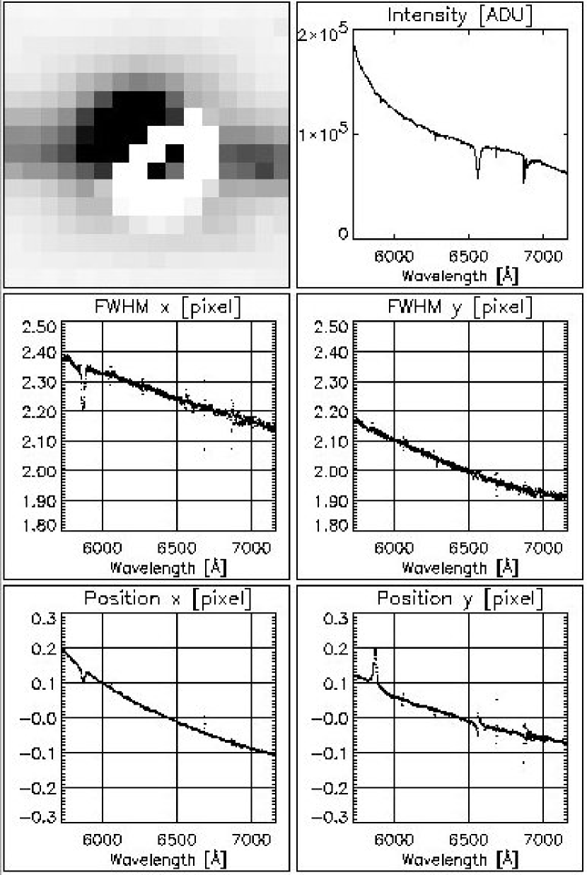
First of all, we note that the centroid is not located at a fixed position, but moves monotonically with wavelength in X and Y. The standard star was observed at an hour angle of 1^h 04^m and at airmass 1.177, with an expected offset due to differential atmospheric refraction of 0.18 arcsec between the wavelengths of 5700 Å and 7300 Å, according to Filippenko (1982). The ambient parameters used for this estimate are a temperature of 9.5^∘C, a relative humidity of 33%, and an atmospheric pressure of 789.8 mbar. The same offset of 0.18 arcsec is obtained in our datacube when we add the X and Y offsets in quadrature (a spatial element corresponding to 0.5 arcsec).

Secondly, it is seen that the scatter about a mean curve is very low: a best fit low order polynomial yields an rms scatter of 0.0015 and 0.0018 spaxels in X and Y, respectively, indicating that the PSF is an extremely sensitive measure of position ( $\pm$ 0.001 arcsec). The obvious flaw near 5800 Å, introducing a systematic error of $\leq$ 0.1 arcsec over a small wavelength interval, is entirely due to a local detector blemish which could not be flatfielded out. The flaw vanishes completely in exposures where the star is centered on another region of the IFU. Likewise, we show that similar systematic errors at a few isolated wavelength bins near the cores of the H_α and other absorption lines are caused by small differential wavelength calibration errors between different sets of spectra and the effects of spectral rebinning.

Thirdly, we observe that the PSF is non-symmetric as seen in the residual image and FWHM plots, indicating an elliptical elongation, and an extended horizontal feature at a level of 1 % peak intensity. This result is instructive in two ways: (a) the horizontal feature illustrates the effect of crosstalk, introduced because of the presence of the extended wings of the fiber spectrograph PSF. The effect amounts to typically 0.5% peak intensity and vanishes when the profile-fitting extraction is applied; (b) the elongation indicates an optical aberration of the 3.5m Telescope, which was in fact identified as decentering coma and astigmatism due to a misalignment of the primary mirror, and which was corrected during a maintenance period shortly after our August 2002 run (Thiele 2003).

Finally, we note that the expected decrease of seeing disk size with wavelength is clearly seen in the plots of FWHM (Fried 1966).

6.2 Co-adding Datacubes, Atmospheric Refraction

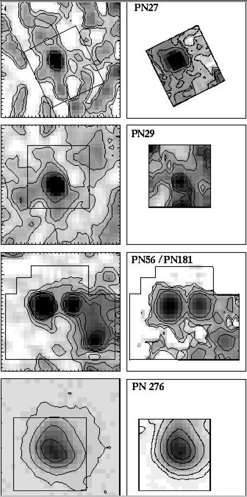
The measurement of faint line intensities of XPN at the distance of M31 using a 4m-class telescope requires total exposure times of order several hours. The combination of datacubes taken over such a period of time is complicated by the fact that each exposure is affected by a different amount of differential atmospheric refraction, i.e. shift of monochromatic slices with wavelength. To counteract this effect, we shifted the slices at the wavelength of interest to a common reference system, which was compensated for refraction, using the formulae of Filippenko (1982). Moreover, the effect of a different amount of atmospheric extinction as a function of airmass had to be taken into account when coadding all datasets to form the final datacube. The set of PMAS exposures taken in October 2001 was suffering from flexure of the telescope guiding camera, which required yet another adjustment. The net effect of flexure, which was confirmed independently with two different daytime tests at the telescope, resulted in an overall shift of order 0.5-1 arcsec per hour, thus requiring to shift these datacubes to compensate both for differential refraction and flexure. Note that this problem has disappeared after commissioning of the PMAS A&G camera, which is internal to the instrument and replaces the telecope TV-Guider system. The necessity to correct for the shifts, however, was an interesting exercise for 3D mosaic exposures of areas larger than provided by the FOV of the IFU. The maps shown in Fig. 3 therefore cover a larger area than normally obtained from the instrumental FOV alone.

We note in passing, that the continuous offsets between the exposures resemble the familiar dithering technique for direct imaging, with the potential advantage of improving the sampling of the PSF, and reducing residual errors of the spaxel-to-spaxel non-uniformity correction (Wisotzki et al. 2003).

6.3 3D Spectrophotometry

The last step to create the spectra of our targets consisted in measuring the flux within a digital aperture or using a PSF fit around the centroid of the fully corrected, final datacube at all wavelengths.

In order to do this accurately enough, one has to subtract a two-dimensional model of the background surface brightness distribution, since contrary to the night sky emission, this light is anything but constant over the field-of-view. In our case, the background consists of the two dominant components: stellar continuum, and diffuse/filamentary ISM emission. As discussed in more detail in § 7, the latter component presented a peculiar problem, since it is difficult to distinguish from the continuum, being responsible for intensity overestimates of some weak XPN emission lines in conventional spectrophotometry.

A two-step procedure was devised to accomplish the modelling and subsequent removal of these components. The XPN case (as opposed to stars) is quite favourable, in that the object continuum (typically 10 ${}^{-3}\times$ I ${}_{H_{\beta}}$ /Å) is completely negligible in comparison with the background intensity of the galaxy . The entire datacube consists essentially of background light, except for the few wavelengths with appreciable XPN emission line flux. Using a normalization scheme for all of the monochromatic slices to take out the continuum spectral features, it was possible to (1) create continuum maps as a function of wavelength, (2) enhance the contrast of the ISM emission line filaments, and (3) create a map of the emission component. The background correction was finally completed by subtracting the two components from the original datacube. The technical details of this procedure are described in Becker (2002).

Although we cannot completely rule out the possibility that at the wavelengths of strong background absorption or emission line features the chance alignment of PSF-compatible anomalies with the XPN, i.e. unrelated point sources, would remain undetected and cause systematic errors of the XPN line fluxes, we expect that the probability of such chance alignments is small. In general we find that our continuum subtraction yields flat spectra which are free of obvious residuals (Fig. 5), contrary to the examples discussed in § 2.1.

Because of the relatively high contrast of the [O III] $\lambda$ 5007 line in an almost featureless region of the background continuum, the centroid was defined to an accuracy of a fraction of a spaxel (e.g. 0.1 arcsec in the case of PN29), and the flux was obtained directly from aperture photometry. Using a standard star curve-of-growth analysis, an aperture correction was applied to account for the flux lost outside of the digital aperture. The PSF at this wavelength was determined as a 2-dimensional gaussian and used as a template for the other, fainter emission lines with a correction for the wavelength-dependent variation of the seeing FWHM. Since the measurements are background shot-noise dominated, a more sophisticated PSF characterization was unnecessary.

The final procedure was then to fit the wavelength-dependent model PSF to each datacube slice, constrained by the centroid of the bright [O III] feature. Note that the fit allows for negative fluxes, which, in the presence of noise, avoids a positive bias of the detection probability. Note also that the absence of any limiting apertures (slit effects) justifies the term spectrophotometry.

6.4 2-Channel Deconvolution

As a more sophisticated method to separate a point source from the background, we used the two-channel Richardson-Lucy deconvolution algorithm cplucy (Lucy 1994) which is available within IRAF. It is optimized for improved photometric performance and avoids the artifacts and oscillations that are known for the standard RL-Algorithm (Hook & Lucy 1993). The two-channel method makes use of the precise knowledge of the location of one or several point sources, and iterates the point source channel separately from another channel, which is processing the smoothly varying background. We applied the algorithm to our datacubes such that each monochromatic slice was subject to an independent cplucy run. The PSF is defined by one of the bright lines, e.g. [O III] $\lambda$ 5007, corrected for the weakly varying FWHM as a function of wavelength as determined from standard star exposures. The flux of the point source detection in each slice in the end created the final spectrum. Details of the application of the two-channel deconvolution method to the peculiar case of a datacube, the treatment of a photometric bias in the case of very low background intensity levels, and various tests are described in more detail in Becker (2002).

As a drawback, we note that the procedure of fitting an optimized PSF to the centroid of an XPN in each wavelength bin (i.e. monochromatic map), is forced to produce detections with flux $\geq 0$ . The resulting spectra have non-normal noise distributions. They were preferrentially used for confusion-limited cases and to determine upper limits for faint, background-limited lines.

6.5 Dereddened Line Intensities

The emission line intensities were measured after flux-calibrating the extracted XPN spectra with standard star exposures by fitting gaussians at the nominal wavelengths, corrected for the radial velocity shift known from the bright [O III] line. This step was performed within the ESO-MIDAS data reduction package and through use of a line fitting tool kindly provided by A. Schwope (AIP). We have assessed the statistical errors of these fits by implanting artificial emission lines with known intensities at several (typically $\approx$ 100) different wavelengths near the original line into the data, fitting these simulated lines, and evaluating the standard error of a single measurement from the variance of the whole set. The dereddening based on the Balmer decrement followed the standard procedure as described by RC99.

The final results for our objects are listed in Tab. 2. The errors for typical line intensities (faint/intermediate/bright lines) are listed as S/N values at the end of the table.

Table 2: REDDENING-CORRECTED LINE STRENGTHS.

$\lambda$ [Å]	Ion	PN27	PN29	PN29	PN56	PN181	PN276	PN276	PN276
		MPFS	MPFS	PMAS	PMAS	PMAS	MPFS	INT.	PMAS
3727	[O II]	…	…	¡26	¡38	¡83	…	…	820
3869	[Ne III]	…	…	145	26	95	…	84	71
3889	He I, H I	…	…	¡15	¡29	¡74	…	…	29
3969	[Ne III], H I	…	…	56	¡26	¡71	…	32	40
4101	H_δ	…	…	40	17	¡67	…	…	31
4340	H_γ	47	48	43	46	¡64	49	51	47
4363	[O III]	37	…	19	27	¡64	19	29	12
4686	He II	…	23	19	¡19	¡62	…	…	11
4861	H_β	100	100	100	100	100	100	100	100
4959	[O III]	542	612	565	399	368	117	122	118
5007	[O III]	1645	2030	1698	1282	1121	365	376	345
5755	[N II]	…	…	¡5	…	…	10	10	…
5876	He I	17	12	12	…	…	11	12	…
6300	[O I]	…	…	10	…	…	69	83	…
6360	[O I]	…	…	¡5	…	…	24	26	…
6548	[N II]	…	16	15	…	…	124	157	…
6563	H_α	286	286	286	…	…	304	310	…
6583	[N II]	13	48	35	…	…	380	381	…
6678	He I	…	…	15	…	…	…	…	…
6717	[S II]	…	18	¡5	…	…	193	180	…
6731	[S II]	…	30	¡5	…	…	188	176	…
7065	He I	…	…	¡5	…	…	…	…	…
7135	[Ar III]	…	…	12	…	…	…	…	…
	Uncertainties	(in %):
4363	[O III]	…	…	14.3	9.4	…	…	…	19.6
4861	H_β	…	9.1	3.3	2.5	6.6	…	…	2.3
5007	[O III]	…	0.7	0.6	0.4	0.8	…	…	0.7
m₅₀₀₇		20.81	20.95	21.01	20.96:	21.88:	19.99:	20.13:	20.45
c		0.34	0.41	0.30	0.33	0.33	…	…	…

7 Discussion

7.1 PN29

This is the best-studied object of our sample. It was observed in 3 different observing runs with the MPFS and PMAS instruments. We had selected PN29 initially for the 1997 MPFS run because of its relatively high brightness among the CJFN89 XPN (m₅₀₀₇ = 21.01), being located nevertheless close enough to the nucleus of M31 to study the systematic effects of different background subtraction techniques (132 arcsec north-east from nucleus). Coincidently, PN29 is one of the objects in common of the JC99 and RS99 samples, where the two sets of measurements produced conflicting results, which can now be reconciled with our new 3D observations. JC99 give a detailed account of their measurement and the difficulties to match the observed line intensities with a physically reasonable photoionization model. The data presented two major problems: firstly, their [O III] $\lambda$ 5007/H_β line ratio of 14.8 is significantly different from the value of 22.2 reported by RS99. The discrepancy is completely incompatible with the respective error estimates, so that the difference remained a mystery. Secondly, the [S II] line ratio I( $\lambda$ 6717)/I( $\lambda$ 6731) with a value of 1.76 is at the low-density limit, which required to invoke a two-zone ionization model in order to match the observed line intensities. Since, as a result, the sulfur abundance of this model was unusually high ([S/H]=+0.5), the authors considered the possibility of an artifact due to the weakness of the sulfur lines and the difficult background subtraction.

Concerning the first problem, an example of our new data is shown in Fig. 8. The spectrum was obtained from the combined datacube of a total of four 1800sec exposures using a 600 lpmm grating (1.65 Å/pixel) by co-adding 4 spectra within a square digital aperture of 1 $\times$ 1 arcsec². Next to [O III] $\lambda$ 5007 and $\lambda$ 4959, H_β is seen in emission on the blue wing of the stellar background absorption line. The thick line is the spectrum of the background alone, derived as the average from an annulus of 50 spaxels of radius=3 arcsec around the central aperture and scaled to a best match of the target spectrum. Due to the large number of contributing spectra, the background spectrum has very little noise. Although at first glance the agreement with the continuum of the XPN aperture appears to be satisfactory, a closer inspection reveals that a measurement of the XPN H_β line intensity is sensitively depending on the details of the background definition. Obviously, in order to arrive at an accurate line intensity estimate, it is necessary to properly account for the slope of the absorption line profile in the process of background subtraction.

We have simulated the background subtraction of conventional slit spectroscopy by coadding flux in virtual horizontal and vertical slitlets adjacent to the point source, as indicated by the rectangles in the H_β map of Fig. 7. Linear interpolation within each slitlet pair yields the spectra shown in the lower left panel of Fig. 8 (thin full line: horizontal, dash-dotted line: vertical slit). By way of inspecting the continuum map (Fig. 7), the offset between the two curves is readily explained: the vertical slitlet pair is sampling, on average, a somewhat brighter background surface brightness than the horizontal slit does, while the XPN centroid is located near a local minimum of the continuum background surface brightness distribution. Therefore, the slit-based values are overestimating the background at the location of the point source, which is probably also why the JC99 continuum spectrum of PN29 exhibits an overall negative offset from zero. An attempt to bring the two former curves into agreement by scaling them to a best match with the source spectrum outside of the H_β feature, however, fails in the core of the absorption profile: the vertical slit predicts a significantly shallower absorption than the horizontal slit does (lower right panel in Fig. 8). The difference can be made plausible by realizing that the background is increased by a diffuse emission component, which partially fills in the absorption profile (H_β map in Fig, 7) – a familiar problem known also from integrated light population studies (cf. remarks in § 1). In our exercise, the horizontal slitlet pair is less effected by the ISM filament than the vertical one, thus producing the deeper absorption trough. Numerically, the difference translates into [O III] $\lambda$ 5007/H_β line ratios of 12.0 and 19.5, respectively.

Although it is unlikely that our simulation is capable of reproducing exactly the measurements of JC99 and RS99, respectively, we can offer a sensible explanation for the discrepancy between their H_β results: most likely the difference was caused by a different setup of the slit orientation. From this experiment it becomes clear that the simple slit approach is insufficient to provide an accurate background model as required for a reliable determination of the contaminated XPN H_β line intensity. In contrast, the result of our PSF fitting procedure with cplucy is plotted as the thick line in the bottom panels of Fig. 8, the dashed line indicating the background channel alone. The [O III] $\lambda$ 5007/H_β line ratio from this analysis is 17.0. An important consequence of the smaller H_β intensity compared to JC99 is an increase of our value for the logarithmic extinction from c = 0.14 to c = 0.30.

Concerning the problem of the [S II] doublet $\lambda$ $\lambda$ 6717,6731, which appeared to be unusually bright (I( $\lambda$ 6717)=51) in the data of JC99, these lines are not even detected in our spectrum. They must be significantly fainter than this value, with a conservative upper limit of I( $\lambda$ 6717) $\leq$ 5. A closer inspection of the [S II] map in Fig. 7 shows that the XPN is embedded in a fuzzy structure of background emission, which most probably has caused the overestimate suspected by JC99. We note in particular that at the location of the PSF centroid determined from H_α, no local maximum is visible in [S II]. Furthermore, our map in [O II] $\lambda\lambda$ 3727,3729 also does not reveal a trace of any local maximum, contrary to the nearby [Ne III] $\lambda$ 3869, which is well-defined. The 5 $\sigma$ upper limit for [O II] is I( $\lambda\lambda$ 3727,3729) $\leq$ 26.

These findings do not come entirely as a surprise. The ISM spectra of M31 presented by Ciardullo et al. 1989 show strong emission in the low excitation lines of [S II] $\lambda$ $\lambda$ 6717,6731 and [N II] $\lambda$ $\lambda$ 6548,6583, with line strengths comparable to H_α. After careful modelling and subtraction of the continuum, we have produced a flux-calibrated spectrum of the gaseous emission background component (Fig. 9), which compares well with the result of Ciardullo et al. 1989. Note that the order of magnitude of the [S II] $\lambda$ 6717 flux within a 2” slit is compatible with the PN29 line intensity of 4 $\times 10^{-16}$ erg/cm²/sec measured by JC99, which the authors had suspected to be affected by background contamination. We also confirm that the discrepant [S II] $\lambda$ $\lambda$ 6717,6731 line ratio of 1.76 is due to the background filament, and not intrinsic to PN29.

In order to highlight the sensitivity to background contamination, we have plotted the JC99 and RSM99 line intensities vs. our PMAS results, normalized to I( $\lambda$ 5007Å)=100 (Fig. 10). First of all, there is general agreement with JC99 for the high excitation and Balmer lines within the error bars, except for [Ne III] $\lambda$ 3967, which we measure a factor of 0.8 fainter. Since our spectrum is somewhat noisier due to a shorter total exposure time (4 hours as compared to 6.5) and probably a higher blue atmospheric extinction at the site (Hopp & Fernandez 2002), we cannot rule out an error. We note, however, that RSM99 quote a value even lower than ours (0.6 $\times$ JC99), so that we do not consider the difference to be significant. More importantly, there is a striking disagreement for the low excitation lines [O II] $\lambda$ 3727, [N II] $\lambda$ $\lambda$ 6548,6583, and [S II] $\lambda$ $\lambda$ 6717,6731, for all of which we derive significantly lower values (or upper limits, respectively). We thus confirm that indeed the suspected background contamination is present not only for [S II], but also for other ions, including [O II].

7.2 PN27

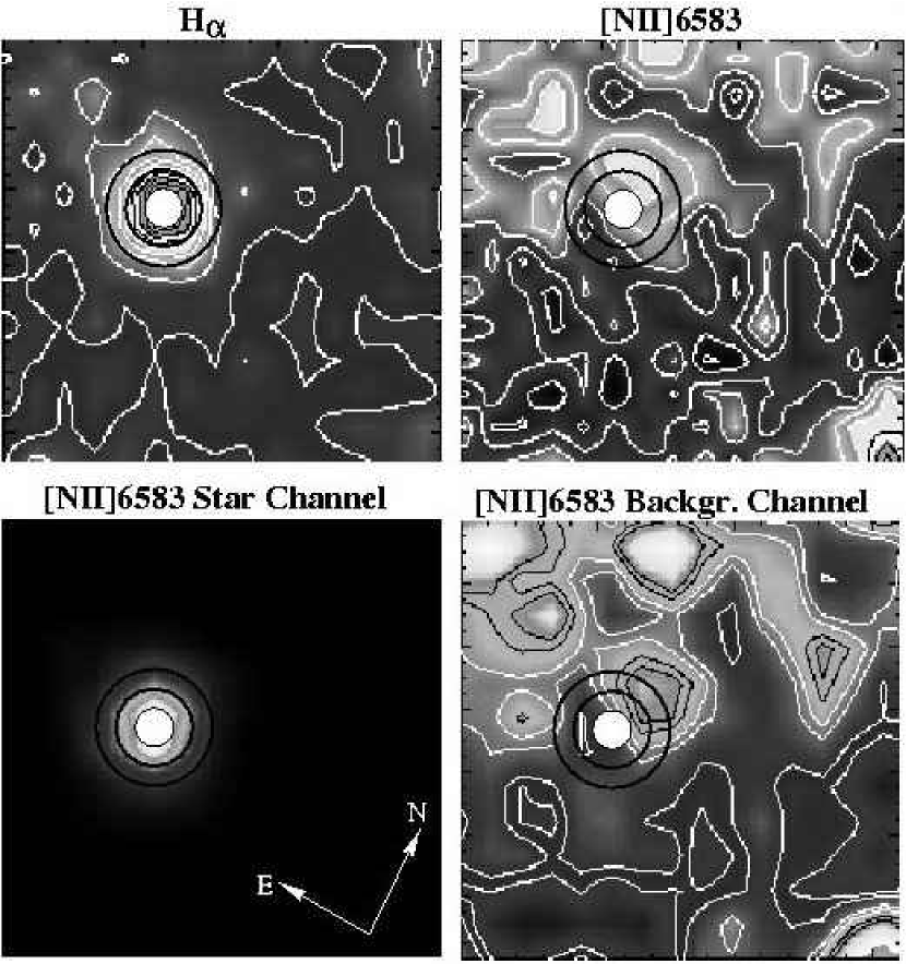
This object is located 152” east of the nucleus and is among the brightest of the CJFN89 survey (m₅₀₀₇ = 20.85). JC99 were able to obtain an excellent spectrum, allowing them to construct one of the best-constrained models of their XPN sample. A large number of well-determined emission lines, in particular the presence of a bright [O III] $\lambda$ 4363, provided sufficient confidence in the resulting model fit. Nevertheless, JC99 note the general faintness of the low ionization lines like [N II] and [S II], the latter of which are just marginally present, giving an indication of a line ratio close to the low density limit. Our MPFS spectrum, resulting from 8 exposures with a total exposure time of 4 hours under mediocre seeing conditions (2”-3”), is consistent with JC99 as far as the brighter lines are concerned (Tab. 2). For the fainter lines such as [S II] $\lambda$ 6717,6731, the S/N is not sufficient to draw any firm conclusions. Nevertheless, the measurable [N II] $\lambda$ 6583 line presented us with a very good opportunity to apply the cplucy deconvolution technique, which uses our a priori knowledge of the location and shape of the PSF as a criterion for the separation of the point source flux from the background. At the wavelength of this emission line, the map shows again a background emission filament which is partially overlapping with the contours of the point source as derived from the bright nearby H_α line (Fig. 11, upper panels). We applied the cplucy algorithm to investigate in how far the filamentary intensity is affecting a conventional measurement of the point source emission at the locus of PN27, and in how far it is possible to separate the two components. The lower panels of Fig. 11 show separate [N II] $\lambda$ 6583 maps for the point source and the background channel, respectively, after processing with cplucy. The ISM filament, which is also seen in the direct FP image in Fig. 3, is very bright in proportion to the XPN, and, owing to its vicinity to the centroid of the point source, practically impossible to detect with the very limited spatial resolution of a slit. Even our datacube aperture spectrophotometry using a background annulus resulted in an overestimate of the XPN emission in this line: 3.1 $\times 10^{-16}$ erg/cm²/sec. The upper limit derived with cplucy amounts to (1.2 $\pm 0.3)$ $\times 10^{-16}$ erg/cm²/sec . This result is only half the line strength reported by JC99 and RSM99. The important conclusion from this experiment is, that slit spectroscopy is indeed critically subject to systematic errors in crowded field environments, and that 3D provides a good tool to overcome these limitations, as one would have expected from the long-standing experience with crowded field CCD photometry. As for the particular target PN27, a more accurate measurement of [N II] $\lambda$ 6583 and other faint emission lines would clearly benefit from an 8-10m class telescope with superior image quality, e.g. the GMOS-IFU at the Gemini-North telescope (Allington-Smith et al. 2000).

7.3 PN56

PN56 is another test case with suspected low-ionisation background contamination, but bright enough in [O III] to provide a well-defined PSF ( m₅₀₀₇ = 20.94 ). The XPN is located 120 arcsec south-west of the nucleus. The suspicious filament extends in an arc-like distribution to the West/South-West, also affecting another nearby object (PN181) which is observed simulataneously in the same FOV (Fig. 3). A third surface brightness maximum in H_α is seen about 9 arcsec SW of PN56. The somewhat irregular outline of the map in Fig. 3 is the result of dithering, allowing us to cover a larger FOV than provided by the IFU alone. The observations were performed with PMAS during comissioning of the U600 grating. Due to poor weather conditions (clouds), only spectra in the blue were recorded. The spectrum of PN56 (Fig. 5) exhibits a relatively bright H_β of I([O III] $\lambda$ 5007)/I( $\lambda$ 4861)=12.8, and the lines of H_γ, H_δ, [O III] $\lambda$ 4363, and [Ne III] $\lambda$ 3869. For other lines like He II $\lambda$ 4686, [O II] $\lambda$ 3727,3729, [Ne III] $\lambda$ 3968 we were merely able to derive upper limits.

7.4 PN181

PN181 is located 4.5 arcsec west of PN56. It is the faintest of our objects, with m₅₀₀₇ = 21.85. It is embedded in an environment with significant filamentary emission. Since the target was included merely in a fraction of the exposures contributing to the mosaic with PN56, the total integration time is only 6000 sec. The quality of the exposure was also affected by poor transmission of the atmosphere and clouds. The spectrum is dominated by photon shot noise of the background such that only [O III] $\lambda$ $\lambda$ 5007,4959, H_β and [Ne III] $\lambda$ 3968 are detected with confidence (Fig. 5). At the 2 $\sigma$ -level, there are hints of H_γ and H_δ, but we refrain from further analysis at this unsufficient level of signal-to-noise.

7.5 PN276

Spectra of this object were secured for the first time by JS during the 1997 MPFS run at the 6m BTA (Schmoll 2001). PN276 had been selected after a series of non-detections of other targets due to pointing problems, since it is a relatively bright object (m₅₀₀₇ = 20.48), which was expected to be more easily recognized on the raw CCD frame. It is also located further out in the disk (r_nucl=820 arcsec) and therefore less subject to background subtraction problems. We remind the reader that despite the aforementioned advantage of 3D with regard to pointing accuracy, direct target acquisition using a standard broadband TV guiding camera is extremely difficult, if not impossible, because of the lack of contrast, thus demanding blind offset pointing (cf. Fig. 2 in Roth et al. 2002b). PN276 was also considered interesting because of the opportunity of observing simultaneously two objects within the same FOV (PN276, PN277 in Ford & Jacoby 1978, of which the latter, however, was no longer listed in CJFN89). Already from the inspection of monochromatic maps which were produced by the MPFS online data reduction software, a suspicious extended, triangular shape of the object became obvious. Considering the spatial extension, and the spectrum with untypically bright low excitation lines (e.g. [O I] $\lambda$ 6300), it became quickly clear that this object could not be explained as a single XPN, or the superposition of two XPNe with small angular separation. As an interesting comparative test case, PN276 was subsequently reobserved also with MPFS in 1998, with INTEGRAL in 1998, and with PMAS in 2002. The resulting flux-calibrated spectra are shown in Fig. 6. While the 1998 observations with MPFS and INTEGRAL were obtained with similar spectral resolution and wavelength coverage, the PMAS observations were chosen to extend further into the blue at twice the dispersion. Although this spectrum becomes increasingly noisy towards the atmospheric cutoff, the extraordinary strength of [O II] I( $\lambda$ 3727,3729)=820 is clearly visible. The fitted line intensities for each observation are listed in Tab. 2, showing good agreement between the different instruments.

In an attempt to understand the physical nature of this object, the XPN hypothesis can clearly be ruled out. Firstly, the [S II] doublet $\lambda$ 6717,6731 line ratio of 1.03 implies an electron density of $\approx$ 400 e^-/cm³, which is low for a typical PN. Secondly, T ${}_{e}\approx 55000$ K, derived from the [O III] line ratio (I( $\lambda$ 4959) + I( $\lambda$ 5007)) / I( $\lambda$ 4363) is too high. Thirdly, the spatial extension of approximately 5” $\times$ 4” is incompatibel with the typical angular size of an XPN at a distance of 770 kpc (¡ 0.1”). For an H II region, again, the electron temperature is too high. The spectrum matches very well the general signature of supernova remnants (SNR) as explained e.g. in Osterbrock (1989): strong [S II] $\lambda$ 6717,6731, [O II] $\lambda$ 3727,3729, and [O I] $\lambda$ 6300,6364 all of which are indicative of shock-excitation rather than photoionization. The high value of T_e is typical for SNR, as well as the low electron density. With log(I(H_α)/I([N II])) = -0.22 vs. log(I(H_α)/I([S II])) = -0.1 in the diagnostic diagram of Sabbadin & D’Odorico (1976), PN276 is located unambiguously in the SNR region, far away from H II regions or PNe. The projected size of 15 $\times$ 12 pc², confirmed with our direct CAFOS images in [O III] $\lambda$ 5007 and H_α (Fig. 3) is also only plausible for a SNR. Finally, the coincidence with an X-ray source at the same position, detected in the ROSAT PSPC survey of M31 (Supper 1997) and flagged as possible SNR (ID249) provides further evidence that PN276 is in fact a SNR: the position of 0 42 16.93 +41 18 41.5 (1975) as listed in CJFN89 differs by only 2.7” of the ROSAT position of 0 42 16.9 +41 18 38.8, precessed from 2000 to 1975, in accord with the PSPC error circle of 5 arcsec and the astrometric accuracy of $\approx$ 1 arcsec quoted in CJFN89.

8 Summary and Conclusions

Our pilot study has demonstrated the usefulness of integral field (3D) spectroscopy for spectrophotometry of faint planetary nebulae in M31. We have observed 5 objects, two of which (PN27, PN29) could be compared with previously published data. Of the three new spectra, one reveals that the object (PN276) had been misclassified as an XPN. Spatial extension, characteristic properties of the spectrum and positional coincidence with a previously detected X-ray source indicate with a high level of confidence that the source is a SNR.

Thanks to the full 2-dimensional spatial information of the observing technique, we make explicitely use of the a priori knowledge of the PSF, which is conveniently determined from the bright XPN [O III] $\lambda$ 5007 emission line. The PSF is used as a constraint to disentangle the point source flux from contaminating contributions that are due to diffuse or filamentary gaseous emission in the bulge of M31. We find that the low excitation XPN line intensities [O II] I( $\lambda$ 3727,3729), [N II] $\lambda$ 6548,6583, and [S II] $\lambda$ $\lambda$ 6717,6731 tend to be overestimated in previous measurements with classical spectrographs. We have measured the emission line intensity of the ISM component and find that the fluxes corresponding to a typical spectrograph aperture are compatible with a level of background contamination required to explain the systematic discrepancies in line intensities, which have been reported in the literature. Simulated slit spectroscopy from a datacube for PN29 allowed us to produce arbitrary line ratios for I([O III] 5007Å)/I(H_β), suggesting an explanation for the discrepancy reported by JC99 and RSM99. We have employed successfully the cplucy deconvolution algorithm to achieve the best separation of point sources from a highly complex background, both in terms of spectral and of spatial variation.

A fundamental conclusion is that the limited geometry of conventional slit spectroscopy is ill-suited to solve the problem of background subtraction of faint sources embedded in complex, high surface brightness crowded fields. Our results support and quantify the previously suspected notion that such measurements suffer significantly from systematic errors. 3D spectroscopy offers the unique opportunity to make full use of the 2-dimensional spatial and 1-dimensional spectral information of a datacube to construct the best possible background model and eliminate these problems. At the other extreme, single fiber multi-object spectroscopy in high surface brightness regions is obviously a very limited technique and most vulnerable to systematic errors since there is no practical way to provide reliable background estimates in the immediate vicinity of the point source (but see Durrell et al. 2003 for excellent results from a radial velocity survey based on [O III] of XPN in M51). It must be stressed, however, that 3D does not necessarily provide dramatic improvements in S/N for photon-starved observations, but rather allows one to eliminate the systematic errors discussed in this paper.

As a side-remark, we note that, in contrast to the conclusions of Allington-Smith & Content (1998a), residual cross-talk between adjacent spectra on the CCD is potentially dangerous for PSF-fitting algorithms, since the net effect is a distortion of the PSF (cf. Fig. 4), which must be expected to vary with FOV, wavelength, and time. Analogous to the reasoning of Mateo (1998) concerned with CCD photometry, the distortion is not important for the fitting of faint stars, however very much so for applications requiring a good definition of the PSF (cf. Wisotzki et al. 2003).

In continuation of our successful pilot study, we are pursuing a guaranteed observing time programme targeting XPN in M31 and other local group galaxies. The analysis of our present and the expected new data by comparison with ionization models following the receipe described by JC99 will be published in a forthcoming paper.

We have begun to use 3D spectrophotometry for a number of other applications which benefit from the evaluation of spatial information and the PSF, e.g. spectrophotometry of SN2002er (Christensen et al. 2003; see also Aldering et al. 2003 for a description of the SNAP experiment), the quadruple lensed QSO HE 0435-1223 (Wisotzki et al. 2003), optical counterparts of superluminous X-ray sources (Lehmann et al., in prep.), LBV candidates in M33 (Fabrika et al., in prep.). Although our XPN study was facilitated by the availability of the bright emission in [O III] $\lambda$ 5007Å, which is a rather fortunate case to determine a well-defined PSF, we stress that the PSF fitting technique, in particular when using the two-channel cplucy algorithm in combination with high-resolution HST images, opens a new window for solving the difficult observational problems of resolved stellar populations in nearby galaxies.

Although an upgrade of the present IFU with a 32 $\times$ 32 element lens array is underway, increasing the diameter of the FOV by a factor of 2, the multiplex advantage of PMAS for the rather sparsely distributed XPNe in nearby galaxies is very limited. This fact is a direct consequence of the baseline design, which favours wavelength coverage over the maximum number of spectra in terms of detector space, making PMAS a rather unique instrument. Normally, PMAS can observe only one target at a time. With a typical rate of one object per night, the efficiency may appear prohibitively low. On the other hand, we note that in a recent paper by Magrini et al. (2003), out of 42 XPN candidates in M33, observed during 2 nights with the WYFFOS multi-object fiber spectrograph at WHT, only 3 spectra of were found to be of sufficient quality for an abundance analysis.

Clearly, the spectrophotometry of our XPN targets would benefit substantially from the light-collecting power and image quality of a modern 8-10m class telescope, pushing the source confusion problem to fainter limits and providing better S/N for the weak lines which are so crucial for the plasmadiagnostic analysis ([O III] $\lambda$ 4363, [S II] $\lambda$ 6717,6731, etc.). Multi-object spectroscopy of supergiant stars has already been demonstrated to be feasible out to distances beyond the local group with reasonable integration times on the order of $\approx$ 10 hours (Bresolin et al. 2001). The single-target approach of our pilot study would be unrealistically expensive. However, the use of a multi-object deployable IFU instrument in combination with the techniques described in this paper would eventually become an extremely powerful tool for crowded-field spectroscopy and the study of resolved stellar populations in local galaxies, one of the key science cases of the proposed new generation of Extremely Large Telescopes with diameters of 30-100m. As a promising alternative strategy, complex 3D instruments with arcmin FOV and of order 10⁵-10⁶ spatial elements are currently under investigation for the 2nd Generation Instrumentation Plan at the ESO-VLT (Bacon et al. 2002, Morris et al. 2002).

Part of this work was supported by the German Deutsche Forschungsgemeinschaft, DFG under grant HA1850/10-3 , and by the German Verbundforschung des BMBF, grant 05AL9BA1. The authors would like to thank Till Soffner, University of Munich, and Hans Hippelein, MPIA Heidelberg, for providing us with the H_α Fabry-Pérot image of M31 . MMR, TB and JS are indebted to Victor Afanasiev and Seguei Dodonov, Special Astrophysical Observatory in Selentchuk, Russia, for their hospitality and help with MPFS observations at the 6m BTA, for an introduction into 3D data reduction, and for fruitful discussions and insight into integral field spectroscopy. We are thankful to Evencio Mediavilla for generously providing us with INTEGRAL observing time. JS would like to thank Evencio Mediavilla and Stefano Ciroi for introducing him into IFU data reduction techniques under IRAF. The excellent support of Calar Alto staff during the PMAS commissing phase and in operation is gratefully acknowledged.

References

Aldering et al. (2002) Aldering, G. et al. 2002, Proc. SPIE, 4835, 146
Allington-Smith & Content (1998a) Allington-Smith, J., Content, R. 1998a, PASP110, 1216
Allington-Smith, Content, & Haynes (1998b) Allington-Smith, J. R., Content, R., & Haynes, R. 1998b, Proc. SPIE, 3355, 196
Allington-Smith et al. (2000) Allington-Smith, J. R., Content, R., Dodsworth, G. N., Murray, G. J., Ren, D., Robertson, D. J., Turner, J. E., & Webster, J. 2000, Proc. SPIE, 4008, 1172
Arnaboldi et al. (2002) Arnaboldi, M. et al. 2002, AJ, 123, 760
Arribas et al. (1998a) Arribas, S., Mediavilla, E., Garcia-Lorenzo, B., del Burgo, C., Fuensalida, J.J. 1998a, A&AS136, 189
Arribas et al. (1998b) Arribas, S., Cavaller, L., Garcia-Lorenzo, B., Garcia-Marin, A., Herreros, J.M., Mediavilla, E., Pi, M., del Burgo, C., Fuentes, J., Rasilla, J.L., Sosa, N. 1998b, in Fiber Optics in Astronomy III, eds. S. Arribas, E. Mediavilla, F. Watson, ASP Conf. Ser. Vol.152, p. 149
Avila et al. (1997) Avila, G., Rupprecht, G., Beckers, J.M. 1997, Proc. SPIE Vol. 2871, p.1135
Bacon et al. (1995) Bacon, R., Adam, G., Baranne, A., Courtes, G., Dubet, D., Dubois, J. P., Emsellem, E., Ferruit, P., Georgelin, Y., Monnet, G., Pecontal, E., Rousset, A., Say, F. 1995, A&AS, 113, 347
Bacon et al. (2002) Bacon, R., et al. 2002, in Scientific Drivers for ESO Future VLT/VLTI Instrumentation, eds. J. Bergeron, G. Monnet, Springer, Berlin, p. 108
Barden & Wade (1988) Barden, S. C. & Wade, R. A. 1988, ASP Conf. Ser. 3: Fiber Optics in Astronomy, 113
Becker et al. (2000) Becker, T., Roth, M.M., Schmoll, J. 2000, Proc. Imaging the Universe in Three Dimensions: Astrophysics with Advanced Multi-Wavelength Imaging Devices, ASP Conf. Ser. Vo. 195, eds. W. van Breugel, J. Bland-Hawthorn, p.544
Becker (2002) Becker, T. 2002, Thesis, University of Potsdam
Boulesteix (2002) Boulesteix, J. 2002, in it Galaxies: The Third Dimension, ASP Conf. Proc., Vol. 282, eds. Margarita Rosado, Luc Binette, and Lorena Arias, p.374
Bregman, Hogg, & Roberts (1992) Bregman, J. N., Hogg, D. E., & Roberts, M. S. 1992, ApJ, 387, 484
Bresolin et al. (2001) Bresolin, F., Kudritzki, R. P., Méndez, R. H., Przybilla, N. 2001, ApJ548, L159
Chiosi & Carraro (2002) Chiosi, C. & Carraro, G. 2002, MNRAS, 335, 335
Christensen et al. (2003) Christensen, L., Becker, T., Jahnke, K., Kelz, A., Roth, M. M., Sanchez, S. F., Wisotzki, L. 2003, A&A401, 479
(19) Ciardullo, R., Rubin, V. C., Ford, W. K., Jacoby, G. H., Ford, H.C. 1988, AJ95, 438
Ciardullo et al. (1989) Ciardullo, R., Jacoby, G.H., Ford, H.C., Neill, J.D. 1989, ApJ339, 53
Ciardullo (2003) Ciardullo, R. 2003, Workshop on ”Stellar Candles for the Extragalactic Distance Scale”, held in Concepcion, Chile, astro-ph/0301279
de Zeeuw et al. (2002) de Zeeuw, P. T., Bureau, M., Emsellem, E., Bacon, R., Carollo, C. M., Copin, Y., Davies, R. L., Kuntschner, H., Miller, B. W., Monnet, G., Peletier, R. F., Verolme, E. K., 2002, MNRAS, 329, 513
(23) Dopita, M. A., Vassiliadis, E., Wood, P. R., Meatheringham, S. J., Harrington, J. P., Bohlin, R. C., Ford, H. C., Stecher, T. P., Maran, S. P. 1997, ApJ474, 188
Durrell et al. (2003) Durrell, P.R., Mihos, J.C., Feldmeier, J.J., Jacoby, G.H., Ciardullo, R. 2003, ApJ582, 170
Feldmeier et al. (2003) Feldmeier, J. J., Ciardullo, R., Jacoby, G. H., Durrell, P. R. 2003, ApJS145, 65
Filippenko (1982) Filippenko, A. V. 1982, PASP94, 715
Ford & Jacoby (1978) Ford, H., Jacoby, G.H. 1978, ApJS38, 351
Ford et al. (2002) Ford, H., Peng, E., Freeman, K. 2002, in The Dynamics, Structure & History of Galaxies, ASP Conf. Proc. Vol. 273, eds. G.S. Da Costa and H. Jerjen, p.41
Freeman & Bland-Hawthorn (2002) Freeman, K., Bland-Hawthron, J. 2002, Annu. Rev. Astron. Astophys. Vol. 40, p.487
Fried (1966) Fried, D.L. 1966, J.Opt.Soc.Am. 56, 1372
Gerhard, Arnaboldi, Freeman, & Okamura (2002) Gerhard, O., Arnaboldi, M., Freeman, K. C., & Okamura, S. 2002, ApJ, 580, L121
Glazebrook & Bland-Hawthorn (2001) Glazebrook, K. & Bland-Hawthorn, J. 2001, PASP, 113, 197
Goudfrooij, de Jong, Hansen, & Norgaard-Nielsen (1994) Goudfrooij, P., de Jong, T., Hansen, L., & Norgaard-Nielsen, H. U. 1994, MNRAS, 271, 833
Hawarden et al. (2003) Hawarden, T.G., D.Dravins, G.F.Gilmore, R.Gilmozzi, O.Hainaut, K. Kuijken, B.Leibundgut, M.R.Merrifield, D.Queloz, R.F.G.Wyse 2003, Proc. SPIE Vol. 4840, p. 299
Hoessel & Melnick (1980) Hoessel, J. G. & Melnick, J. 1980, A&A, 84, 317
Hook & Lucy (1993) Hook, R.N., Lucy, L.B. 1993, in Proc. Science with the HST, p. 245
Hopp&Fernandez (2001) Hopp, U., Fernandez, M. 2002, Calar Alto Newsletter No.4,
http://www.caha.es/newsletter/news02a/boletin4.html
Hui (1995) Hui, X., Ford, H. C., Freeman, K. C., Dopita, M. A. 1995, ApJ449, 592
Jacoby et al. (1985) Jacoby, G. H., Ford, H., Ciardullo, R. 1985, ApJ290, 136
(40) Jacoby, G. H., Kaler, J. B. 1993, ApJ417, 209
Jacoby & Ciardullo (1999) Jacoby, G. H., Ciardullo, R. 1999, ApJ515, 169
Kelz, Roth, & Becker (2003) Kelz, A., Roth, M. M., & Becker, T. 2003, Proc. SPIE, 4841, 1057
Kudritzki (1998) Kudritzki R.P. 1998, in Stellar Astrophysics for the Local Group. A first step to the Universe - 8th Canary Island Winter School, eds. A. Aparicio, A. Herrero, F. Sanchez, New York, Cambridge Univ. Press., p. 149
Larson (1974) Larson, R. B. 1974, MNRAS166, 585
Lucy (1994) Lucy, L.B. 1994, in The Restoration of HST Images and Spectra II, eds. R. Hanisch & R. White, p. 79
Madore & Freedman (1991) Madore, B.F., Freedman, W. 1991, PASP103, 933
Magrini et al. (2003) Magrini, L., Perinotto, M., Corradi, R. L. M., Mampaso, A. 2003, A&A400, 511
Mateo (1998) Mateo, M. 1998, in Stellar Astrophysics for the Local Group. A first step to the Universe - 8th Canary Island Winter School, eds. A. Aparicio, A. Herrero, F. Sanchez, New York, Cambridge Univ. Press., p. 407
Mehlert et al. (2000) Mehlert, D., Saglia, R. P., Bender, R. Wegner, G. 2000, A&AS141, 449
Meisenheimer & Hippelein (1992) Meisenheimer, K. & Hippelein, H. 1992, A&AS264, 455
Méndez et al. (2001) Méndez, R. H., Riffeser, A., Kudritzki, R.-P., Matthias, M., Freeman, K. C., Arnaboldi, M., Capaccioli, M., & Gerhard, O. E. 2001, ApJ, 563, 135
Meza, Navarro, Steinmetz, & Eke (2003) Meza, A., Navarro, J. F., Steinmetz, M., & Eke, V. R. 2003, ApJ, 590, 619
Monteverde et al. (1997) Monteverde, M. I., Herrero, A., Lennon, D. J., Kudritzki, R.-P. 1997, ApJ474, L107
Morris (2002) Morris, S., Content, R., Sharples, R., Bower, R., Davies, R., Baugh, Carlton 2002, in Scientific Drivers for ESO Future VLT/VLTI Instrumentation, eds. J. Bergeron, G. Monnet, Springer, Berlin, p. 99
Münch (1960) Münch, G. 1960, AJ, 65, 55
Najita & Strom (2002) Najita, J. & Strom, S. E. 2002, Proc. SPIE, 4835, 1
Osterbrock (1989) Osterbrock, D.E. 1989, Astrophysics of Gaseous Nebulae and Active Galactic Nuclei, University Science Books, Mill Valley
(58) Richer, M. G., Stasińska, G., McCall, M. L. 1999, A&AS135, 203
Roth, Seydack, Bauer, & Laux (1997) Roth, M. M., Seydack, M., Bauer, S., & Laux, U. 1997, Proc. SPIE, 2871, 1235
Roth et al. (2000) Roth, M. M. et al. 2000a, Proc. SPIE, 4008, 277
Roth, Becker, & Schmoll (2000) Roth, M. M., Becker, T., & Schmoll, J. 2000b, ASP Conf. Ser. 195: Imaging the Universe in Three Dimensions, 122
(62) Roth, M.M., Becker, T., Böhm, P., Kelz, A. 2002a, Proc. Scientific Drivers for ESO Future VLT/VLTI Instrumentation, eds. J. Bergeron, G. Monnet, Springer, p. 136
Roth, Becker, & Kelz (2002) Roth, M. M., Becker, T., & Kelz, A. 2002b, ASP Conf. Ser. 282: Galaxies: the Third Dimension, 403
Roth, Becker, Böhm, & Kelz (2002) Roth, M. M., Becker, T., Böhm, P., & Kelz, A. 2002c, ASP Conf. Ser. 282: Galaxies: the Third Dimension, 411
Sabbadin & D’Odorico (1976) Sabbadin, F., D’Odorico, S. 1976, A&A49, 119
(66) Saglia, R. P., Maraston, C., Greggio, L., Bender, R., Ziegler, B. 2000, A&A360, 911
Sarazin & Tokovinin (2002) Sarazin, M. & Tokovinin, A. 2002, in Proc. Beyond conventional adaptive optics, eds. E. Vernet, R. Ragazzoni, S. Esposito, and N. Hubin, ESO Conference and Workshop Proceedings, Vol. 58, p. 321
Schmoll (2001) Schmoll, J. 2001, Thesis, University of Potsdam
(69) Shaver, P. A., McGee, R. X., Netwon, L. M., Danks, A. C., Pottasch, S. R. 1983, MNRAS204, 53
Si’lchenko&Afanasiev (2000) Si’lchenko, O., Afanasiev, V. 2000, A&A364, 479
Smartt et al. (2001) Smartt, S. J., Crowther, P. A., Dufton, P. L., Lennon, D. J., Kudritzki, R. P., Herrero, A., McCarthy, J. K., Bresolin, F. 2001, MNRAS325, 257
Supper et a. (1997) Supper, R., Hasinger, G., Pietsch, W., Trümper, J., Jain, A., Magnier, E.A., Lewin, W.H.G., v. Paradijs, J. 1997, A&A317, 328
Thiele, U. (2003) Thiele, U. 2003, Calar Alto Newsletter No.5,
http://www.caha.es/thiele/Newsletter/align35.html
Urbaneja et al. (2003) Urbaneja, M.A., Herrero, A., Bresolin, F., Kudritzki, R.-P., Gieren, W., Puls, J. 2003, ApJ584, L73
Venn et al. (2000) Venn, K., McCarthy, J.K., Lennon, D.J., Pryzbilla, N., Kudritzki, Lemke, M. 2000, ApJ541, 610
Venn et al. (2001) Venn, K. A., Lennon, D. J., Kaufer, A., McCarthy, J. K., Pryzbilla, N., Kudritzki, R. P., Lemke, M., Skillman, E. D., Smartt, S. J. 2001, ApJ547, 765
(77) Walsh, J. R., Walton, N.A., Jacoby, G. H., Peletier, R.F. 1999, A&A346, 753
(78) Walsh, J.R., Jacoby, G.H., Peletier, R.F., Walton, N.A. 2000, Proc. SPIE Vol. 4005, p.131
Walsh & Roth (2002) Walsh, J. R. & Roth, M. M. 2002, The Messenger, 109, 54
Weitzel et al. (1996) Weitzel, L., Krabbe, A., Kroker, H., Thatte, N., Tacconi-Garman, L. E., Cameron, M., & Genzel, R. 1996, A&AS, 119, 531
(81) White, S.D.M. 1980, MNRAS191, 1
(82) Wisotzki, L., Becker, T., Christensen, L., Helms, A., Jahnke, K., Kelz, A., Roth, M.M., Sanchez, S.F. 2003, astro-ph/0307147
(83) Worthey, G., in Chemical Evolution from Zero to High Redshift, eds. J. R. Walsh, M. R. Rosa, Springer, Heidelberg, p. 168
Wyse et al. (2000) Wyse, R.F.G., Olsen, K., Rich, M., O’Connell, R. 2000, in The GSMT Book: Report of the Stellar Populations Panel,
http://www.aura-nio.noao.edu/book/index.html
Zaritsky, Kennicutt, & Huchra (1994) Zaritsky, D., Kennicutt, R. C., & Huchra, J. P. 1994, ApJ, 420, 87