Fragmentation and the formation of primordial protostars: the possible role of Collision Induced Emission

Abstract

The mechanisms which could lead to chemo-thermal instabilities and fragmentation during the formation of primordial protostars are investigated analytically. We introduce new analytic approximations for H₂ cooling rates bridging the optically thin and thick regimes. These allow us to discuss chemo–thermal instabilities up to densities when protostars become optically thick to continuum radiation ($n\equiv\rho/m_{H}\lower 2.15277pt\hbox{$\;\buildrel<\over{\sim}\;$}10^{16-17}\;{\rm cm^{-3}}$). During the proto-stellar collapse instabilities are active in two different density regimes. In the well known “low density” regime ($n\sim 10^{8}-10^{10}\;{\rm cm^{-3}}$), instability is due to 3-body reactions quickly converting atomic hydrogen into H₂. In the “high density” regime ($n\lower 2.15277pt\hbox{$\;\buildrel>\over{\sim}\;$}10^{14}\;{\rm cm^{-3}}$), another instability is triggered by the strong increase in the cooling rate due to H₂ Collisional Induced Emission (CIE). In agreement with the three dimensional simulations, we find that the “low density” instabilities cannot lead to fragmentation, both because fluctuations are too small to survive turbulent mixing, and because their growth times are too slow. The situation for the newly found “high density” instability is analytically similar. This continuum cooling instability is as weak as “low density” instability, with similar ratios of growth and dynamical time scales, as well as allowing for the necessary fragmentation condition $t_{cool}\lower 2.15277pt\hbox{$\;\buildrel<\over{\sim}\;$}t_{dyn}$. Because the instability growth timescale is always longer than the free fall timescale, it seems unlikely that fragmentation could occur in this high density regime. Consequently, one expects the first stars to be very massive, not to form binaries nor harbour planets. Nevertheless, full three dimensional simulations are required to be certain. Such 3D calculations could become possible using simplified approaches to approximate the effects of radiative transfer, which we show to work very well in 1D calculations, giving virtually indistinguishable results from calculations employing full line transfer. This indicates that the effects of radiative transfer during the initial stages of formation of primordial proto–stars are local corrections to cooling rather than influencing the energetics of distant regions of the flow.

1 Introduction

In current scenarios for the formation of the first stars, molecular hydrogen plays a prominent role, providing the only cooling mechanism for metal-free gas at $T\lower 2.15277pt\hbox{$\;\buildrel<\over{\sim}\;$}10^{4}\;{\rm K}$. H₂ cooling is responsible for both the collapse of the gas inside the small ($M_{\rm halo}\sim 10^{6}\;M_{\odot}$) cosmological halos where primordial star formation is believed to occur (e.g. Couchman & Rees 1986; Tegmark et al. 1997, Abel et al. 1998), and for the fragmentation of the gas itself into “clumps” with masses of $\sim 100-1000\;M_{\odot}$, as is seen in the simulations of Abel, Bryan & Norman (1998, 2000) (see also Bromm, Coppi & Larson 2002). The fate of these objects is unclear. Several previous studies, based on analytical arguments (i.e. stability analysis) or single-zone models, led to different conclusions about the fragmentation properties of primordial clouds. One important instability-triggering mechanism was first suggested by Palla, Salpeter & Stahler (1983; hereafter PSS83): the onset of 3-body H₂ formation at number densities $n\lower 2.15277pt\hbox{$\;\buildrel>\over{\sim}\;$}10^{8}\;{\rm cm^{-3}}$ (where $n\equiv\rho/m_{\rm H}$) causes a fast increase in the cooling rate, possibly leading to fragmentation on a mass scale of $\sim 0.1M_{\odot}$. A similar result was obtained by Silk (1983; hereafter S83) by applying a criterion for “chemo-thermal instability” (first discussed by Sabano & Yoshii, 1977) to an object where 3-body H₂ formation is important.

Numerical simulations have recently shed new light upon the issue, and in particular Abel, Bryan & Norman (2002; hereafter ABN02) were able to reach the 3-body reactions density regime finding that these reactions actually lead to the formation of a single fully molecular core (with a mass of $\sim 1\;M_{\odot}$) at the centre of each clump. They point out that in their simulations they see several chemo-thermally unstable regions, but that the instabilities do not lead to fragmentation because turbulence efficiently mixes the gas, erasing each fluctuation before it can grow significantly. Recently, Omukai & Yoshii (2003; OY03) found a somewhat different explanation by improving the original S83 investigation and pointing out that instabilities growth was too slow.

The further evolution of such an object is still uncertain: due to the high molecular fraction, many of the numerous H₂ roto-vibrational lines (accounting for most of the cooling) become optically thick just after the formation of the molecular core. For this reason, it becomes impossible to estimate the H₂ cooling rate without a complete treatment of radiative transfer, which currently can not be included into full 3-D hydrodynamical simulations. Simpler 1-D studies, such as those in Omukai & Nishi (1998; hereafter ON98) and Ripamonti et al. (2002; hereafter R02), can follow the further evolution, giving useful predictions about the physical processes driving the collapse, or about the properties of the small hydrostatic protostellar core which finally forms in the centre; on the other hand, their intrinsic spherical symmetry prevents them from giving direct predictions about fragmentation.

An interesting result of ON98 and R02 is that during the collapse, the protostellar object experiences a phase when cooling is dominated by the effects of H₂ Collision-Induced Emission (CIE), the opposite process of the more commonly known Collision-Induced Absorption, or CIA. Both of them find that, at the beginning of the CIE-cooling phase, the molecular core is optically thin to CIE-produced continuum photons, and there is a very fast increase in the cooling rate until the continuum optical depth exceeds unity. However, neither of these previous studies pointed out that during this phase the core conditions resemble the ones that, at the onset of 3-body H₂ formation, led to the chemo-thermal instability: the core is optically thin (which is believed to be a necessary condition for fragmentation; see Rees 1976) and the cooling rate is undergoing a dramatic increase.

In the next sections, we will investigate more thoroughly the issue of chemo-thermal instability, with special attention to the effects of CIE cooling. In section 2 we will describe the main cooling processes, giving a brief account of CIE emission, and some useful approximations for H₂ line cooling. In section 3 we examine the conditions for the insurgence of chemo-thermal instabilities, and argue whether they can cause fragmentation. Finally, we discuss the results in section 4.

2 Cooling processes

2.1 Collision-Induced Emission

H₂ molecules have no electric dipole, and emission or absorption of radiation can take place only through quadrupole transitions. But when a collision takes place, the interacting pair (H₂-H₂, H₂-He, H₂-H) briefly acts as a “supermolecule” with a nonzero electric dipole, and an high probability of emitting (CIE) or absorbing (CIA) a photon (see the brief discussion in Lenzuni, Chernoff & Salpeter 1991, or Frommhold 1993 for an extensive account). In the same way, during an H-He collision, the two atoms perturb each other and there is a relevant probability of emission (or absorption) of a photon through a dipole transition. Because of the very short collision times ($\Delta t\lower 2.15277pt\hbox{$\;\buildrel<\over{\sim}\;$}10^{-12}\;{\rm s}$ for $T\lower 2.15277pt\hbox{$\;\buildrel>\over{\sim}\;$}300\;{\rm K}$), collision-induced lines become very broad, actually merging into a continuum; for example, in the H₂ CIE spectrum only the vibrational bands can be discerned as smooth peaks deriving from the merging of the roto-vibrational lines.

2.1.1 CIE cooling rate

Table 1: List of references for the various kind of collisions leading to CIE emission. We also specify the temperature range and the maximum frequency considered.

Pair	T[K]	$\nu_{\rm max}$[cm-1]	Reference
H2-H2	400-1000	17000	Borysow 2002
H2-H2	1000-7000	20000	Borysow et al. 2001
H2-He	1000-7000	20088	Jorgensen et al. 2000
H2-H	1000-2500	10000	Gustafsson, Frommhold 2003
H2-H	400-1000	6000	Gustafsson et al. 2003
H-He	1500-10000	11000	Gustafsson, Frommhold 2001

The shape of CIE spectra can be found in the literature (see Table 1 for a list of references), and used for estimating the cooling rates due to the main CIE processes. The definition of the monochromatic emission coefficient $j_{\nu}$ (cfr. Rybicki & Lightman, eq. 1.15)

$$dE=j_{\nu}\,dV\,d\Omega\,dt\,d\nu$$ (1)

(where $E$ is the energy emitted, and $j_{\nu}$ has units of ${\rm erg\,cm^{-3}\,ster^{-1}\,s^{-1}\,Hz^{-1}}$) can be easily integrated to give the luminosity per unit mass $L$

$$L\equiv{{dE}\over{dt\,dm}}={{dE}\over{dt\,\rho dV}}={{4\pi}\over{\rho}}\int{j_{\nu}d\nu}.$$ (2)

The gas can be assumed to be in thermal equilibrium, so that $j_{\nu}=\alpha_{\nu}B_{\nu}(T)$ (where $B_{\nu}(T)$ is the Planck function at temperature $T$), and the cooling rate per unit mass due to emission induced by collisions between particles of species $i$ and species $j$ in a gas of temperature $T$ and density $\rho$ is

$$L_{i,j}(T,\rho,y_{i},y_{j})={{4\pi}\over{\rho}}\int{\alpha_{\nu,i,j}(T,\rho,y_{i},y_{j})B_{\nu}(T)d\nu},$$ (3)

where $y_{i}$ and $y_{j}$ are the mass fractions of particles of species $i$ and $j$, respectively. We took the values of the collision-induced absorption coefficient $\alpha_{\nu,i,j}$ from the references listed in Table 1.

It can be seen that these references provide a complete set of data only in a relatively narrow temperature range ($1500\;{\rm K}\leq T\leq 2500\;{\rm K}$). By a fortunate coincidence, this is also the temperature range where CIE cooling dominates over all the other cooling mechanisms (see next section), and where CIE effects are more pronounced. However, we have artificially extended this range to the full extension of the H₂-H₂ data range ($400\;{\rm K}\leq T\leq 7000\;{\rm K}$) by estimating the cooling rates $L_{i,j}(T)$ which are not directly available, through the assumption that the ratio $L_{i,j}(T)/L_{\rm H_{2},H_{2}}(T)$ is the same as at the closest known value. This assumption is somewhat arbitrary, but has negligible effects for a gas where H₂ is the dominant species (which is the most relevant case); in the case of a gas with a high atomic fraction, and outside the $1500\;{\rm K}-2500\;{\rm K}$ temperature range, the results shown in Fig. 2 are only indicative.

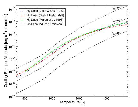
Figure 1: Comparison of H₂ line cooling rate and H₂-H₂ CIE cooling rate. Thick lines denote the line cooling rate as calculated by Galli & Palla 1998 (short dashes), Martin, Schwarz & Mandy 1996 (long dashes) and Lepp & Shull 1983 (dots); these were calculated assuming to be in the high density regime ($n\lower 2.15277pt\hbox{$\;\buildrel>\over{\sim}\;$}10^{8}\;{\rm cm^{-3}}$), where the cooling per molecule is independent of density. Thin solid lines denote CIE cooling rates at molecular number densities $n_{\rm H_{2}}=10^{14}\;{\rm cm^{-3}}$ (bottom line), $n_{\rm H_{2}}=10^{15}\;{\rm cm^{-3}}$ (middle line) and $n_{\rm H_{2}}=10^{16}\;{\rm cm^{-3}}$ (top line). If the considered object were optically thin to H₂ line cooling, CIE would become important at number densities $n\lower 2.15277pt\hbox{$\;\buildrel>\over{\sim}\;$}10^{15}\,{\rm cm^{-3}}$.

In Fig. 1 we compare the CIE cooling rates of a pure H₂ gas at different densities (similar results hold also for H₂-He and H₂-H-He mixtures) with the H₂ line cooling rates calculated by several other authors. CIE cooling overcomes roto-vibrational line cooling at an H₂ number density $n_{\rm H_{2}}$ between $10^{14}$ and $10^{16}\;{\rm cm^{-3}}$, the exact value depending on the gas temperature. This values can change because of the effects of optical depth, and are appropriate only when both CIE cooling and H₂ line cooling occur in an optically thin regime. Instead, both ON98 and R02 (treating CIE by means of the Planck opacities given by Lenzuni et al. 1991) found that H₂ line cooling starts to be limited by optical depth at an early stage, when CIE cooling is still optically thin. As a result, in their models CIE starts to overcome H₂ lines at a relatively low density (corresponding to $T_{c}\simeq 1600\;{\rm K}$, $n_{{\rm H_{2}},c}\simeq 5\times 10^{13}\;{\rm cm^{-3}}$, where the $c$ subscript refers to the conditions in their central regions; see Fig. 4 of R02).

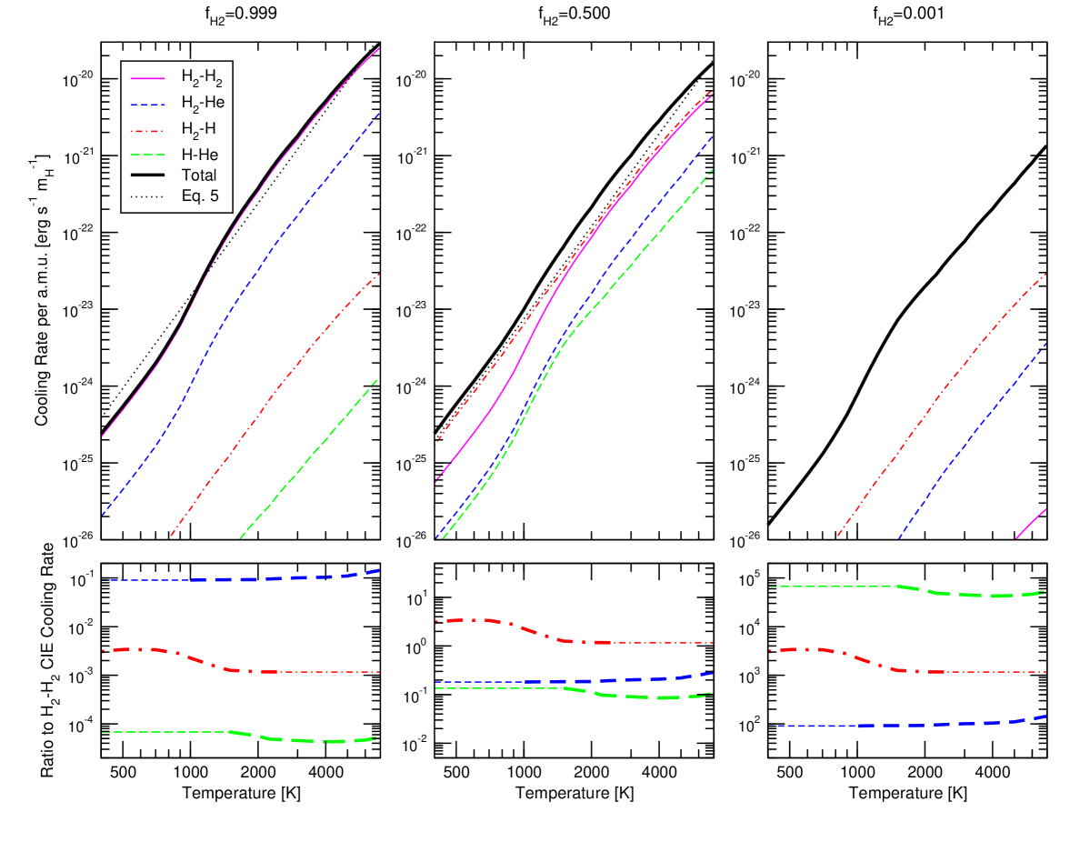
Figure 2: Comparison of CIE cooling rates for different kinds of collisions. Top panels show the cooling rates per unit mass as a function of temperature, for a gas with different molecular fractions ($f_{\rm H_{2}}=0.999$, $0.5$ and $0.001$). The thick solid line denotes the total CIE cooling, the thin lines denote the single components: H₂-H₂ (thin solid), H₂-He (short dashed), H₂-H (dot dashed) and H-He (long dashed); the dotted lines in the upper left and upper center panels show the results of eq. (5). Note that in the top-left panel the total and H₂-H₂ lines are practically indistinguishable, as well as the total and the H-He lines in the top-right panel. The bottom panels show the ratios of the last three components to the CIE cooling rate due to H₂-H₂ collisions; in these panels the line thickness indicates whether the ratio was taken from one of the references in table 1 (thick lines) or it was assumed to be constant at the closest known value (thin lines). All the quantities were calculated assuming $n=10^{14}\;{\rm cm^{-3}}$ and $y_{\rm He}=0.25$.

The gas chemical composition determines which kind of collisions contribute most to total cooling. In Fig. 2 we show the temperature dependency of the cooling rate due to each kind of collisions for three different molecular fractions, $f_{\rm H_{2}}=0.999$, $0.5$ and $0.001$, where $f_{\rm H_{2}}\equiv{{{2n_{\rm H_{2}}}}\over{n_{\rm H}+2n_{\rm H_{2}}}}$ is the mass fraction of H₂ (relative to all the H atoms). The He mass fraction is kept fixed at $y_{\rm He}=0.25$ (the value we will use throughout the rest of this paper), and the assumed density is $\rho=1.67\times 10^{-10}{\rm g\,cm^{-3}}$ (i.e. $n=10^{14}\;{\rm cm^{-3}}$). As can be expected, H₂ collisions (especially H₂-H₂) dominate CIE cooling when hydrogen is mostly molecular, but their importance declines with decreasing H₂ fraction, becoming negligibly small for mostly atomic gas. The total CIE cooling rate for molecular gas is substantially (20-30 times) larger than for atomic gas in the same conditions.

2.1.2 Approximate CIE cooling rate

In the rest of this paper, the only relevant case will be the one with $f_{\rm H_{2}}\simeq 1$. In that case, the total CIE cooling rate (per unit mass)

$$L_{\rm CIE}(\rho,T,y_{\rm H},y_{\rm H_{2}},y_{\rm He})=L_{\rm H_{2},H_{2}}+L_{\rm H_{2},H}+L_{\rm H_{2},He}+L_{\rm H,He}$$ (4)

can be reasonably approximated by a power law

$$L_{\rm CIE}(\rho,T,y_{\rm H},y_{\rm H_{2}},y_{\rm He})\simeq L_{\rm CIE}(\rho,Y,f_{\rm H_{2}})=A_{\rm CIE}\;\rho\,T^{\alpha}\,Xf_{\rm H_{2}}$$ (5)

with $\alpha\simeq 4.0$ and $A_{\rm CIE}\simeq 0.072\;{\rm erg\,cm^{3}\,g^{-2}\,s^{-1}K^{-4.0}}$, and where $X=1-y_{\rm He}=0.75$ is the total hydrogen mass fraction. As can be seen in fig. 2, this approximation holds down to $f_{\rm H_{2}}\sim 0.5$, although very roughly.

2.2 H₂ line cooling

2.2.1 Optically thin H₂ line cooling

At the moderately high densities we are interested in ($n\lower 2.15277pt\hbox{$\;\buildrel>\over{\sim}\;$}10^{6}\;{\rm cm^{-3}}$), the populations of H₂ roto-vibrational levels can be found through the LTE assumption, and the H₂ line cooling is quite well known (see Fig. 1). Here we will use the LTE rate first given by Hollenbach & McKee (1979), which was also used by Galli & Palla (1998) as an high density limit.

$$L_{\rm lines,HM}(\rho,T,f_{\rm H_{2}})={{Xf_{\rm H_{2}}}\over{m_{H}}}{\mathcal{H}}(T_{3}),$$ (6)

where $L_{\rm lines,HM}$ is the H₂ lines cooling rate per unit mass, $T_{3}\equiv{T\over{1000\;{\rm K}}}$, and

$${\mathcal{H}}(T_{3})= \left({{9.5\times 10^{-22}T_{3}^{3.76}}\over{1+0.12T_{3}^{2.1}}}\right)e^{-\left({{0.13}\over{T_{3}}}\right)^{3}}+3\times 10^{-24}e^{-{{0.51}\over{T_{3}}}}+$$ (7)

$$6.7\times 10^{-19}e^{-{{5.86}\over{T_{3}}}}+1.6\times 10^{-18}e^{-{{11.7}\over{T_{3}}}}\quad{\rm erg\,s^{-1}}.$$

Eq. (6) is actually an analytic fit to the sum of the luminosities of all the roto-vibrational lines (which instead was used by ON98 and R02):

$$L_{\rm lines,thin}(T)={{Xf_{\rm H_{2}}}\over{2m_{H}}}\sum_{m,n}{h\nu_{m,n}A_{m,n}\left[{{{2J_{n}+1}\over{U(T)}}e^{{E_{n}}\over{k_{\rm B}T}}}\right]}$$ (8)

where $\nu_{m,n}$ is the frequency of the H₂ transition from level $n$ downward to level $m$, $A_{m,n}$ is the spontaneous radiative decay rate (Einstein coefficient) of the transition, $J_{n}$ is the rotational quantum number associated with level $n$, $E_{n}$ is the energy of level $n$ and $U(T)=\sum_{i}{(2J_{i}+1)e^{E_{i}/(k_{\rm B}T)}}$ is the H₂ partition function at temperature $T$. The sum in (8) is over all H₂ lines, with each term representing the total luminosity of an H₂ molecule in the considered line. We note that the term in square brackets represents the fraction of H₂ molecules in the roto-vibrational level $n$.

2.2.2 Optically thick H₂ line cooling

The above cooling rates (eq. 6 and 8) can only be applied to optically thin objects. In reality, as 3-body reactions start transforming the bulk of hydrogen into molecular form, the core regions of the contracting protostellar clouds quickly become optically thick to H₂ line radiation (ON98, R02). As a result, the effective cooling rate falls well below the one predicted in the optically thin case.

It is possible to find a reasonable approximation to the “effective” cooling rate in the central regions of a collapsing protostellar object. The density profile of such an object can be approximated with a central flat “core” (where also temperature and chemical composition are approximately constant) surrounded by an “envelope” where the density decreases as a power-law ($\rho\propto r^{-2.2}$, according to both ON98 and R02). Such a density profile is predicted by the Larson-Penston self-similar solution (Larson 1969; Penston 1969), which applies fairly well. Another correct prediction that can be inferred from the Larson-Penston solution is that the mass of the central “core” is of the order of the Bonnor-Ebert mass (i.e. the critical mass for gravitational collapse of an isothermal sphere given an external pressure $P_{\rm ext}$; see Ebert 1955 and Bonnor 1956), as calculated using the central value of temperature ($T_{c}$), number density ($n_{c}=\rho_{c}/m_{\rm H}$), molecular weight ($\mu_{c}$) and mean adiabatic index ($\gamma_{c}$)

$$M_{{\rm BE},c}\simeq 20\;{\rm M_{\odot}}\left({T_{c}\over{\rm 1\;K}}\right)^{3/2}\left({n_{c}\over{\rm 1\;cm^{-3}}}\right)^{-1/2}\mu_{c}^{-2}\gamma_{c}^{2};$$ (9)

from this a “Bonnor-Ebert radius” can be estimated

$$R_{{\rm BE},c}=\left({{{3M_{{\rm BE},c}}\over{4\pi n_{c}m_{H}}}}\right)^{1/3}\simeq 1.8\times 10^{19}\;{\rm cm}\;\left({T_{c}\over{\rm 1\;K}}\right)^{1/2}\left({n_{c}\over{\rm 1\;cm^{-3}}}\right)^{-1/2}\mu_{c}^{-2/3}\gamma_{c}^{2/3}.$$ (10)

The H₂ column density from the centre to infinity is then

$$N_{{\rm H_{2}},c} \simeq R_{{\rm BE},c}{{n_{c}Xf_{{\rm H_{2}},c}}\over 2}+\int_{R_{{\rm BE},c}}^{\infty}{{{n_{c}Xf_{\rm H_{2}}(r)}\over 2}\left({r\over{R_{{\rm BE},c}}}\right)^{-2.2}dr}=$$ (11)

$$= R_{{\rm BE},c}{{n_{c}Xf_{{\rm H_{2}},c}}\over 2}\left\{{1+\int_{1}^{\infty}{[f_{\rm H_{2}}(xR_{{\rm BE},c})/f_{{\rm H_{2}},c}]x^{-2.2}dx}}\right\}$$

where $x\equiv r/R_{{\rm BE},c}$. This last equation leads us to define a parameter $\xi$ such that

$$N_{{\rm H_{2}},c}\equiv\xi R_{{\rm BE},c}{{n_{c}Xf_{{\rm H_{2}},c}}\over 2}$$ (12)

and whose approximate value (cfr. eq. 11) is

$$\xi\simeq 1+\int_{1}^{\infty}{[f_{\rm H_{2}}(xR_{{\rm BE},c})/f_{{\rm H_{2}},c}]x^{-2.2}dx}.$$ (13)

Since we are considering objects in which $f_{\rm H_{2}}$ is maximum at the centre, equation (13) implies that $1\leq\xi\leq 1.8$, but in Table 2 (see columns 6 and 7) we show that this is not the case. The main reasons are that the density inside the core actually decreases from the centre outward, and that the Bonnor-Ebert mass provides an estimate of the core size which is not very accurate (Table 2, columns 4 and 5). In the following we will just set $\xi$ to values in agreement with the results of R02 (for example, Fig. 3 was obtained using $\xi=0.20$).

Table 2: Comparison of the core properties as found at several stages of R02 calculations, to the values employed in the text: mass and radius are compared to the Bonnor Ebert values (eq. 9 and 10), while the column densities ($N_{\rm H_{2},\infty}$ and $N_{\rm H_{2},core}$, representing the column density from the centre to infinity and from the centre to the edge of the core, respectively) are normalized to ${{R_{{\rm BE},c}n_{c}Xf_{{\rm H_{2}},c}}/2}$. In order to extract core data from the simulations, we defined it as the central region where the density dependence on radius is flatter than $\rho\propto r^{-1}$.

$T_{c}[{\rm K}]$	$n_{c}[{\rm a.m.u.\,cm^{-3}}]$	$f_{{\rm H_{2}},c}$	$M_{\rm core}/M_{{\rm BE},c}$	$R_{\rm core}/R_{{\rm BE},c}$	${{N_{{\rm H2},\infty}}\over{R_{{\rm BE},c}n_{c}Xf_{{\rm H_{2}},c}/2}}=\xi_{\infty}$	${{N_{\rm H_{2},core}}\over{R_{{\rm BE},c}n_{c}Xf_{{\rm H_{2}},c}/2}}=\xi_{\rm core}$
300	$9.1\times 10^{6}$	0.001	0.24	0.69	0.62	0.41
401	$7.2\times 10^{7}$	0.002	0.22	0.67	0.54	0.41
502	$1.0\times 10^{9}$	0.02	0.20	0.64	0.45	0.39
594	$5.5\times 10^{9}$	0.11	0.22	0.67	0.48	0.42
740	$2.8\times 10^{10}$	0.39	0.29	0.76	0.60	0.51
913	$1.4\times 10^{11}$	0.72	0.78	1.17	0.81	0.62
1328	$5.5\times 10^{12}$	0.98	0.49	0.88	1.23	0.72
1636	$4.8\times 10^{13}$	0.98	0.57	0.95	1.31	0.73
1799	$1.8\times 10^{14}$	0.96	0.58	0.94	1.40	0.79
2007	$1.1\times 10^{15}$	0.92	0.64	0.99	1.37	0.74
2200	$8.0\times 10^{15}$	0.91	0.69	1.00	1.43	0.77
2337	$4.6\times 10^{16}$	0.92	0.85	1.12	1.41	0.77

Inside the “core”, where we can assume that the temperature is reasonably constant, the cross section due to a transition from level $m$ to level $n$ is (see Lang 1980, eq. 2-69)

$$\sigma_{m,n}(\nu)=\phi(T_{c},\nu,\nu_{m,n}){{c^{2}}\over{8\pi\nu_{m,n}^{2}}}\left({e^{{h\nu_{m,n}}\over{k_{\rm B}T_{c}}}-1}\right)A_{m,n},$$ (14)

where $\phi$ is the line profile. This cross section applies only to H₂ molecules in the $m$ roto-vibrational level, that is to a fraction ${{2J_{m}+1}\over{U(T_{c})}}e^{{E_{m}}\over{k_{\rm B}T_{c}}}$ of all the H₂ molecules.

In the range of conditions we are considering, the line profile is determined by Doppler broadening, with typical width

$$\Delta\nu_{\rm D}(T_{c})={{\nu_{m,n}}\over c}\sqrt{{2k_{\rm B}T_{c}}\over{m_{\rm H_{2}}}}.$$ (15)

Here, we will assume that the line profile can be simplified to

$$\phi(T_{c},\nu,\nu_{m,n})=\left\{{\begin{array}[]{ll}{1\over{2\Delta\nu_{\rm D}(T_{c})}}&\ {\rm if}\ |\nu-\nu_{m,n}|\leq\Delta\nu_{\rm D}(T_{c})\quad{\rm(``inside^{\prime\prime}\ the\ line)};\\ 0&\ {\rm if}\ |\nu-\nu_{m,n}|\leq\Delta\nu_{\rm D}(T_{c})\quad{\rm(``outside^{\prime\prime}\ the\ line)},\end{array}}\right.$$ (16)

and we will neglect the Doppler shifts due to the bulk motions. With this approximation, and averaging over all H₂ molecules, the mean cross section of a generic H₂ molecule to a photon with frequency within $\Delta\nu_{\rm D}(T_{c})$ from $\nu_{m,n}$ is

$$\sigma_{m,n}={{c^{3}}\over{16\pi\nu_{m,n}^{3}}}\sqrt{{m_{\rm H}}\over{k_{\rm B}T_{c}}}\left({e^{{h\nu_{m,n}}\over{k_{\rm B}T_{c}}}-1}\right)A_{m,n}{{2J_{m}+1}\over{U(T_{c})}}e^{{E_{m}}\over{k_{\rm B}T_{c}}}$$ (17)

and the resulting optical depth from centre to infinity is then

$$\tau_{m,n}\simeq 0.53\;\xi\left[{\left({e^{{h\nu_{m,n}}\over{k_{\rm B}T_{c}}}-1}\right){{2J_{m}+1}\over{U(T_{c})}}e^{{E_{m}}\over{k_{\rm B}T_{c}}}}\right]Xf_{{\rm H_{2}},c}\left({n_{c}\over{\rm 1\;cm^{-3}}}\right)^{1/2}\left({{\nu_{m,n}}\over{10^{12}\;{\rm Hz}}}\right)^{-3}\left({{A_{m,n}}\over{10^{-9}\;{\rm s^{-1}}}}\right)\left({{\gamma_{c}}\over{\mu_{c}}}\right)^{2/3}.$$ (18)

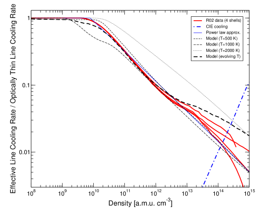
Figure 3: Ratio of cooling rates to the optically thin H₂ line cooling rate, as a function of density. The solid thick lines show the evolution of the effective (that is, as influenced by optical depth) H₂ line cooling rate as calculated by R02 in four different shells (the lowest one being the central shell), and the thick dot-dashed line shows the CIE cooling rate. The thin dashed, long dashed and dotted lines show the predictions of eq. (19) when assuming $T_{c}=500\;{\rm K}$, $1000\;{\rm K}$ and $2000\;{\rm K}$, respectively (note that these lines are not in monotonic order; the $T_{c}=500\;{\rm K}$ line actually lies between the other two); instead, the thick dashed line shows the prediction of the same equation when the temperature evolution of the central shell is kept into account. Finally, the thin solid line shows the simple power law approximation of eq. (22). All the curves making use of eq. (19) assume $\xi=0.20$.

From this result, we can obtain an average cooling rate (per unit mass) inside the “core” by estimating the total luminosity of the core as seen from outside its surface. This can be done by assuming that the “core photosphere” (the region of the core where the optical depth to the surface is $\leq 1$) radiates in the optically thin limit, while the interior (where the optical depth to the surface is $>1$) does not contribute to the total luminosity.

Since the optical depths of the various lines are different, this amounts introducing correcting factors the for cooling rate of each line into eq. (8):

$$L_{\rm lines,thick}(T)={{Xf_{\rm H_{2}}}\over{2m_{H}}}\sum_{m,n}{h\nu_{m,n}A_{m,n}\left[{{{2J_{n}+1}\over{U(T)}}e^{{E_{n}}\over{k_{\rm B}T}}}\right]}\;V_{m,n}\;G_{m,n},$$ (19)

where $V_{m,n}$ is the ratio between the volume of the “core photosphere” for the considered $(m,n)$ transition and the total core volume, given by

$$V_{m,n}=\left\{{\begin{array}[]{ll}1&\ {\rm if}\ \tau_{m,n}\leq 1\\ \left[{1-\left({1-{1\over{\tau_{m,n}}}}\right)^{3}}\right]&\ {\rm if}\ \tau_{m,n}>1.\end{array}}\right.$$ (20)

while the geometrical correction

$$G_{m,n}=\left\{{\begin{array}[]{ll}1&\ {\rm if}\ \tau_{m,n}\leq 1\\ 1-{1\over 2}\left[{{2\over{\tau_{m,n}}}\left({1-{1\over{2\tau_{m,n}}}}\right)}\right]^{1/2}&\ {\rm if}\ \tau_{m,n}>1.\end{array}}\right.$$ (21)

accounts for the radiation emitted towards the interior.

We note that both the form of $V_{m,n}$ as the ratio of the photospheric to the core volume, and the photospheric volume itself (at least in the optically thick case) clearly depend on the assumption that inside the core density and temperature are constant.

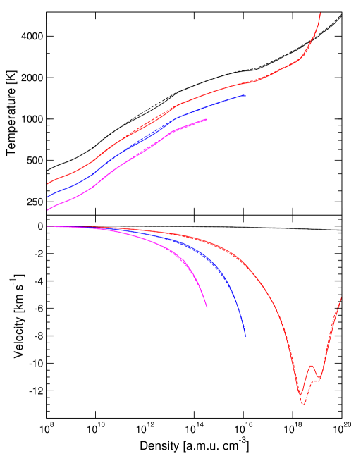
Figure 4: Comparison of the results of a modified version of the R02 code (solid lines) and of the original one (dashed lines). In the modified version the cooling rate is given by eq. (36), which is the sum of the approximate cooling rates discussed in Section 2.2.2 (H₂ lines) and in Sections 2.2.1 and 3.3 (CIE); instead, in the original code the cooling rate is estimated through radiative transfer calculations. In the top panel we compare the evolution of four shells (including the central one) in the $n-T$ plane; since all the lines were very close to each other, we artificially shifted down the results of the three non-central shells (with the bottom lines corresponding to the outermost shell). In the bottom panel we compare the evolution of the same four shells in the $n-v$ plane. Note that two of our zones do not reach the maximum density shown in these plots, so the corresponding lines stop at $n\simeq 10^{14}\;{\rm cm^{-3}}$ and $n\simeq 10^{16}\;{\rm cm^{-3}}$

In Fig. 3 we compare the results of eq. (19) to the findings of R02. Provided that a sensible value of $\xi$ is chosen (in Fig. 3 we are using $\xi=0.20$), the agreement is very good up to number densities of $n\sim 10^{13}\;{\rm cm^{-3}}$, and remains reasonable (within a factor of 2) up to the density where CIE cooling starts to be dominant ($n\sim 10^{14}\;{\rm cm^{-3}}$). The differences can be partially explained by noting that at the highest densities the $\xi$ values reported in Table 2 are substantially higher than the adopted value of 0.20. It is also remarkable that the agreement remains good also when we consider the R02 results for non-central shells, provided that their own physical properties ($T,\ n\ {\rm and}\ f_{\rm H_{2}}$) are plugged into eq. (18) instead of the central ones.

In the next sections we need an analytic expression for the cooling rate which is less cumbersome than eq. (19). We choose to employ a very simple approximation of the form

$$L_{\rm lines,thick}(T)=L_{\rm lines,thin}(T)\min{(1,(n/n_{0})^{-\beta})}$$ (22)

with $n_{0}=8\times 10^{9}\;{\rm cm^{-3}}$ (equivalent to $\rho_{0}=1.34\times 10^{-14}\;{\rm g\,cm^{-3}}$) and $\beta=0.45$.

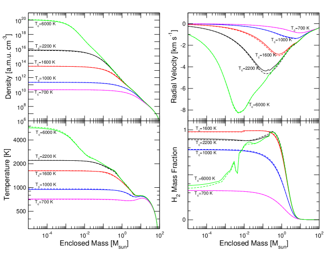
Figure 5: Comparison of the results of the original and of the modified R02 code (see caption of fig. 4). The various panels show the spatial profiles of density (top left), velocity (top right), temperature (bottom left) and molecular fraction (bottom right) at five different stages (specified through their central temperature) when the simplification in the H₂ lines cooling rate is relevant. Dashed lines show the results of the original code, while solid lines show the result of the simplified one. The spatial coordinate is specified through the Lagrangian coordinate of R02, i.e. the enclosed mass.

We have tested the validity of both equations (19) and (22) by substituting it to the radiative transfer treatment inside the code used by R02 for their simulations, and comparing the results with those of the original code; in these tests we also added an approximate CIE contribution as can be found in eq. (36). As can be seen in Fig. 4 and 5 (which show the results obtained using eq. 22), the evolution is strikingly similar, not only in the central zones but also in the outer regions. So, we have been able to predict the global effect of radiative transfer on the H₂ line cooling with a simple model based on purely local properties. It is quite remarkable (and partly unexpected) that a treatment which was believed to apply just to the centre of the “core” can be applied also to the non-central regions.

The results of eq. (19) and (22) could be used for extending full 3-D simulations to densities up to $n\sim 10^{16}\;{\rm cm^{-3}}$. However, we have to remark that such an approach is likely to be correct only if the collapsing object remains approximately spherical at all stages, and if the spatial profiles (of density, temperature, chemical composition etc.) actually resemble the 1-D results, at least until the moment when CIE cooling starts to overcome H₂ lines ($n\lower 2.15277pt\hbox{$\;\buildrel>\over{\sim}\;$}10^{14}\;{\rm cm^{-3}}$).

3 Instabilities

In this section, we investigate whether a collapsing protostellar cloud can become unstable to fragmentation by means of two different instability criteria.

3.1 Timescales comparison

A classical criterion for fragmentation is that the cooling time $t_{\rm cool}$ must be shorter that the dynamical timescale

$$t_{\rm dyn}\equiv\left({{3\pi}\over{16G\rho}}\right)^{1/2}.$$ (23)

In Fig. 6, we show the evolution of the ratios of three relevant timescales to the dynamical timescale, as determined from R02 data about the central evolution of a proto-stellar object (in the rest of this paper, we will refer to this evolutionary track as the “R02 path”).

These timescales are:
- the radiative cooling timescale (accounting for the effects of cooling)

$$t_{\rm rad}={{[1/(\mu m_{\rm H})]k_{\rm B}T}\over{L_{\rm rad}(\gamma-1)}}$$ (24)

where $L_{\rm rad}$ is the total radiative cooling rate per unit mass ($L_{\rm rad}=L_{\rm lines}+L_{\rm CIE}$ in the conditions we are considering) and $\gamma$ is the mean adiabatic index of the gas (cfr. ON98);
- the thermo-chemical timescale (accounting for the thermal effects of chemical reactions, namely of formation or disruption of H₂ )

$$t_{\rm chem}={{(n/\mu)k_{\rm B}T}\over{|\dot{E}_{\rm chem}|(\gamma-1)}}\simeq{{(n/\mu)k_{\rm B}T}\over{|\dot{n}_{\rm H_{2}}|\chi_{\rm H_{2}}(\gamma-1)}},$$ (25)

where $\dot{E}_{\rm chem}\simeq-\dot{n}_{\rm H_{2}}\chi_{\rm H_{2}}$ is the rate of variation of chemical energy (per unit volume), $\dot{n}_{\rm H_{2}}$ is the rate of H₂ formation (per unit volume) and $\chi_{\rm H_{2}}=4.48\;{\rm eV}$ is the binding energy of H₂ ;
- the “effective” cooling timescale (accounting for both chemical reactions and radiation):

$$t_{\rm cool}={{[1/(\mu m_{\rm H})]k_{\rm B}T}\over{(L_{\rm rad}-\dot{E}_{\rm chem}/\rho)(\gamma-1)}}.$$ (26)

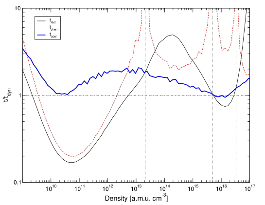
Figure 6: Evolution of the ratio of the radiative cooling timescale $t_{\rm rad}$ (thin solid line), chemical timescale $t_{\rm chem}$ (dashed line) and cooling timescale $t_{\rm cool}$ (thick solid line) to the dynamical timescale $t_{\rm dyn}$, as a function of density. The data come from the protostellar collapse simulations of R02 and refer to the central zone (“R02 path”). The three vertical dotted lines at densities $\sim 3\times 10^{13}$, $\sim 5\times 10^{15}$ and $\sim 3\times 10^{16}\;{\rm m_{H}\,cm^{-3}}$ show where the chemical heating term vanishes (implying $t_{\rm chem}=\infty$ and $t_{\rm cool}=t_{\rm rad}$) and changes sign. The horizontal dot-dashed line just visualizes the criterion $t<t_{\rm dyn}$.

It can be seen in Fig. 6 that the ratio $t_{\rm cool}/t_{\rm dyn}$ is close to 1 for most of the considered evolution, although it never really crosses this critical value. Since the above criterion is only a sufficient condition for instability, we consider a more detailed instability criterion next.

3.2 CIE induced instabilities

3.2.1 Chemo-thermal instability criterion

Silk (1983; see also Sabano & Yoshii 1977) considered a gas cloud in chemical and thermal equilibrium and investigates the conditions for the growth of isobaric perturbations. Assuming infinitesimal perturbations of the form $T=T_{1}\exp(ikx+\omega t)$, a dispersion relation

$$A\omega^{2}+B\omega+C=0$$ (27)

is obtained, which can be used to assess the stability of a given gas cloud. Similar results were obtained by Saio & Yoshii (1986), and OY03, who were able to drop the assumption of chemical and thermal equilibrium.

We use the values of the coefficients $A$, $B$ and $C$ which are given by equations (A19-A27) of OY03: they depend on the temperature $T$, on the density $\rho$, on the molecular mass fraction $f_{\rm H_{2}}$, on the two functions ${\mathcal{F}}(\rho,T,f_{\rm H_{2}})\equiv{{df_{\rm H_{2}}}\over{dt}}$ (rate of change of the molecular mass fraction) and ${\mathcal{L}}(\rho,T,f_{\rm H_{2}})$ (cooling rate per unit mass), and on their partial derivatives ${\mathcal{F}}_{\rho}=\partial{\mathcal{F}}/\partial\rho$, ${\mathcal{F}}_{f}=\partial{\mathcal{F}}/\partial f_{\rm H_{2}}$, ${\mathcal{F}}_{T}=\partial{\mathcal{F}}/\partial T$, ${\mathcal{L}}_{\rho}=\partial{\mathcal{L}}/\partial\rho$, ${\mathcal{L}}_{f}=\partial{\mathcal{L}}/\partial f_{\rm H_{2}}$, and ${\mathcal{L}}_{T}=\partial{\mathcal{L}}/\partial T$.

Since $A$ must be positive, it is possible to have growing perturbations (i.e. , ${\rm Re}(\omega)>0$) if and only if $C<0$, with (cfr. OY03, appendix A)

$$C= -{{\mu m_{\rm H}}\over{k_{\rm B}T}}(T{\mathcal{L}}_{T}-\rho{\mathcal{L}}_{\rho}-{\mathcal{L}})({\mathcal{F}}_{f}+{\mu\over 2}\rho{\mathcal{F}}_{\rho}+{{\mathcal{F}}\over{2-f_{\rm H_{2}}}})$$ (28)

$$+{{\mu m_{\rm H}}\over{k_{\rm B}T}}({\mathcal{L}}_{f}+{\mu\over 2}\rho{\mathcal{L}}_{\rho}+{1\over{6-f_{\rm H_{2}}}}{\mathcal{L}})(T{\mathcal{F}}_{T}-\rho{\mathcal{F}}_{\rho})$$

$$+{\mu\over 2}{\mathcal{F}}\left[{{\mu\over{3-f_{\rm H_{2}}/2}}({1\over 2}+{\chi\over{k_{\rm B}T}})(T{\mathcal{F}}_{T}-\rho{\mathcal{F}}_{\rho})-{\chi\over{k_{\rm B}T}}({\mathcal{F}}_{f}+{\mu\over 2}\rho{\mathcal{F}}_{\rho}+{{\mathcal{F}}\over{2-f_{\rm H_{2}}}})}\right]$$

$$+{\mu\over{(3-f_{\rm H_{2}}/2)t_{\rm ff}}}(T{\mathcal{F}}_{T}-\rho{\mathcal{F}}_{\rho}),$$

where $\mu=(1-f_{\rm H_{2}}/2)^{-1}$ is the mean molecular weight (OY03 assumed a pure H-H₂ gas) and $t_{\rm ff}=[3\pi/(32G\rho)]^{1/2}$ is the free fall timescale.

3.2.2 The H₂ formation and cooling rates (${\mathcal{F}}$ and ${\mathcal{L}}$)

We now apply the above instability criterion (eq. 28) to the density and temperature regime where optically thin CIE cooling could be dominant. For this reason, we will only consider the density range $10^{13}\;{\rm cm^{-3}}\leq n_{p}\leq 10^{17}\;{\rm cm^{-3}}$ (where $n_{p}=\rho X/m_{H}=n_{H}+2n_{\rm H_{2}}$ is the number density of protons); we will also restrict ourselves to the temperature range $400\;{\rm K}\leq T\leq 3000\;{\rm K}$, because of the limitations of the approximate cooling rate we are going to assume (eq. 5).

In this region of the density-temperature phase space, H₂ formation and dissociation proceeds through the three-body reactions described by PSS83, so that the function ${\mathcal{F}}$ can be written as

$${\mathcal{F}}\equiv{{df_{\rm H_{2}}}\over{dt}}=n_{f}[2nk_{4}(1-f_{\rm H_{2}})^{2}-k_{5}f_{\rm H_{2}}]$$ (29)

with

$$n_{f}=n_{p}\left({1-{{15f_{\rm H_{2}}}\over{16}}}\right),$$ (30)

while $k_{4}$ and $k_{5}$ (the notation comes from PSS83) are the reaction rates for the formation and disruption of H₂ , respectively. We use the PSS83 formation rate ($k_{4}$), but we modify the dissociation rate ($k_{5}$) in order to better approximate the “high density” ($n\lower 2.15277pt\hbox{$\;\buildrel>\over{\sim}\;$}10^{9}\;{\rm cm^{-3}}$) results of Martin, Schwarz & Mandy (1996):

$$k_{4}= 5.5\times 10^{-29}\,T^{-1}\quad{\rm cm^{6}\,s^{-1}}$$ (31)

$$k_{5}= 2.2\times 10^{-9}\,T^{0.2}\,e^{-{{B_{5}}\over T}}\,(1-e^{-{{C_{5}}\over T}})\quad{\rm cm^{3}\,s^{-1}}$$ (32)

where $B_{5}=51800\;{\rm K}$, $C_{5}=6000\;{\rm K}$.

At these high densities ON98 and R02 showed that we can safely assume that chemical equilibrium is attained, so that the condition ${\mathcal{F}}=0$ can be coupled with equation (29) in order to get the equilibrium H₂ fraction $f_{0}(\rho,T)$:

$$f_{0}(\rho,T)=1+{{k_{5}}\over{4n_{p}k_{4}}}\left[{1-\left({1+{{8n_{p}k_{4}}\over{k_{5}}}}\right)^{1/2}}\right].$$ (33)

However, we note that the third addendum in eq. (28) introduces a strong dependence of the value of $C$ upon the actual H₂ abundance, and that even relatively small differences (a few percent) in $f_{\rm H_{2}}$ can lead to significant discrepancies in the results, as we will show in the next subsection.

With regard to the “luminosity” ${\mathcal{L}}$, in this subsection we will neglect all forms of radiative cooling except CIE optically thin cooling. In addition, the internal energy also changes because of the thermalization of gravitational energy. Following S83, we will assume that a constant fraction $\Phi$ of the gravitational energy in bulk motion is thermalized, so that

$${\mathcal{L}}\simeq A_{\rm CIE}\rho T^{\alpha}Xf_{\rm H_{2}}-A_{\Phi}\rho^{1/2}T$$ (34)

where

$$A_{\Phi}={{{3k_{\rm B}}\over{2m_{H}}}\over{\sqrt{{3\pi}\over{32G}}}}\Phi\simeq 5.9\times 10^{4}\Phi\;{\rm erg\,cm^{1.5}\,g^{-0.5}\,K^{-1}},$$ (35)

and we have expressed the CIE cooling rate using eq. (5). As we previously remarked, this last approximation requires the gas to be predominantly molecular ($f_{\rm H_{2}}\lower 2.15277pt\hbox{$\;\buildrel>\over{\sim}\;$}0.5$); in the regions of phase space where this is not true (that is, close to the upper temperature limit of $3000\;{\rm K}$), the following results are probably inaccurate.

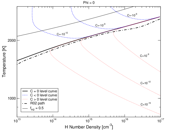
Figure 7: Value of $C$ assuming no conversion of gravitational into thermal energy ($\Phi=0$). We show the $n-T$ plane with the dashed thin contours in the unstable region corresponding to $C=-10^{-12},-10^{-9}$ and $-10^{-6}\;{\rm s^{-2}}$, the solid thick line for $C=0$, and the thin dotted contours with $C=10^{-15},10^{-12}$ and $10^{-9}\;{\rm s^{-2}}$ in the stable part of the phase diagram. The thick dot-dashed line marks the “R02 path” (the path followed by the central regions of the primordial proto–stellar cloud simulated in R02). The thin solid line, corresponding to $f_{\rm H_{2}}(\rho,T)=f_{0}(\rho,T)=0.5$, separates the low temperature region where H is mostly molecular (and eq. 5 can be used) from the high temperature region where H is mostly atomic.

3.2.3 The instability region

We examine the sign of $C$ across the $n-T$ phase space by assuming that at each point we have an equilibrium H₂ abundance (that is, $f_{\rm H_{2}}(\rho,T)=f_{0}(\rho,T)$) and that the values of ${\mathcal{F}}$ and ${\mathcal{L}}$ (and their derivatives) can be found through eqs. (29) and (34), respectively (see the appendix for the explicit expressions of the derivatives). We still need to assume a value for the $\Phi$ parameter in eq. (34), and we choose to investigate two of the most relevant values: $\Phi=0$ and $\Phi=0.5$. The former is consistent with the assumed spherical collapse scenario, while the latter is the value that can be expected if a disk in keplerian rotation forms, although such scenario is not consistent with the rest of our assumptions (for example, in a disk geometry the cooling rate is likely to be significantly higher).

In Figures 7 and 8, we show contour plots of the values of $C$ in the $n-T$ plane in the two cases.

In both plots it can be seen that at high temperatures ($T\lower 2.15277pt\hbox{$\;\buildrel>\over{\sim}\;$}1500-2500\;{\rm K}$, depending on $n$ and $\Phi$) there is a region where $C<0$ and the chemo-thermal instability can occur. Since the conversion of gravitational energy into thermal energy has a stabilizing effect, the size of the unstable region keeps reducing with increasing values of $\Phi$, but it never disappears, even when $\Phi=1$.

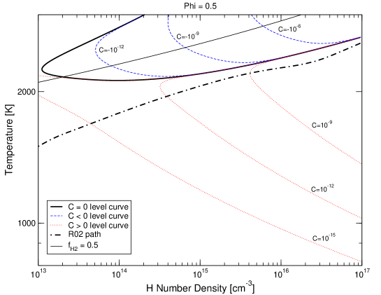
Figure 8: Same as Fig. 7, assuming a 50% conversion of gravitational into thermal energy ($\Phi=0.5$).

3.3 Instability on the R02 path

In figures 7 and 8 it is quite clear that the R02 path always remains outside the unstable region ($\Phi=0.5$), or barely grazes it ($\Phi=0$).

However, this results suffers from some important uncertainties: first of all, we already mentioned that the third addendum in eq. (28) introduces a strong dependency of $C$ on the exact value of the H₂ abundance $f_{\rm H_{2}}$ (and of its time derivative ${\mathcal{F}}$); less importantly, it only considers optically thin continuum cooling, but this is not completely appropriate at the two extremes of the considered density range.

Despite these subtleties the simple fact that the numerical results of R02 fall so close to the $C=0$ lines indicates that the presented analysis may be also applied to the collapsing proto-stellar cloud as a whole. Being able to describe the exact evolution and formation of the primordial proto-star purely analytically is highly desirable and will be the subject of a subsequent paper.

A better investigation can be accomplished by applying the same criteria described in the previous subsections to the analysis of the behaviour of the object simulated by R02 (and also by ON98). Since we have access to the full evolution of such object, we can study its properties in greater detail, and in a larger range of densities ($10^{8}\;{\rm cm^{-3}}\leq n_{p}\leq 10^{17}\;{\rm cm^{-3}}$).

First of all, we can try to fix the problems about H₂ abundance. This can be done in at least two different ways:

1. take $f_{\rm H_{2}}$ from R02 data (rather than by assuming $f_{\rm H_{2}}=f_{0}$) and leave everything else unchanged: in particular, we take the values of ${\mathcal{F}}$ and of its derivatives from eq. (29);

2. take $f_{\rm H_{2}}$ from R02 data, and also estimate values of ${\mathcal{F}}$ which are consistent with these data, but keep calculating the values of the partial derivatives ${\mathcal{F}}_{T}$, ${\mathcal{F}}_{\rho}$ and ${\mathcal{F}}_{f}$ from the analytical formulae we were using in the previous subsection.

Approach (i) is the simplest, and it is very useful at low density, where the R02 abundances are very different from the equilibrium ones because the collapsing object had not reached chemical equilibrium yet, and where both ways of estimating ${\mathcal{F}}$ (from eq. 29 and from R02 data) lead to identical results; on the other hand, at medium and high densities the results are very different (despite the small difference in the $f_{\rm H_{2}}$ values, generally just a few percent), and it must be remarked that there is a logical inconsistency in taking the H₂ abundance and its rate of variation from two different sources. From this point of view, method (ii) is clearly superior, even if not optimal: from the purely logical point of view, we should obtain also the values of ${\mathcal{F}}_{T}$, ${\mathcal{F}}_{\rho}$ and ${\mathcal{F}}_{f}$ from the R02 data, but unfortunately there is no way in which we can do that.

Fixing the luminosity term is much simpler, since we don’t have so many uncertainties: we add a term for the H₂ line luminosity into the definition of the function ${\mathcal{L}}$, and modify the CIE cooling rate by introducing a “CIE optical depth” correction factor. For the first task, we can employ the simple equation (22) combined with the Hollenbach & McKee (1979) cooling rate, while for the second we have empirically found that a correction term of the form ${{1-e^{-\tau_{c}}}\over{\tau_{c}}}$ (with $\tau_{c}=(\rho/\rho_{0,c})^{2.8}$ and $\rho_{0,c}=3.3\times 10^{-8}\;{\rm g\,cm^{-3}}$), in conjunction with a slight reduction of the normalization ($A_{\rm CIE,R02}=0.054\;{\rm erg\,cm^{3}\,g^{-2}\,s^{-1}\,K^{-4}}$, the difference is likely due to the different data set used by R02 for estimating CIE cooling) provides an excellent fit to the R02 CIE data up to the highest densities we are considering: the agreement with R02 data is actually good at least up to $n\lower 2.15277pt\hbox{$\;\buildrel>\over{\sim}\;$}10^{19}\;{\rm cm^{-3}}$ (figures 4 and 5 were obtained with this approximation). Finally, we will only consider the $\Phi=0$ case, so in the following we assume that

$${\mathcal{L}}={{Xf_{\rm H_{2}}}\over{m_{\rm H}}}{\mathcal{H}}\max{[1,(\rho/\rho_{0,l})^{-\beta_{l}}]}+A_{\rm CIE,R02}T^{\alpha}X\rho f_{\rm H_{2}}{{1-e^{-\tau_{c}}}\over{\tau_{c}}}$$ (36)

The results are shown in Fig. 9, where we show the evolution of the value of the $C$ parameter and of the corresponding instability growth timescale along the R02 path, as a function of density. The two sets of panels show the results obtained with each of the above assumptions about the values of $f_{\rm H_{2}}$ and ${\mathcal{F}}$.

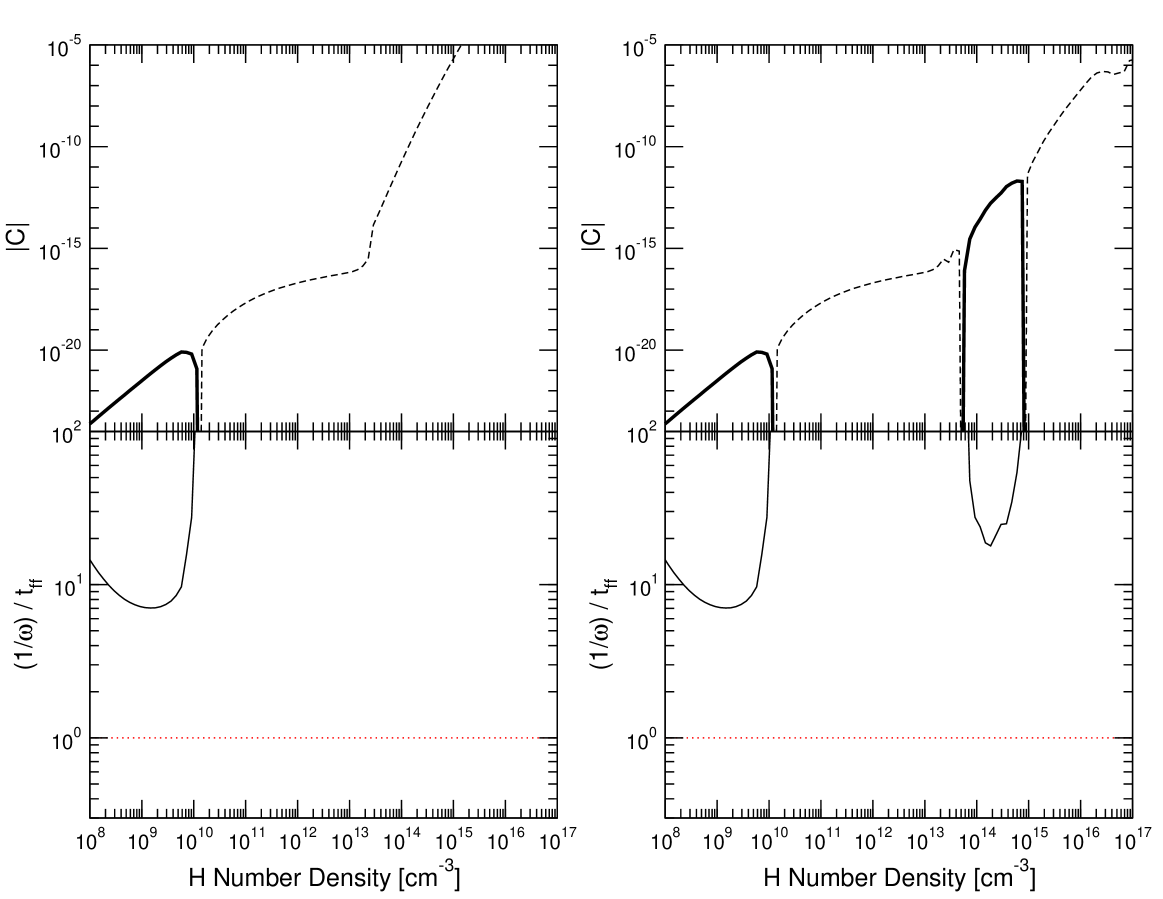
Figure 9: Value of the parameter $C$ (top panels) and of the ratio of the fluctuation growth timescale $1/\omega$ to the free-fall timescale $t_{\rm ff}$ (bottom panels) along the R02 path, with two different assumptions about the H₂ fraction variation rate ${\mathcal{F}}$. In the left panels we take the H₂ fraction $f_{\rm H_{2}}$ from the R02 results, but use the analytical values of ${\mathcal{F}}$ (case i). In the right panels we use the R02 data to get both $f_{\rm H_{2}}$ and ${\mathcal{F}}$, but we continue to estimate the derivatives of ${\mathcal{F}}$ from analytical formulae (case ii). In the upper panels, the ranges where $C<0$ (which implies instability) are denoted through a thick line, while thin dashed lines denote the ranges where $C>0$ (and the object is chemo-thermally stable). In the bottom panels we do not show this ratio when $C>0$ since that implies $\omega<0$.

First of all, it is apparent that the R02 object is unstable at low densities ($n\lower 2.15277pt\hbox{$\;\buildrel<\over{\sim}\;$}2\times 10^{10}\;{\rm cm^{-3}}$), and this is independent from the assumptions about ${\mathcal{F}}$. This regime, where the instability is due to the fast H₂ formation at the onset of 3-body reactions, corresponds to the one found by PSS83 and S83, and recently discussed by ABN02 and OY03. However, the bottom panels clearly show that the instability growth timescale is always significantly longer than the free-fall timescale, so that this kind of instability cannot actually lead to fragmentation. This result is slightly different from the one recently obtained by OY03, who find that there exists a density range about $n\simeq 5\times 10^{9}\;{\rm cm^{-3}}$ where the growth timescale is slightly shorter than the free fall one, but their conclusion (the instability is present but does not lead to fragmentation) is the same as ours. A different interpretation for the lack of fragmentation is the one pointed out by ABN02, that is, mixing due to turbulent motions: if these turbulent motions move at about the speed of sound $c_{s}$, they should be able to erase any fluctuation of size $\lower 2.15277pt\hbox{$\;\buildrel<\over{\sim}\;$}c_{s}/\omega$, and we find that the “core” where fluctuations could develop is always several times smaller than that.

The second result is that CIE cooling can lead to an instability, at least if we estimate ${\mathcal{F}}$ from the R02 data (second approach): the instability occurs over about one order of magnitude in density, when continuum optically thin cooling is dominant. However, the bottom panels show that a situation similar to the one described at low density is very likely to occur: the instability growth timescale is always much longer than the free fall timescale, and fluctuations cannot be large enough to survive turbulent mixing. We also conducted some experiments taking reasonable guesses at the values of ${\mathcal{F}}_{T}$, ${\mathcal{F}}_{\rho}$ and ${\mathcal{F}}_{f}$, with the result that the unstable range could extend over the whole phase when the cooling is due to optically thin continuum emission, but the fluctuation growth is always too slow to produce fragmentation.

4 Discussion and Conclusions

We have investigated the chemical and thermal instabilities of primordial metal-free gas during its collapse towards the formation of a protostar. We have focused on the Collision Induced Emission (CIE) and on its effects on fragmentation. We point out that even when H₂ line cooling becomes optically thick at densities $n\lower 2.15277pt\hbox{$\;\buildrel>\over{\sim}\;$}10^{10}\;{\rm cm^{-3}}$ this does not necessarily set a minimum mass scale for fragmentation due to an opacity limit. At higher densities ($n\lower 2.15277pt\hbox{$\;\buildrel>\over{\sim}\;$}10^{14}\;{\rm cm^{-3}}$) the optically thin continuum (CIE) cooling dominates, and the collapsing protostellar cloud can once again fulfill the necessary (but not sufficient) fragmentation criterion $t_{\rm cool}<t_{\rm dyn}$. We present accurate approximations to cooling and chemical rates that are particularily useful for analytical studies. A detailed analysis of the chemo–thermal stability of collapsing primordial gas leads us to conclude that the thermal instability arising from optically thin continuum cooling is of similar strength as the three body H₂ formation instability discussed previously (PSS83; S83; OY03). However, our analytical analysis of the low density instability confirms the full 3D simulations results of Abel et al. (2002) in showing that formally the instability is very strong yet it cannot grow sufficiently fast to lead to independently collapsing fragments. In hindsight, it may not be too surprising that this instability does not lead to fragmentation. It fulfills the necessary (but not sufficient) condition of leading to a cooling time shorter than the dynamical time. An unstable patch of gas will, however, grow initially only iso–barically as it is compressed from the surrounding higher pressure regions. So although the cooling rate can increase dramatically as one increases the H₂ fraction by a factor one thousand the minimum temperature the gas cools to cannot. Consequently, correspondingly small density fluctuations are formed which do not become gravitationally unstable and become mixed back in into the slightly warmer surrounding regions.

Given the efficiency of collision induced emission cooling (Figure 1) and its relatively small effect on the temperature in the one dimensional results one is tempted to conclude that it will also not lead to fragmentation. This is most likely a fair assessment since again the growth times are long and the initial iso–baric growth leads to only small overdensities. However, in a fully three–dimensional calculation the CIE cooling might be able to cool a disk forming around the primordial proto–star sufficiently far in order to become gravitationally unstable and form stellar, or even planetary size companions (see e.g. Boss 1993 and Boss 2002). Given the dramatic accretion rates of these proto–stars, however, it is not clear whether a sufficiently massive disk may form in the first place preventing a conclusive answer.

Despite the simplicity of our derivation the analytical rates for the H₂ line cooling rate in the optically thick regime and optically thick continuum cooling they are in remarkably good agreement with the radiative transfer calculations of R02 and ON98 that followed the detailed transfer of hundreds of molecular hydrogen rotational and vibrational lines. We have shown that implementing these simple approximations into the one dimensional Lagrangian hydrodynamics code developed by R02 leads to virtually indistinguishable results over all relevant density and temperature ranges. This clearly demonstrates that at least in the initial phases of primordial proto–stellar formation the effects of radiative transfer are in essence a local correction to cooling rather than a transport of energy to distant regions of the hydrodynamic flow. This is an important result which, given the analytical and purely local cooling correction factors derived here should one allow to follow the proto–stellar collapse in three dimensions all the way to stellar densities employing the recently developed versions of 128bit adaptive mesh refinement techniques of Bryan, Abel & Norman (2001) or similar high dynamic range hydrodynamic codes.

Aknowledgements

We thank K. Omukai for useful discussions and for providing us preliminary version of his OY03 paper. This work has been supported in part by the NSF CAREER award-#AST-0239709.

Appendix A Summary of Formulae and Derivatives

A.1 Luminosity

The luminosity per unit mass ${\mathcal{L}}$ can be written as (see eq. 36)

$${\mathcal{L}}\simeq{{Xf_{\rm H_{2}}}\over{m_{\rm H}}}{\mathcal{H}}\max{[1,(\rho/\rho_{0,l})^{-\beta_{l}}]}+A_{\rm CIE,R02}T^{\alpha}X\rho f_{\rm H_{2}}{{1-e^{-\tau_{c}}}\over{\tau_{c}}}-A_{\Phi}T\rho^{1/2},$$ (37)

where we have included the thermalization of gravitational energy term. The constants values are $\rho_{0,l}=1.34\times 10^{-14}\;{\rm g\,cm^{-3}}$, $\beta_{l}=0.45$, $A_{\rm CIE,R02}=0.054\;{\rm erg\,cm^{3}\,g^{-2}\,K^{-4}}$, $\alpha=4$, $\tau_{c}=(\rho/\rho_{0,c})^{2.8}$ ($\rho_{0,c}=3.3\times 10^{-8}\;{\rm g\,cm^{-3}}$) and $A_{\Phi}=5.9\times 10^{4}\;{\rm erg\,cm^{1.5}\,g^{-0.5}\,K^{-1}}$; ${\mathcal{H}}(T_{3})$ is given by eq. (7).

If the collapsing object remains approximately spherical, this formula is reasonably accurate up to densities $\rho\simeq 2\times 10^{-5}\;{\rm g\,cm^{-3}}$.

Because of the maximum in the H₂ lines term, it is useful to distinguish two cases.

if $\rho\leq\rho_{0,l}$, the partial derivatives of ${\mathcal{L}}$ are

$${\mathcal{L}}_{T}= {{\partial{\mathcal{L}}}\over{\partial T}}= {{Xf_{\rm H_{2}}}\over{m_{\rm H}}}{{\partial{\mathcal{H}}}\over{\partial T}}+\alpha A_{\rm CIE}T^{\alpha-1}X\rho f_{\rm H_{2}}{{1-e^{-\tau_{c}}}\over{\tau_{c}}}-A_{\Phi}\rho^{1/2}$$ (38)

$${\mathcal{L}}_{\rho}= {{\partial{\mathcal{L}}}\over{\partial\rho}}= A_{\rm CIE}T^{\alpha}Xf_{\rm H_{2}}\left[{\beta_{c}e^{-\tau_{c}}+(1-\beta_{c}){{1-e^{-\tau_{c}}}\over{\tau_{c}}}}\right]-{1\over 2}A_{\Phi}T\rho^{-1/2}$$ (39)

$${\mathcal{L}}_{f}= {{\partial{\mathcal{L}}}\over{\partial f_{\rm H_{2}}}}= {{X}\over{m_{\rm H}}}{\mathcal{H}}+A_{\rm CIE}T^{\alpha}X\rho{{1-e^{-\tau_{c}}}\over{\tau_{c}}}$$ (40)

Instead, if $\rho_{0,l}\leq\rho$ we have:

$${\mathcal{L}}_{T}= {{Xf_{\rm H_{2}}}\over{m_{\rm H}}}{{\partial{\mathcal{H}}}\over{\partial T}}(\rho/\rho_{0,l})^{-\beta_{l}}+\alpha A_{\rm CIE}T^{\alpha-1}X\rho f_{\rm H_{2}}{{1-e^{-\tau_{c}}}\over{\tau_{c}}}-A_{\Phi}\rho^{1/2}$$ (41)

$${\mathcal{L}}_{\rho}= -{{\beta_{l}}\over{\rho_{0,l}}}{{Xf_{\rm H_{2}}}\over{m_{\rm H}}}{\mathcal{H}}(\rho/\rho_{0,l})^{-(\beta_{l}+1)}+A_{\rm CIE}T^{\alpha}Xf_{\rm H_{2}}\left[{\beta_{c}e^{-\tau_{c}}+(1-\beta_{c}){{1-e^{-\tau_{c}}}\over{\tau_{c}}}}\right]-{1\over 2}A_{\Phi}T\rho^{-1/2}$$ (42)

$${\mathcal{L}}_{f}= {{X}\over{m_{\rm H}}}{\mathcal{H}}(\rho/\rho_{0,l})^{-\beta_{l}}+A_{\rm CIE}T^{\alpha}X\rho{{1-e^{-\tau_{c}}}\over{\tau_{c}}}$$ (43)

where, in both cases,

$${{\partial{\mathcal{H}}}\over{\partial T}}={{\partial T_{3}}\over{\partial T}}{{\partial{\mathcal{H}}}\over{\partial T_{3}}}={{10^{-3}}\over{T_{3}^{2}}}\left[{\left({{9.5\times 10^{-22}T_{3}^{3.76}}\over{1+0.12T_{3}^{2.1}}}\right)e^{-\left({{0.13}\over{T_{3}}}\right)^{3}}\left({{{3.76T_{3}+0.2T_{3}^{3.1}}\over{1+0.12T_{3}^{2.1}}}+{{0.0066}\over{T_{3}^{2}}}}\right)}\right]+$$

$$+{{10^{-3}}\over{T_{3}^{2}}}\left[{1.5\times 10^{-24}e^{-{{0.51}\over{T_{3}}}}+3.9\times 10^{-18}e^{-{{5.86}\over{T_{3}}}}+1.9\times 10^{-17}e^{-{{11.7}\over{T_{3}}}}}\right]\quad{\rm erg\,s^{-1}\,K^{-1}}$$ (44)

A.2 H₂ Formation

The H₂ formation function is given by

$${\mathcal{F}}={{\partial{f_{\rm H_{2}}}}\over{\partial t}}=n_{f}[2n_{\rm p}k_{4}(1-f_{\rm H_{2}})^{2}-k_{5}f_{\rm H_{2}}]$$ (45)

where

$$n_{\rm p}\equiv\rho X/m_{\rm H},\qquad n_{f}=n_{\rm p}(1-15f_{\rm H_{2}}/16)$$ (46)

and (as explained in section 3.2.2)

$$k_{4}=A_{4}T^{-1},\qquad k_{5}=A_{5}T^{0.2}e^{-B_{5}/T}(1-e^{-C_{5}/T}),$$ (47)

with $A_{4}=5.5\times 10^{-29}\;{\rm cm^{6}\,s^{-1}}$, $A_{5}=2.2\times 10^{-9}\;{\rm cm^{3}\,s^{-1}}$, $B_{5}=51800\;{\rm K}$, $C_{5}=6000\;{\rm K}$.

The partial derivatives are

$${\mathcal{F}}_{T}\equiv {{\partial{\mathcal{F}}}\over{\partial T}}= -{{n_{f}}\over T}\left[{2n_{\rm p}k_{4}(1-f_{\rm H_{2}})^{2}+k_{5}f_{\rm H_{2}}\left({0.2+{{B_{5}}\over T}+{{C_{5}}\over T}{1\over{e^{C_{5}/T}-1}}}\right)}\right]$$ (48)

$${\mathcal{F}}_{\rho}\equiv {{\partial{\mathcal{F}}}\over{\partial\rho}}= {{n_{f}}\over\rho}[4n_{\rm p}k_{4}(1-f_{\rm H_{2}})^{2}-k_{5}f_{\rm H_{2}}]$$ (49)

$${\mathcal{F}}_{f}\equiv {{\partial{\mathcal{F}}}\over{\partial f_{\rm H_{2}}}}= -n_{f}\left\{{{{15}\over{16-15f}}[2n_{\rm p}k_{4}(1-f_{\rm H_{2}})^{2}-k_{5}f_{\rm H_{2}}]+4n_{\rm p}k_{4}(1-f_{\rm H_{2}})+k_{5}}\right\}$$ (50)

References

- [1] Abel T., Anninos P., Norman M.L., Zhang Y., 1998, ApJ, 508, 518
- [2] Abel T., Bryan G.L., Norman M.L., 2000, ApJ 540, 39
- [3] Abel T., Bryan G.L., Norman M.L., 2002, Science, 295, 93 [ABN02]
- [4] Bonnor W.B., 1956, MNRAS, 116, 351
- [5] Borysow A., Jorgensen U.G., Fu Y., 2001, JQSRT, 68, 235
- [6] Borysow A., 2002, A&A, 390, 779
- [7] Boss A.P., 1993, ApJ, 410, 157
- [8] Boss A.P., 2002, ApJ, 567, L149
- [9] Bromm V., Coppi P.S., Larson R.B., 2002, ApJ, 564, 23
- [10] Bryan G.L., Abel T., Norman M.L., 2001, in Proc. ACM/IEEE Conf. on Supercomputing (CD-ROM; New York: ACM Press), 13
- [11] Couchman, H. M. P. & Rees, M. J. 1986, MNRAS, 221, 53
- [12] Ebert R., 1955, Zs. Ap., 217
- [13] Frommhold L., 1993, Collision-induced absorption in gases, Cambridge University Press, Cambridge (UK)
- [14] Fuller T.M., Couchman H.M.P., 2000, ApJ, 544, 6
- [15] Galli D., Palla F., 1998, A&A, 335, 403
- [16] Gustafsson M., Frommhold L., 2001, ApJ 546, 1168
- [17] Gustafsson M., Frommhold L., Meyer W., 2003, Journal of Chemical Physics, 118, 1667
- [18] Jorgensen U.G., Hammer D., Borysow A., Falkesgaard J., 2000, A&A, 361, 283
- [19] Larson R.B., 1969, MNRAS, 145, 271
- [20] Lenzuni P., Chernoff D.F., Salpeter E.E., 1991, ApJS, 76, 759
- [21] Lepp S., Shull J.M., 1983, ApJ, 270, 578
- [22] Machacek M.E., Bryan G.L., Abel T., 2001, ApJ, 548, 509
- [23] Martin P.G., Schwarz D.H., Mandy M.E., 1996, ApJ, 461, 265
- [24] Nishi R., Susa H., 1999, ApJ, 523, 103
- [25] Omukai K., Nishi R., 1998, ApJ, 508, 141 [ON98]
- [26] Omukai K., Yoshii Y., 2003, ApJ, accepted (astro-ph/0308514) [OY03]
- [27] Palla F., Salpeter E.E., Stahler S.W., 1983, ApJ, 271, 632
- [28] Penston M.V., 1969, MNRAS, 144, 425
- [29] Rees M.J., 1976, MNRAS, 176, 483
- [30] Ripamonti E., Haardt F., Ferrara A., Colpi M., 2002, MNRAS 334, 401 [R02]
- [31] Sabano Y., Yoshii Y., 1977, PASJ, 29, 207
- [32] Saio H., Yoshii Y., 1986, ApJ, 301, 587
- [33] Silk J., 1983, MNRAS, 205, 705 [S83]
- [34] Tegmark M., Silk J., Rees M., Blanchard A., Abel T., Palla F., 1997, ApJ, 474, 1