On the Measurement of the Magnitude and Orientation of the Magnetic Field in Molecular Clouds.

Abstract

We demonstrate that the combination of Zeeman, polarimetry and ion-to-neutral molecular line width ratio measurements permits the determination of the magnitude and orientation of the magnetic field in the weakly ionized parts of molecular clouds. Zeeman measurements provide the strength of the magnetic field along the line of sight, polarimetry measurements give the field orientation in the plane of the sky and the ion-to-neutral molecular line width ratio determines the angle between the magnetic field and the line of sight. We apply the technique to the M17 star-forming region using a HERTZ 350 $\mu$m polarimetry map and HCO⁺-to-HCN molecular line width ratios to provide the first three-dimensional view of the magnetic field in M17.

1 Introduction

In this paper, we propose a method that will permit the determination of the magnitude and orientation of the magnetic field in the weakly ionized parts of molecular clouds. As it turns out, the magnetic field can be specified with three parameters: its magnitude $B$, the viewing angle $\alpha$ defining its orientation relative to the line of sight and the angle $\beta$ made by its projection on the plane of the sky (as defined relative to a predetermined direction, east from north, see Figure 1). Up till now, of these three quantities only the third could be measured. At submillimeter wavelengths, this can be accomplished, for example, with polarization measurements of the continuum radiation emanating from elongated dust grains that are aligned by the local magnetic field (Davis & Greenstein, 1952). The angle $\beta$ is thus obtained from the angle of the polarization vector. The projection of the magnetic field vector in the plane of the sky is oriented at right angles to the polarization vector (Hildebrand, 1988). The magnitude $B$ cannot be directly measured, only the projection of the magnetic field vector to the line of sight $B_{los}$ can be obtained with Zeeman measurements. Despite the inherent difficulties associated with this technique, numerous molecular clouds have lately been successfully studied using measurements of interstellar lines from the HI, OH and CN species (e.g., Brogan & Troland (2001); Brogan et al. (1999); Crutcher et al. (1993, 1999); Heiles (1997)). For general cases, where the magnetic field lies out of the plane of the sky, a determination of the viewing angle $\alpha$, in combination with the measurements for $B_{los}$ and $\beta$, would provide a description of the magnetic field vector $\mathbf{B}$. Up to now, this has been impossible to achieve.

Starting with the next section, we will show how the determination of the viewing angle $\alpha$ can be accomplished through a comparison of the profile of line spectra from coexistent ion and molecular species (we will use HCO⁺ and HCN). Our analysis will be based on the material presented by Houde et al. (2000a, b) and we will show that the ion-to-neutral line width ratio, as defined by these authors, is a fundamental parameter and holds the key to the determination of the viewing angle. We will then apply and test our new technique with data obtained for the M17 molecular cloud. More precisely, we will combine our HCO⁺ and HCN spectroscopic data with an extensive 350 $\mu$m continuum polarimetry map obtained with the HERTZ polarimeter (Dowell et al., 1998) at the Caltech Submillimeter Observatory (CSO) to provide the first three-dimensional view of the magnetic field in M17.

In this paper, we will focus more on the presentation and the discussion of our technique, rather than the interpretation of the magnetic field results for M17. That aspect will be treated in a subsequent paper.

2 The ion-to-neutral line width ratio

Houde et al. (2000a, b) have recently shown how a comparison of the line profiles of coexistent neutral and ion species can be used to detect the presence of the magnetic field in molecular clouds. Assuming a weakly ionized plasma, elastic collisions and the presence of neutral flows or turbulence in the region under study, they arrived at the conclusion that, in the core of molecular clouds, the width of line profiles of molecular ions should in general be less than that of coexistent neutral molecular species.

In considering an idealized situation where they investigated the behavior of an isolated ion subjected to the presence of a neutral flow, they found the following equations for the mean and variance of its velocity components

$$\left\langle\mathbf{v}_{\|,i}\right\rangle = \left\langle\mathbf{v}_{\|,n}\right\rangle$$ (1)

$$\left\langle\mathbf{v}_{\bot,i}\right\rangle = \frac{\left\langle\mathbf{v}_{\bot,n}\right\rangle+\left\langle\omega_{r,i}\right\rangle^{-1}\left[\left\langle\mathbf{v}_{\bot,n}\right\rangle\times\left\langle\overrightarrow{\omega}_{g,i}\right\rangle\right]}{1+\left(\frac{\left\langle\omega_{g,i}\right\rangle}{\left\langle\omega_{r,i}\right\rangle}\right)^{2}}$$ (2)

$$\sigma_{\|,i}^{2} = \frac{a\left[\left\langle\mathbf{v}_{\bot,n}^{2}\right\rangle-\left\langle\mathbf{v}_{\bot,i}\right\rangle^{2}\right]+b\,\sigma_{\|,n}^{2}}{\left[\frac{m_{i}}{\mu_{i}}-1\right]}$$ (3)

$$\sigma_{\bot,i}^{2} = \frac{g\left[\left\langle\mathbf{v}_{\bot,n}^{2}\right\rangle-\left\langle\mathbf{v}_{\bot,i}\right\rangle^{2}\right]+h\,\sigma_{\|,n}^{2}}{\left[\frac{m_{i}}{\mu_{i}}-1\right]}$$ (4)

$$\sigma_{T,i}^{2} = \frac{\left[\left\langle\mathbf{v}_{\bot,n}^{2}\right\rangle-\left\langle\mathbf{v}_{\bot,i}\right\rangle^{2}\right]+\sigma_{\|,n}^{2}}{\left[\frac{m_{i}}{\mu_{i}}-1\right]}$$ (5)

with

$$\left\langle\overrightarrow{\omega}_{g,i}\right\rangle = \frac{e\left\langle\mathbf{B}\right\rangle}{m_{i}c}$$ (6)

$$\left\langle\omega_{r,i}\right\rangle \simeq \frac{\mu_{i}}{m_{i}}\nu_{c,i}$$ (7)

$$\sigma_{T,n}^{2} = \left\langle\mathbf{v}_{n}^{2}\right\rangle-\left\langle\mathbf{v}_{n}\right\rangle^{2}\,,$$ (8)

where $m_{i}$ and $\mu_{i}$ are the ion mass and reduced mass, respectively. The ion and neutral flow velocities ($\mathbf{v}_{i}$ and $\mathbf{v}_{n}$) were broken into two components: one parallel to the magnetic field ($\mathbf{v}_{\|,i}$ and $\mathbf{v}_{\|,n}$) and another ($\mathbf{v}_{\bot,i}$ and $\mathbf{v}_{\bot,n}$) perpendicular to it. $\left\langle\omega_{r,i}\right\rangle$, $\left\langle\overrightarrow{\omega}_{g,i}\right\rangle$ and $\nu_{c,i}$ are the ion relaxation rate, mean gyrofrequency vector and collision rate, respectively. Under the assumption that the neutral flow consists mainly of molecular hydrogen and has a mean molecular mass $A_{n}=2.3$, we get $a\simeq 0.16$, $b\simeq 0.67$, $g=1-a$ and $h=1-b$.

It was the study of this set of equations that lead Houde et al. (2000a) to the conclusion that the presence of a magnetic field in the weakly ionized part of molecular clouds will generally lead to ion molecular line profiles of narrower width when compared to those of coexistent neutral species. This fact was expressed more quantitatively in their subsequent paper (Houde et al., 2000b) where expressions for the ion and neutral line widths were derived for the special case where the region under consideration has an azimuthal symmetry about the axis defined by the direction of the magnetic field and a reflection symmetry across the plane perpendicular to this axis. In such instances, the line widths ($\sigma_{l,n}$ and $\sigma_{l,i}$ for the neutrals and ions, respectively) can be expressed by their variance as

$$\sigma_{l,n}^{2} = \sum_{k}C^{k}\left\langle\mathbf{v}_{n}^{k}\right\rangle^{2}\left[\cos^{2}\left(\theta^{k}\right)\cos^{2}\left(\alpha\right)+\frac{1}{2}\sin^{2}\left(\theta^{k}\right)\sin^{2}\left(\alpha\right)\right]$$ (9)

$$\sigma_{l,i}^{2} \simeq \sum_{k}C^{k}\left\langle\mathbf{v}_{n}^{k}\right\rangle^{2}\left[\rule{0.0pt}{21.52771pt}\cos^{2}\left(\theta^{k}\right)\cos^{2}\left(\alpha\right)\right.$$ (10)

$$\left.+\frac{\sin^{2}\left(\theta^{k}\right)}{\left[\frac{m_{i}}{\mu_{i}}-1\right]}\left[a\cos^{2}\left(\alpha\right)+\frac{g}{2}\sin^{2}\left(\alpha\right)\right]\right]\,,$$

where it was assumed that the different neutral flows, of velocity $\mathbf{v}_{n}^{k}$ at an angle $\theta^{k}$ relative to the axis of symmetry, do not have any intrinsic dispersion. The term $C^{k}$ is the weight associated with the neutral flow $k$, which presumably scales with the particle density (we assume that ions and neutrals exist in similar proportions). An example of such a configuration is shown in Figure 2. It is important to realize that although the type of geometry presented in this figure (a bipolar outflow) has the aforementioned characteristics, we are not limited to this model. What matters is the relative orientation of the individual neutral flows and not their position in space, i.e., all the flows shown in Figure 2 could be arbitrarily repositioned and equations (9) and (10) would still apply (as long as all the flows are contained in the region under study).

An important feature that can be assessed from equations (9) and (10) is that the line width ratio $\sigma_{l,i}/\sigma_{l,n}$ is not only a function of the orientation of the neutral flows but also of the viewing angle $\alpha$. It is easy to show that $\sigma_{l,n}\simeq\sigma_{l,i}$ when the magnetic field is oriented parallel to the line of sight (i.e., when $\alpha=0$) and that the line width ratio is minimum when the magnetic field is in the plane of the sky (when $\alpha=\pi/2$) with

$$\frac{\sigma_{l,i}}{\sigma_{l,n}}\simeq\left[\frac{g}{\frac{m_{i}}{\mu_{i}}-1}\right]^{\frac{1}{2}}\simeq 0.26$$

for HCO⁺ (with $\theta^{k}\neq 0$ for at least one value of $k$ (Houde et al., 2001)).

We present in Table 1 the line width ratios measured for a relatively large sample of molecular clouds. As can be seen, with the exception of HH 7-11 and Mon R2 which have ratios of very nearly unity, every source shows the ion molecular species as having a narrower line width than the corresponding coexistent neutral species.

This aspect is made even more evident by studying Figure 3 where we plotted the ion line width against the corresponding neutral line width for every object and pair of molecular species studied so far (HCO⁺ is plotted against HCN and H¹³CO⁺ against H¹³CN). The two straight lines correspond to the upper and lower limits discussed above, the steeper of the two (with a slope of $\simeq 1$) arises when the magnetic field is oriented in a direction parallel to the line of sight while the other (with a slope of $\simeq 0.26$) when the field lies in the plane of the sky. As can be readily seen from this figure, the data obtained so far is in excellent agreement with Houde et al.’s model and the prediction it makes. Even the lower limit of $\simeq 0.26$ for the line width ratio predicted by the simple model defined earlier appears to be fairly accurate as only two of the more than ninety plotted points have a ratio which is lower than this value, and then only slightly.

These results have important implications for the study of the magnetic field in molecular clouds. Namely:

1. In the weakly ionized regions of turbulent molecular clouds, the neutrals drive the ions. If the opposite were true, we would expect the ion species to exhibit line profiles which would be at least as broad as those of coexistent neutral species and probably broader (Houde et al., 2001), contrary to observation.

2. The difference in the width of the line profiles of coexistent ion and neutral molecular species implies that the coupling between ions and neutrals is poor in the core of molecular clouds, at least at the scales probed by our observations (up to a few tenths of a parsec).

3. At the spatial resolution attained with our observations (we have a beam width of $\approx 20\arcsec$ in most cases), the diffusion between ions and neutrals can be studied through a comparison of the width of their line profiles. It then appears from our results that the drift speed between ions and neutrals can often be significant in the core of molecular clouds (on the order of a few km/s at the gas densities probed with the molecular species used here, i.e., $n\gtrsim 10^{6}$ cm^-3).

3 The determination of the viewing angle $\alpha$

From our previous discussion leading to equations (9) and (10) and the determination of the upper and lower limits for the line width ratio, one might infer that this parameter could possibly convey important information about the angle $\alpha$ that the magnetic field makes relative to the line of sight. More precisely, since the line width ratio is maximum at approximately unity when the field is aligned with the line of sight ($\alpha=0$) and decreases to a minimum of $\simeq 0.26$ when the field lies in the plane of the sky ($\alpha=\pi/2$), we could be justified in hoping that it might be a well-behaved function which decreases monotonically with increasing $\alpha$.

We can explore this proposition by using our earlier model of symmetrical neutral flow configuration. For example, we could define cases with different amounts of collimation for the neutral flows around the axis of symmetry specified by the orientation of the magnetic field. An example was shown in Figure 2 where all the neutral flows are contained within a cone of angular width $\Delta\theta$. Using such a model, with the additional simplification that the neutral flow angle $\theta^{k}$ is independent of the velocity $v_{n}^{k}$, theoretical line widths $\sigma_{l,n}$ and $\sigma_{l,i}$ can be calculated for different values of $\Delta\theta$ using equations (9) and (10). We then get for the square of the ratio

$$\frac{\sigma_{l,i}^{2}}{\sigma_{l,n}^{2}} \simeq \frac{e\cos^{2}\left(\alpha\right)+f\left[a\cos^{2}\left(\alpha\right)+g\sin^{2}\left(\alpha\right)/2\right]\left[\frac{m_{i}}{\mu_{i}}-1\right]^{-1}}{e\cos^{2}\left(\alpha\right)+f\sin^{2}\left(\alpha\right)/2}$$ (11)

with

$$e = \left[1-\cos^{3}\left(\Delta\theta\right)\right]/6$$

$$f = \left[2-3\cos\left(\Delta\theta\right)+\cos^{3}\left(\Delta\theta\right)\right]/6\,.$$

Examples of such models are shown in Figure 4 where the line width ratio is plotted against the viewing angle $\alpha$ for neutral flow collimation widths of $20^{\circ}$, $40^{\circ}$, $60^{\circ}$ and $90^{\circ}$ (no collimation). Note that every curve is monotonic and has a ratio of $\simeq 1$ at $\alpha=0$ and $\simeq 0.26$ at $\alpha=\pi/2$ as was determined earlier. This implies that it would be, in principle, possible to determine the viewing angle as a function of the line width ratio if we knew the curve (or the amount of collimation) which corresponds best to the object or region under study. We next show how this can be done.

3.1 Line width ratio vs polarization level

As it turns out, there exists another parameter that is a function of the orientation of the magnetic field relative to the line of sight that can be readily obtained. This is the polarization level that is measured, for example, from the continuum emission from dust at submillimeter wavelengths. Indeed, since the (elongated) dust grains are presumably aligned by the magnetic field, the polarization level $P$ detected by an observer studying a given region where the field is oriented with a viewing angle $\alpha$ can be expressed as

$$P=P_{max}\sin^{2}\left(\alpha\right)\,,$$ (12)

where $P_{max}$ is the maximum polarization level that can be detected, i.e. when the field lies in the plane of the sky ($\alpha=\pi/2$). Evidently equation (12) can be inserted in equations (9) and (10) to eliminate $\sin^{2}\left(\alpha\right)$ and express the ion-to-neutral line width ratio as a function of the normalized polarization level $P/P_{max}$. Figure 5 shows the relationship between those two parameters for the same four cases presented in Figure 4. Given the appropriate model for the neutral flow collimation, we would then expect a set of data (of the ion-to-neutral line width ratio vs normalized polarization level) to fall along the corresponding curve. Or should we?

It is now well known that submillimeter (or far-infrared) polarization maps of molecular clouds usually show that the polarization level decreases toward regions of higher optical depth. This decrease in polarization is more than what could be expected from opacity effects and is not correlated with the dust temperature (Dotson, 1996; Weintraub, Goodman and Akeson, 2000). Even though this phenomenon is poorly understood, there is some evidence that it is caused by either small-scale fluctuations in the magnetic field (Rao et al., 1998), decrease in grain alignment with increasing optical depth or spherical grain growth. In view of this, we should not expect data (of ion-to-neutral line width ratio against normalized polarization level) to fall along a given curve, as shown in Figure 5, but rather within an area bounded by the $P/P_{max}=0$ limit and the curve in question (for this, we use a value of $P_{max}$ that would be found in a region that is unaffected by the depolarization effect). This is shown in Figure 5 for the model with a neutral flow collimation of $\Delta\theta=90^{\circ}$ where the shaded region represents the area where we now expect the data to fall. Locations in a molecular cloud that are greatly affected by the depolarization effect will tend to lie closer to the $P/P_{max}=0$ boundary whereas those that are little or not affected should fall close to theoretical curve (with $\Delta\theta=90^{\circ}$ in this example).

Still, the curve that best fits a given set of data can be used to determine the viewing angle $\alpha$ as a function of the ion-to-neutral line width ratio. Once this curve is identified, one merely has to invert the corresponding curve plotted in Figure 4 (or equation (11)) starting with the line width ratio to obtain $\alpha$. For cases where the field lies out of the plane of the sky, this information can in turn be combined with Zeeman and polarimetry measurements to determine the magnitude and the orientation of the magnetic field (the orientation of the field is not completely determined since there is an ambiguity of 180^∘ in the value of the angle $\beta$ obtained from polarimetry).

3.2 The nature of $\alpha$

It is appropriate at this time to be more precise in defining the nature of the angle $\alpha$ in relation to actual measurements made in molecular clouds. All the equations presented so far dealt with a single mean component for the magnetic field $\left\langle\mathbf{B}\right\rangle$ at a given point in space (and time) within a molecular cloud and its effect on the behavior of ions. The viewing angle $\alpha$ was then defined in relation to this mean field as follows

$$\left\langle\mathbf{B}\right\rangle=\left\langle B\right\rangle\left[\cos\left(\alpha\right)\mathbf{e}_{\|}+\sin\left(\alpha\right)\mathbf{e}_{\bot}\right]\,.$$

However, since observations are done with a finite resolution it is likely that the magnetic field could change orientation or that numerous magnetic field components $\left\langle B_{i}\right\rangle$ could be present within the region of the molecular clouds subtended by the telescope beam width, and contribute equally in shaping the line profile of molecular ion species. Under such circumstances, equation (10) for the ion line width and subsequently equation (11) for the ion-to-neutral line width ratio can easily be modified to take this into account. This is done by simply replacing $\cos^{2}\left(\alpha\right)$ and $\sin^{2}\left(\alpha\right)$ in these equations by their average over all the components, namely

$$\cos^{2}\left(\alpha\right) \rightarrow \left\langle\cos^{2}\left(\alpha\right)\right\rangle=\frac{1}{N}\sum_{i=1}^{N}\cos^{2}\left(\alpha_{i}\right)$$ (13)

$$\sin^{2}\left(\alpha\right) \rightarrow \left\langle\sin^{2}\left(\alpha\right)\right\rangle=\frac{1}{N}\sum_{i=1}^{N}\sin^{2}\left(\alpha_{i}\right)\,,$$ (14)

where the index $i$ pertains to the different orientations or components of the magnetic field and $N$ is their total number.

Notice also that $\alpha$, as defined by equations (13) and (14), is an average over all volume elements. The value of $\alpha$, so defined, may differ from the inclination of the uniform field that best fit the large scale structure. For example, if the large scale field is along the line of sight, any bend or dispersion in the field direction will result in a value of $\alpha$ greater than zero.

The values of $\alpha$ that will be obtained from the measurements presented in the next section should, therefore, be interpreted as representing the aforementioned average for the orientation or inclination of the magnetic field (within a beam width) in the regions under study.

4 Observational evidence

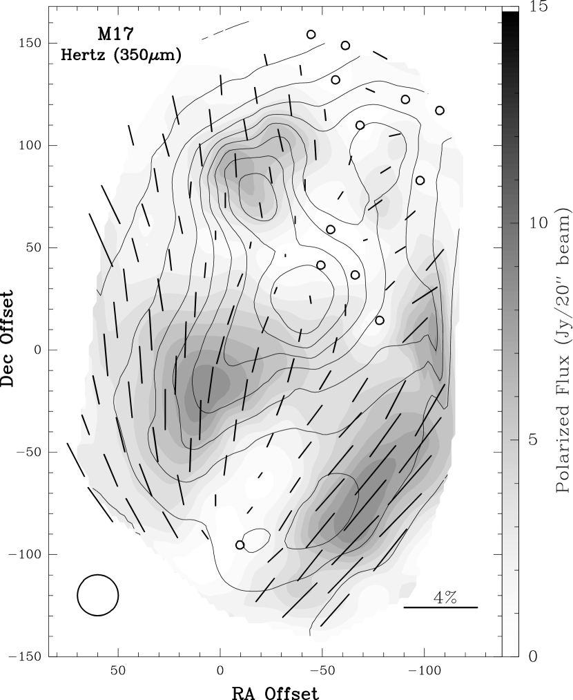
Figure 6: HERTZ Polarization map of M17 at 350 $\mu$m. All the polarization vectors shown have a polarization level and error such that $P>3\sigma_{P}$. Circles indicate cases where $P+2\sigma_{P}<1\%$. The contours delineate the total continuum flux (from 10% to 90% with a maximum flux of $\approx 700$ Jy) whereas the underlying gray scale gives the polarized flux according to the scale on the right. The beam width ($\simeq 20\arcsec$) is shown in the lower left corner and the origin of the map is at RA = $18^{\mathrm{h}}17^{\mathrm{m}}31\fs 4$, Dec = $-16\arcdeg 14\arcmin 25\farcs 0$ (B1950).

An extensive 350 $\mu$m polarimetry map of the M17 molecular cloud was obtained using the HERTZ polarimeter (Dowell et al., 1998) at the CSO on 1997 April 20 through 27 and 2001 July 19 and is presented in Figure 6. Beside the total flux (in contours) and polarized flux (in gray scale), this figure gives a detailed view (with a beam size of $\simeq 20\arcsec$) of the polarization vectors (or E vectors) across an area of more than $3\arcmin$ by $4\arcmin$. All the polarization vectors shown have a polarization level and error such that $P>3\sigma_{P}$. Circles indicate cases where $P+2\sigma_{P}<1\%$. Overall, the appearance of this map is in good qualitative agreement with results obtained at 60 $\mu$m and 100 $\mu$m by Dotson et al. (2000). Detail of the data presented in Figure 6 can be found in Table 2.

As can be seen, both the magnitude and the orientation of the polarization vectors are “well-behaved” across the map in that, at this spatial resolution, the variations are smooth and happen on a relatively large scale. The amount of polarization is seen to vary from $\approx 0\%$ to a maximum of $\approx 4\%$ which is consistent with the bulk of observations made on other objects at this wavelength. Another feature that can easily be detected, and which has important ramifications for our study, is the depolarization effect discussed earlier. A visual inspection will convince the reader that regions of higher total flux have, in general, a significantly lower level of polarization associated to them. This will be made even clearer with the help of Figure 7 where we have plotted the polarization level against the total continuum flux at $350\,\mu$m. As can be seen, there is an unmistakable anti-correlation between the two parameters with a significant reduction in the polarization levels for fluxes greater than approximately 250 Jy. This result is reminiscent of that published by Dotson (1996, see her Figure 6) for the polarization level as a function of the optical depth at 100 $\mu$m for the same object.

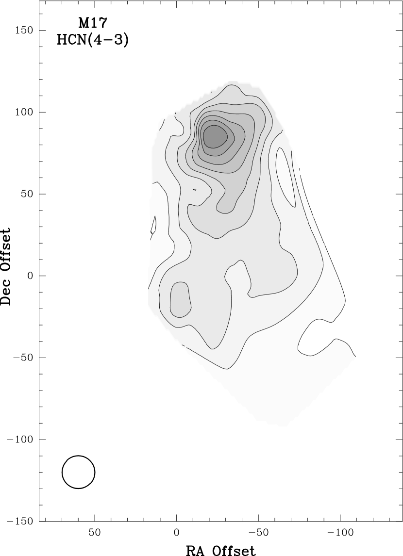
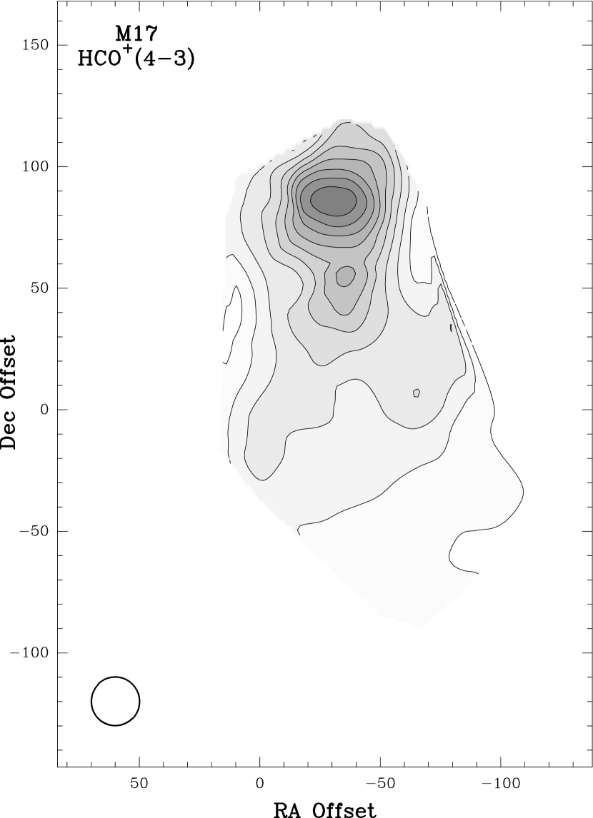
Figure 8: HCN and HCO⁺ ($J\rightarrow 4-3$) maps of M17. The lowest contour level has 12 K$\cdot$km/s and the following levels increase linearly with an interval of also 12 K$\cdot$km/s. The grid spacing of $\approx 20\arcsec$ is approximately the same size as the beam width (shown in the lower left corners) and the origin of the maps is at RA = $18^{\mathrm{h}}17^{\mathrm{m}}31\fs 4$, Dec = $-16\arcdeg 14\arcmin 25\farcs 0$ (B1950).

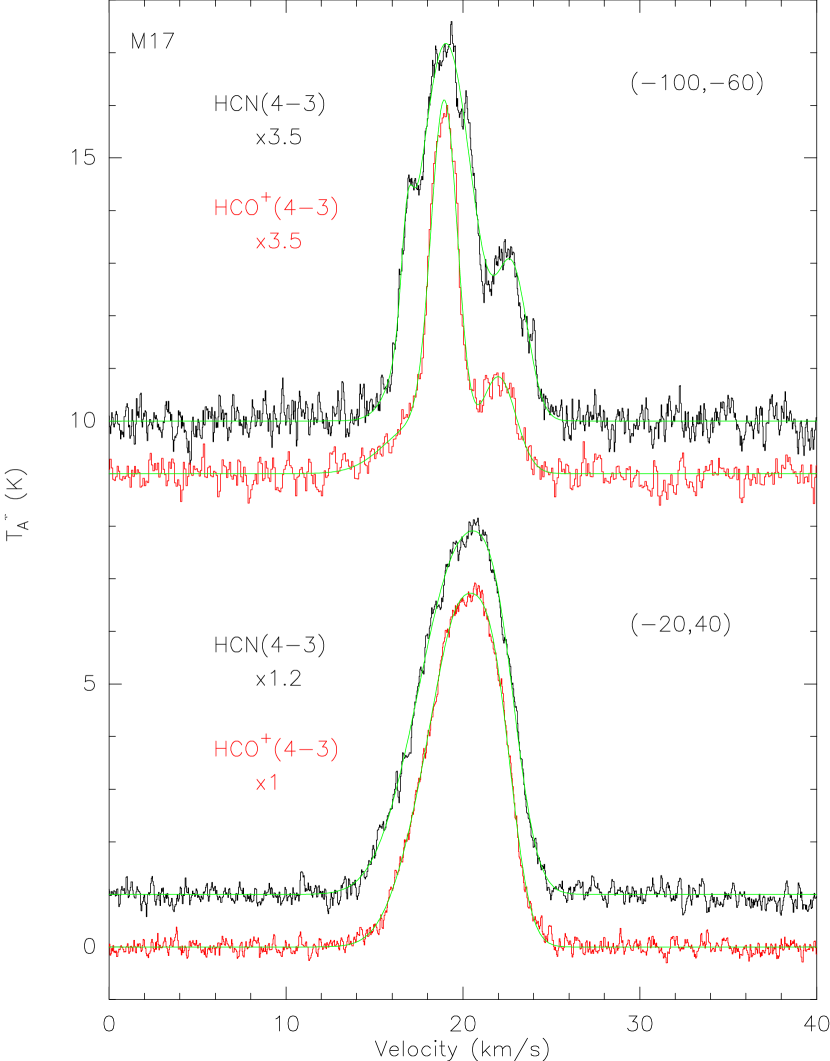
Figure 9: HCN and HCO⁺ spectra of M17 at two different positions along with a fit to their line profile. The positions are shown in parenthesis on the right side of the spectra and are relative to RA = $18^{\mathrm{h}}17^{\mathrm{m}}31\fs 4$, Dec = $-16\arcdeg 14\arcmin 25\farcs 0$ (B1950).

We present in Figure 8 HCN and HCO⁺ maps of M17 in the $J\rightarrow 4-3$ transition made at the CSO, using the facility’s 300-400 GHz receiver, during a large number of nights in the months of March, May, June and August 2001. As can be seen, the two maps have a similar appearance and are also not unlike the 350 $\mu$m continuum map presented in Figure 6. The beam size for these sets of observations is similar to the HERTZ beam at $\approx 20\arcsec$. This is a nice feature as our analysis will rest on comparisons of polarimetry and spectroscopic data across the molecular cloud. We also show in Figure 9 typical cases of spectra obtained and that were used to build these maps, along with a fit to their line profile. We can see the level of signal-to-noise ratio needed to accurately fit the line profile (and their wings) and measure the line width ratio defined earlier (which uses the variance of the lines). Each spectrum used in this study required a minimum of 8 to 10 minutes of integration (ON source) and often much more.

4.1 The line width ratio and the polarization level

We are now in a position to test the model presented in section 3 and the relationship it predicts between the ion-to-neutral line width ratio and the polarization level in molecular clouds.

We have, therefore, measured the widths $\sigma_{l,i}$ and $\sigma_{l,n}$ at every position of our M17 maps and plotted the HCO⁺/HCN line width ratio against the polarization level. This is shown in Figure 10. Whenever the spectroscopic datum was not coincident in space with any of the polarimetry data, we have used a simple bilinear interpolation technique to determine the corresponding polarization level. Referring back to the spectra shown in Figure 9, we see that the line profiles can sometimes be complicated. We modeled each line with a multi-Gaussian profile and used it in its entirety to calculate $\sigma_{l,i}$ and $\sigma_{l,n}$; i.e., we have not chosen a particular velocity component when more than one were apparent, but used the whole fit to the line shape. This is consistent with the material presented in section 2 (and in Houde et al. (2000a, b)) since the method used when comparing molecular ion and neutral lines presupposes a large number of flows (and/or velocity components). It is also more consistent with the type of comparison made here between spectroscopic and polarimetry data since it is not possible to discriminate between velocity components in the latter.

In Figure 10, we have used the normalized polarization level $P/P_{max}$ with the maximum level of polarization set at $P_{max}=7\%$. As was explained in section 3.1, this is necessary for the comparison of the line ratio to the polarimetry data. Our choice of $P_{max}$ was not done arbitrarily or neither was its value determined so as to provide a fit to the data. We have based its value on the extensive polarimetry data already obtained with HERTZ where we found that the highest levels of polarization detected so far at 350 $\mu$m were in the neighborhood of 7%. We assume that this applies well to M17 and that it corresponds to the hypothetical case where the magnetic field lies in the plane of the sky ($\alpha=\pi/2$) at a position unaffected by the depolarization effect. It should be noted that small variations in this parameter would not significantly change our results. Accompanying the data is a curve for a configuration of neutral flows with a collimation angle $\Delta\theta=34.5^{\circ}$ similar to the models defined in section 3 and presented in Figure 5, resulting from a non-linear fit to the points that delineates the “outer” limit of the data in Figure 10. The rest of the data falls neatly in the shaded area and is seen to be significantly affected by the depolarization effect discussed earlier.

While taking another look at Figure 7 for the polarization level as a function of the total flux, it should not be surprising that the clear majority of data points in Figure 10 do not take part in determining the curve that defines the collimation model. Indeed, most of them belong to regions where the flux is relatively strong and will, most likely, show a reduction in their respective polarization level. We should, therefore, expect that only a limited number of points would partake in the determination of the collimation model. An extension of the map to fainter regions of the molecular clouds could possibly alleviate this issue along with bringing an increase in the number of vectors exhibiting higher polarization levels. This would be desirable since, admittedly, our map of M17 shows no points with a polarization level greater than 4% which would allow for a better determination of the proper configuration of neutral flows and a more stringent test to our technique. Still, the outcome is encouraging and the results presented in Figure 10 are consistent with what was predicted by our model.

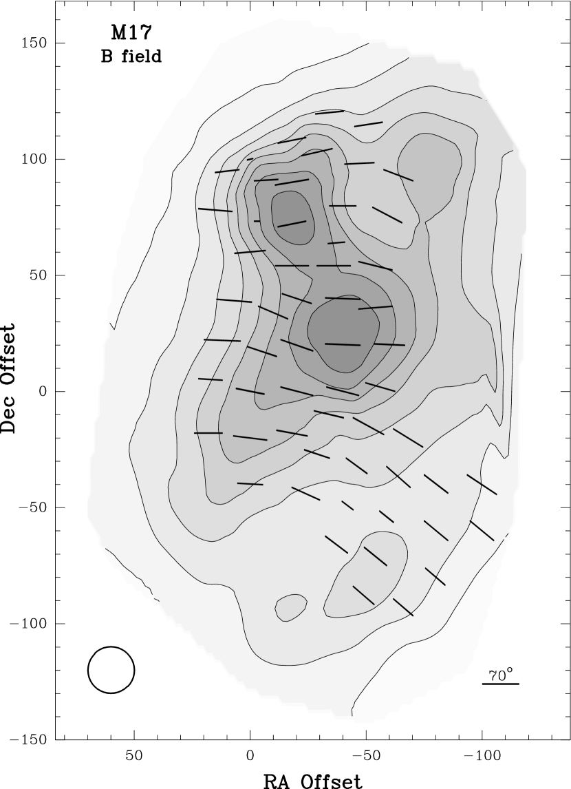
Figure 11: Orientation of the magnetic field in M17. The orientation of the projection of the magnetic field in the plane of the sky is shown by the vectors and the viewing angle is given by the length of the vectors (using the scale shown in the bottom right corner). The contours and the grey scale delineate the total continuum flux. The beam width ($\simeq 20\arcsec$) is shown in the lower left corner and the origin of the map is at RA = $18^{\mathrm{h}}17^{\mathrm{m}}31\fs 4$, Dec = $-16\arcdeg 14\arcmin 25\farcs 0$ (B1950).

We show in Figure 11 a map of the orientation of the magnetic field in M17 at every observed position. The angle $\beta$, made by the projection of the magnetic field in the plane of the sky, was obtained from the polarimetry data by rotating the corresponding polarization angle PA by $90^{\circ}$ and is represented on the map by the orientation of the vectors. The viewing angle $\alpha$, or the angle made by the magnetic field to the line of sight, was obtained by using the fit discussed above and by inverting equation (11) with the HCO⁺/HCN line width ratio as input and can be read on the map by the length of the vectors (using the scale in the bottom right). Both angles are plotted on top of the 350 $\mu$m continuum flux obtained with HERTZ.

The results are presented in more detail in Table 3. An estimate of $\sigma_{\alpha}$, the error in the viewing angle was calculated by converting the error in the HCO⁺/HCN line width ratio to that of the viewing angle through equation (11).

From Figure 11, we can observe some of the main features in the orientation of the magnetic field in M17. First, there is a gradual shift of some $40^{\circ}$ in the orientation of the projection of the magnetic field on the plane of the sky from the south-west part of the map ($\beta\sim 50^{\circ}$) to the north ($\beta\sim 90^{\circ}$). On the other hand, the viewing angle is maximum at $\alpha\sim 65^{\circ}$ in the neighborhood of the region of peak continuum emission and smoothly decreases south-westerly to a local minimum where the field is better aligned to the line of sight with $\alpha\simeq 30^{\circ}$ at RA Off $\simeq-50\arcsec$, Dec Off $\simeq-50\arcsec$. The field gradually approaches the plane of the sky, once again, in the south of the map.

Most interestingly, there is an important and localized decrease in the viewing angle of roughly $30^{\circ}-40^{\circ}$ close to the position of steepest change in continuum (or HCN and HCO⁺) emission where $\alpha$ reaches a minimum at approximately $10^{\circ}$. This region, located at RA Off $\simeq 0\arcsec$, Dec Off $\simeq 80\arcsec$, is also nearly coincident with the locations of H₂O and OH masers and the ultracompact HII region of the Northern Condensation, where Brogan & Troland (2001, see their Figure 16) have obtained a value of $B_{los}\simeq-300\,\mu$G using OH measurements at 20 km/s.

It is important to realize that $\alpha$ does not provide us with the information concerning the direction of the magnetic field relative to the plane of the sky (i.e., is it going in or coming out of the plane?), this will be provided by Zeeman measurements. We know that for M17 the magnetic field is actually coming out of the plane of the sky (Brogan & Troland, 2001, using their HI or OH Zeeman measurements at 20 km/s). The values of $\alpha$ thus obtained here are therefore relative to an axis directed toward the observer. Finally, taking into account that the magnetic field can be directed away from the line of sight by as much as $60^{\circ}$ in some parts of M17, we can see that a multiplicative factor of the order of 2 has to be applied to the Zeeman measurements of Brogan & Troland (2001) in order to evaluate the magnitude of the magnetic field. They obtained a maximum value of $\approx-750\,\mu$G for $B_{los}$, using HI Zeeman measurements at 20 km/s, implying that the magnitude of the field could be as high as $\approx 1.5$ mG for this object.

5 Discussion

In the previous sections, we have proposed a new technique, based on the work of Houde et al. (2000a, b), for evaluating the orientation of the magnetic field in molecular clouds. The orientation of the field is specified by its inclination or viewing angle $\alpha$ (see section 3.2 for a precision concerning its definition) and the angle $\beta$ made by its projection on the plane of the sky. Once determined, these parameters can also be used in conjunction with Zeeman measurements to obtain maps of the magnitude of the magnetic field. We applied this technique to spectroscopic and polarimetry data of M17 obtained at the CSO and found the results to be in good agreement with our predictions. However, as pleasing as this outcome may be, our treatment of the data rests on a number assumptions that need to be addressed and discussed.

1. At the heart of our technique is the extensive comparison of polarimetry data measured from continuum dust emission at 350 $\mu$m and line profiles of the HCN and HCO⁺ molecular species. It is, however, likely that the dust is optically thin at 350 $\mu$m whereas this is probably not true everywhere in M17 for the HCN and HCO⁺ transitions used in this study. This implies that we are, perhaps, not probing the same regions with both sets of observations, this is more likely to be true in the region of maximum HCN and HCO⁺ intensity. It is then probable that some errors are introduced in our analysis for that part of the cloud. Unfortunately, it is not possible, at this point, to say to what extent this is so. It might, therefore, be desirable to study this region of the cloud with species that are less abundant (as long as the pair of molecules used can be shown to be coexistent). Future studies using H¹³CN and H¹³CO⁺ might shed some light on this issue.

2. In the same vein, it is also not certain that given sets of spectrometric (or polarimetry) and Zeeman data would always probe the same region of a molecular cloud. As far as a comparison with the HCN and HCO⁺ is concerned, Zeeman measurements made with the CN molecular species are likely to be a better match than others made with HI or OH.

3. Again related to point 1 above is the fact that the line profiles from HCN and HCO⁺ are probably saturated in some regions of the molecular cloud. It is then likely that the line width ratio is, to some extent, subject to errors due to the different enhancement of the high velocity wings between both species. Using a pair of less abundant molecular species would also help in improving on this.

4. Small changes in the evaluation of the line width ratio can be important in determining both the appropriate neutral flow configuration to a set of data and ultimately the viewing angle. This puts stringent requirements on the modeling of the line profiles. It is extremely important that the high velocity wings be well fitted. As this is often difficult to do for a finite signal-to-noise ratio, this is likely to be a source of error in the analysis. We did our best to minimize this and we feel confident about the quality of our modeling of the line profiles, but we cannot be entirely certain that this source of error has no impact on our results.

5. Contrary to what was assumed in our analysis, it is very likely that a single model of neutral flow configuration does not apply equally well to the different regions of the molecular cloud. It is probably better to think of the chosen model as some sort of picture representative of the object under study (it tells us the maximum amount of flow collimation expected in the area covered by the observations). This is certainly another source of errors. But unlike the others discussed previously, it is possible to get a glimpse as to how severe it is likely to be. To this end, we have purposely chosen a “bad” fit to our data and calculated a new set of viewing angles and compared it with the one presented in Table 3. We show in Figure 12 histograms for the distribution of the viewing angle for the “good” (top, with $\Delta\theta=34.5^{\circ}$) and the “bad” fit where we have arbitrarily chosen a neutral flow configuration model of $\Delta\theta=60^{\circ}$ (bottom). (Alternatively, the model with $\Delta\theta=60^{\circ}$ would be a good fit to the data if $P_{max}$ were raised to approximately 15%.) As can be seen, there is a definite change in the distribution from one model to the other as the mean for the viewing angle changes from $54^{\circ}$ for the good fit to $38^{\circ}$ for the other. But, as can also be seen from a comparison of the histograms, the error occasioned by a bad selection of the neutral flow model is not likely to be much more than roughly $15^{\circ}$ to $20^{\circ}$ in the cases where $\alpha$ is measured to be high whereas it is fairly negligible when it is small. Our technique is, therefore, relatively robust to this kind of error.

6. Finally, as mentioned in the last section, M17 is lacking some higher polarization points that would allow to test our technique further out in polarization space.

In view of all this, it is important that tests be conducted on more objects to ensure the validity of the method. More precisely, we need to conduct similar studies on molecular clouds exhibiting higher levels of polarization and if possible use other less abundant species (e.g., H¹³CN and H¹³CO⁺) to better match the continuum measurements. Although such programs require a significant amount of observing time, the expected benefits are such that we judge it to be imperative to push them forward. We list here some of the most obvious benefits.

1. As was mentioned earlier, combining the kind of study presented here with Zeeman measurements (subjected to point 2 above), it is now possible to make maps for the magnitude and orientation of the magnetic field in molecular clouds.

2. It might also be possible to determine the topology of the magnetic field in molecular clouds and, perhaps, test the predictions made by different models (e.g., the helical field model of Fiege & Pudritz (2000a, b)).

3. As was hinted to in the previous section, a study of the variations in the orientation of the magnetic field through angles $\alpha$ and $\beta$ in correlation to density or density gradients might help in revealing some of the interactions between the magnetic field and its environment (e.g., field pinching during collapse).

4. The knowledge of the curve relating the ion-to-neutral line width ratio and the normalized polarization (as in Figure 10) would allow for a “correction” of the polarization levels across the source and possibly help in understanding the processes responsible for the depolarization effect observed in molecular clouds (e.g., differentiate between different grain models).

Time will tell how well our proposed technique fares and how much it can reveal concerning the nature of the magnetic field in molecular clouds. But we might be justified in being optimistic about a method that purposely uses three seemingly different and independent observational techniques and combines them in a way that takes advantage of and clearly exhibits their complementarity.

Table 1: Ion-to-neutral line width ratios in star-forming regions.

	Coordinates (1950)		$v$	$\langle$ratio$\rangle$
Source	RA	DEC	(km/s)	thick	thin
W3 IRS 5	$2^{\mathrm{h}}21^{\mathrm{m}}53\fs 3$	$61\arcdeg 52\arcmin 21\farcs 4$	$-38.1$	0.43	0.39
GL 490	$3^{\mathrm{h}}23^{\mathrm{m}}38\fs 8$	$58\arcdeg 36\arcmin 39\farcs 0$	$-13.4$	0.61	0.69
HH 7-11	$3^{\mathrm{h}}25^{\mathrm{m}}58\fs 2$	$31\arcdeg 05\arcmin 46\farcs 0$	$8.4$	1.02	$\cdots$
NGC 1333 IRAS 4	$3^{\mathrm{h}}26^{\mathrm{m}}05\fs 0$	$31\arcdeg 03\arcmin 13\farcs 1$	$8.4$	0.32	$\cdots$
L1551 IRS 5	$4^{\mathrm{h}}28^{\mathrm{m}}40\fs 2$	$18\arcdeg 01\arcmin 41\farcs 0$	6.3	0.89	$\cdots$
OMC-1	$5^{\mathrm{h}}32^{\mathrm{m}}47\fs 2$	$-05\arcdeg 24\arcmin 25\farcs 3$	9.0	0.55	0.22
OMC-3 MMS 6	$5^{\mathrm{h}}32^{\mathrm{m}}55\fs 6$	$-05\arcdeg 03\arcmin 25\farcs 0$	11.3	0.51	0.48
OMC-2 FIR 4	$5^{\mathrm{h}}32^{\mathrm{m}}59\fs 0$	$-05\arcdeg 11\arcmin 54\farcs 0$	11.2	0.76	0.27
L1641N	$5^{\mathrm{h}}33^{\mathrm{m}}52\fs 5$	$-06\arcdeg 24\arcmin 00\farcs 0$	7.5	0.65	$\cdots$
NGC 2024 FIR 5	$5^{\mathrm{h}}39^{\mathrm{m}}12\fs 7$	$-01\arcdeg 57\arcmin 03\farcs 3$	11.5	0.95	$\cdots$
NGC 2071	$5^{\mathrm{h}}44^{\mathrm{m}}30\fs 2$	$00\arcdeg 20\arcmin 42\farcs 0$	9.5	0.93	0.64
Mon R2	$6^{\mathrm{h}}05^{\mathrm{m}}20\fs 3$	$-06\arcdeg 22\arcmin 47\farcs 0$	10.5	1.03	$\cdots$
GGD 12	$6^{\mathrm{h}}08^{\mathrm{m}}23\fs 9$	$-06\arcdeg 11\arcmin 04\farcs 0$	10.9	0.78	$\cdots$
S269	$6^{\mathrm{h}}11^{\mathrm{m}}46\fs 4$	$13\arcdeg 50\arcmin 33\farcs 0$	19.2	0.69	$\cdots$
AFGL961E	$6^{\mathrm{h}}31^{\mathrm{m}}59\fs 1$	$04\arcdeg 15\arcmin 09\farcs 0$	13.7	0.95	$\cdots$
NGC 2264	$6^{\mathrm{h}}38^{\mathrm{m}}25\fs 6$	$09\arcdeg 32\arcmin 19\farcs 0$	8.2	0.85	0.88
M17 SWN	$18^{\mathrm{h}}17^{\mathrm{m}}29\fs 8$	$-16\arcdeg 12\arcmin 55\farcs 0$	19.6	0.90	0.81
M17 SWS	$18^{\mathrm{h}}17^{\mathrm{m}}31\fs 8$	$-16\arcdeg 15\arcmin 05\farcs 0$	19.7	0.90	0.78
DR 21(OH)	$20^{\mathrm{h}}37^{\mathrm{m}}13\fs 0$	$42\arcdeg 12\arcmin 00\farcs 0$	$-2.6$	0.80	0.69
DR 21	$20^{\mathrm{h}}37^{\mathrm{m}}14\fs 5$	$42\arcdeg 09\arcmin 00\farcs 0$	$-2.7$	0.98	0.58
S140	$22^{\mathrm{h}}17^{\mathrm{m}}40\fs 0$	$63\arcdeg 03\arcmin 30\farcs 0$	$-7.0$	0.80	0.85

Table 2: M17 350 µm Results

$\Delta\alpha$	$\Delta\delta$	P	$\sigma_{\rm{P}}$	PA	$\sigma_{\rm{PA}}$	Flux
-120	95	0.84	0.57	151.9	19.5	255.7
-115	-51	3.62	1.55	148.7	12.2	151.0
-115	78	0.76	0.61	112.9	22.8	249.6
-110	-69	3.61	1.60	149.9	12.7	127.6
-110	61	0.82	0.45	135.0	15.7	255.3
-108	117	0.16	0.34	42.6	60.5	297.6
-105	-86	1.74	1.77	133.7	29.4	106.5
-105	44	1.47	0.41	140.1	8.0	284.0
-103	-29	3.21	0.96	149.9	8.5	206.3
-103	100	0.64	0.28	145.9	12.4	310.3
-100	-103	0.60	1.60	91.6	76.3	94.3
-100	27	1.62	0.42	123.3	7.4	368.4
-98	-47	3.78	0.39	143.0	2.9	214.3
-98	83	0.52	0.22	124.2	12.0	326.3
-95	-120	5.36	16.45	121.4	87.9	71.1
-95	10	1.87	0.46	134.1	7.1	374.2
-95	139	0.95	0.76	176.0	23.1	240.4
-93	-64	3.62	0.29	139.3	2.3	206.0
-93	66	0.76	0.20	128.3	7.6	348.3
-91	122	0.35	0.13	69.5	10.7	315.3
-90	-7	1.48	0.52	134.6	10.2	309.6
-88	-81	3.30	0.34	135.8	2.9	171.9
-88	49	0.61	0.18	122.8	8.5	371.1
-86	-25	2.36	0.25	152.5	3.0	264.2
-86	105	0.62	0.06	98.3	2.7	444.9
-83	-98	2.91	0.37	142.2	3.6	151.1
-83	32	0.64	0.15	139.0	6.8	413.1
-81	-42	2.87	0.18	143.5	1.7	252.4
-81	88	0.64	0.05	119.9	2.3	475.5
-78	-115	1.67	0.56	140.7	9.6	116.5
-78	15	0.44	0.24	166.8	15.7	407.4
-78	144	0.87	0.19	60.7	6.2	233.1
-76	-59	3.50	0.16	140.8	1.3	261.6
-76	71	0.92	0.06	128.6	1.8	426.4
-73	-132	0.92	1.62	131.2	50.9	105.7
-73	-3	0.94	0.62	157.0	18.5	365.0
-73	127	0.46	0.07	66.3	4.5	304.9
-71	-76	3.56	0.16	141.1	1.2	269.9
-71	54	0.23	0.07	123.4	10.8	452.8
-69	110	0.12	0.05	63.8	11.8	416.9
-68	-20	1.48	0.10	147.7	1.9	317.6
-66	-93	3.73	0.17	136.9	1.3	238.0
-66	37	0.26	0.09	11.6	9.6	533.1
-64	-37	1.84	0.11	138.6	1.6	283.5
-64	93	0.47	0.05	161.5	3.1	424.7
-61	-110	2.76	0.32	136.5	3.4	151.6
-61	20	0.65	0.07	177.0	3.1	567.3
-61	149	0.48	0.20	88.9	12.2	169.0
-59	-54	2.08	0.11	140.1	1.5	275.5
-59	76	0.45	0.05	151.3	3.1	368.7
-56	-127	2.36	0.58	139.5	7.0	130.7
-56	2	0.87	0.10	164.5	2.5	485.7
-56	132	0.22	0.09	42.9	11.9	235.3
-54	-71	2.35	0.10	139.2	1.3	305.4
-54	59	0.07	0.06	149.4	18.5	477.3
-51	-144	0.68	1.49	178.9	62.1	135.5
-51	-15	1.14	0.06	151.0	1.4	377.6
-51	115	0.67	0.06	7.5	2.8	312.8
-49	-88	2.46	0.12	140.7	1.4	317.5
-49	42	0.19	0.07	4.8	11.8	625.6
-47	98	1.06	0.05	2.6	1.3	398.6
-46	-32	1.35	0.07	143.0	2.0	313.7
-44	-105	2.13	0.17	141.6	2.3	236.2
-44	24	0.41	0.03	7.7	3.8	710.6
-44	154	0.39	0.30	100.1	22.2	111.7
-42	-49	1.16	0.08	143.2	2.1	258.9
-42	81	0.60	0.04	179.1	2.0	419.0
-39	-122	2.71	0.38	134.0	4.0	171.3
-39	7	0.72	0.05	168.1	2.5	631.8
-39	137	0.52	0.13	5.4	7.1	175.9
-37	-66	1.01	0.08	143.5	2.4	247.7
-37	64	0.38	0.03	2.3	2.5	559.4
-34	-139	0.70	1.83	60.7	75.3	148.9
-34	-10	1.35	0.08	165.7	1.3	416.1
-34	120	1.11	0.07	6.1	1.8	298.4
-32	-83	1.26	0.09	148.9	2.1	276.6
-32	46	0.12	0.03	171.8	10.6	584.6
-29	-27	1.15	0.08	159.0	1.8	344.0
-29	103	1.28	0.03	11.7	0.7	507.3
-27	-100	1.11	0.16	131.8	4.2	273.1
-27	29	0.37	0.03	157.3	2.6	654.5
-27	159	0.45	0.43	65.3	27.1	86.0
-25	86	0.87	0.03	9.4	0.9	625.5
-24	-44	0.81	0.06	153.8	2.1	271.3
-22	-117	1.68	0.45	140.8	7.7	213.5
-22	12	0.93	0.04	161.1	1.1	579.3
-22	142	0.66	0.17	12.6	7.3	131.6
-20	-61	0.34	0.07	156.3	5.7	243.7
-20	68	0.80	0.03	11.5	1.0	677.0
-17	-5	1.42	0.03	167.1	0.7	496.5
-17	125	0.91	0.10	7.9	3.2	200.8
-15	-78	0.48	0.08	143.2	4.7	253.8
-15	51	0.39	0.03	174.3	3.7	525.4
-12	-22	1.71	0.04	171.4	0.6	431.0
-12	108	1.18	0.04	7.4	1.0	352.4
-10	-95	0.31	0.12	130.8	10.7	279.3
-10	34	0.71	0.04	156.9	1.6	476.5
-10	164	0.86	0.82	68.7	27.3	58.8
-7	-39	1.17	0.05	174.5	1.2	340.5
-7	90	1.31	0.03	4.8	0.6	589.0
-5	-112	0.62	0.27	123.5	12.5	220.6
-5	17	1.08	0.03	162.1	0.8	483.6
-5	147	0.54	0.39	173.6	20.8	100.9
-3	73	0.83	0.03	177.8	1.2	545.4
-2	-56	1.09	0.06	173.4	1.7	268.8
0	-130	1.83	1.35	114.8	21.1	165.4
0	0	1.56	0.03	167.3	0.6	490.0
0	130	1.02	0.14	4.4	4.0	141.8
2	56	0.49	0.05	6.6	2.9	377.4
3	-73	0.63	0.07	2.3	3.3	226.9
5	-17	2.01	0.03	173.2	0.5	471.7
5	112	1.22	0.09	7.5	2.2	196.4
7	-90	0.58	0.12	31.8	6.0	206.3
7	39	0.79	0.10	175.4	2.3	329.1
10	-34	2.13	0.05	177.1	0.6	409.9
10	95	1.18	0.05	5.6	1.3	313.1
12	-108	0.32	0.48	101.5	42.8	169.3
12	22	1.36	0.05	177.3	1.1	324.0
12	152	0.51	0.77	79.2	43.7	67.9
15	-51	1.83	0.05	178.6	0.8	343.7
15	78	0.88	0.06	176.8	2.1	293.8
17	5	1.97	0.04	177.7	0.6	352.2
17	134	1.16	0.52	20.8	12.9	105.3
20	-68	1.66	0.07	12.4	1.3	265.8
20	61	1.00	0.12	14.6	3.4	226.9
22	-12	2.13	0.05	178.7	0.7	362.3
22	117	1.60	0.24	12.4	4.3	132.8
24	44	1.11	0.11	6.6	2.8	224.7
25	-86	1.67	0.20	30.9	3.4	195.0
27	-29	2.24	0.05	180.0	0.6	308.3
27	100	1.30	0.13	14.8	2.8	149.7
29	27	1.75	0.08	7.9	1.3	223.2
32	-46	1.91	0.06	6.7	0.9	298.4
32	83	1.35	0.25	9.2	5.4	157.3
34	10	2.20	0.08	5.0	1.0	240.9
37	-64	1.92	0.12	21.2	1.8	226.8
37	66	1.23	0.20	17.2	4.6	156.5
39	-7	2.05	0.07	3.0	1.0	238.2
42	-81	2.06	0.22	29.9	3.1	156.4
42	49	1.28	0.17	15.0	3.9	159.5
44	-24	1.99	0.09	5.9	1.2	232.0
44	105	1.10	0.36	14.6	9.5	112.8
46	32	1.73	0.26	6.7	4.2	168.5
49	-42	1.92	0.10	14.1	1.4	209.9
51	15	2.03	0.20	7.3	2.9	178.1
54	-59	1.87	0.13	22.5	2.0	168.2
54	71	2.33	0.42	24.5	5.1	114.4
56	-2	2.28	0.14	4.5	1.7	180.2
59	-76	2.32	0.30	35.1	3.7	130.7
59	54	3.17	0.48	24.3	4.3	118.0
61	-20	1.54	0.14	13.1	2.6	195.2
66	-37	1.17	0.14	22.2	3.4	198.9
71	-54	2.02	0.25	27.8	3.5	163.1

Table 3: M17 - Magnetic Field Orientation

$\Delta\alpha$	$\Delta\delta$	$\alpha$	$\sigma_{\alpha}$	$\beta$	$\sigma_{\beta}$
-100	-60	59.9	5.5	52.6	5.5
-100	-40	68.8	0.3	55.3	5.1
-80	-80	51.8	1.4	48.8	1.2
-80	-60	61.0	0.4	50.5	1.1
-80	-40	60.2	0.5	53.9	1.7
-68	-20	67.8	0.3	57.5	1.3
-66	-93	51.8	2.5	46.9	1.3
-64	-37	62.6	1.1	48.8	0.8
-64	93	60.7	0.3	70.8	3.0
-60	20	61.7	0.1	87.6	1.6
-59	-54	37.7	8.7	50.1	1.4
-59	76	65.0	0.4	61.1	2.8
-56	2	59.6	0.3	74.2	2.5
-54	-71	57.9	0.9	49.2	1.1
-54	36	68.1	1.5	95.7	3.8
-54	54	67.1	0.2	75.8	18.7
-51	-15	67.2	0.9	61.1	1.3
-51	115	57.7	0.6	97.4	1.5
-49	-88	55.7	2.1	50.7	1.0
-47	98	58.5	0.9	92.5	1.1
-46	-32	52.1	0.6	53.3	2.0
-42	-49	28.4	3.3	53.0	2.1
-40	0	65.3	0.1	76.0	1.6
-40	20	67.9	0.1	86.9	1.3
-40	40	68.9	0.1	88.4	3.2
-40	80	55.4	0.2	90.9	1.8
-37	-66	57.0	0.8	53.3	2.1
-37	64	34.6	1.6	92.2	1.7
-36	54	63.8	0.1	89.5	3.2
-34	-10	62.1	0.4	75.7	1.4
-34	120	57.4	0.4	96.1	1.8
-29	-27	53.7	1.7	69.3	1.8
-29	103	63.1	2.0	101.6	0.6
-24	-44	59.7	0.5	64.6	2.0
-20	0	64.4	1.0	75.6	0.8
-20	20	66.4	0.3	70.3	1.4
-20	40	63.2	0.2	72.0	2.7
-18	-18	62.3	0.3	78.7	0.7
-18	54	67.1	0.5	90.7	1.0
-18	72	57.7	0.2	99.6	0.8
-18	90	65.2	0.1	97.5	0.6
-18	108	55.0	0.7	99.0	0.7
-10	34	64.8	2.1	67.0	1.6
-7	91	50.5	1.5	94.8	0.2
-5	17	62.9	0.9	72.1	0.7
-3	73	9.4	6.9	88.3	0.4
0	-40	50.8	1.5	86.0	0.4
0	-20	66.5	0.3	83.0	0.4
0	0	55.2	2.4	77.3	0.5
0	60	62.3	1.4	92.7	1.8
0	100	9.4	6.9	95.7	0.6
7	39	67.3	1.3	85.0	2.1
10	95	49.9	2.5	95.5	1.1
12	22	71.5	1.2	87.1	0.3
15	78	64.1	1.4	87.3	1.5
17	5	49.5	10.0	87.6	0.1
18	-18	57.7	7.0	87.3	0.5

Figure 1: Definition of the coordinate system (axes N for North, E for East and LOS for line-of-sight) and of the angles $\alpha$ and $\beta$ characterizing the spatial orientation of the magnetic field vector (thick line and arrow).

Figure 2: An example of a neutral flow configuration. The flows (thin lines and arrows) are all contained within a cone of angular width $\Delta\theta$ centered on the symmetry axis as defined by the orientation magnetic field vector (thick line and arrow).

Figure 3: The ion line width vs the neutral line width for every pair of spectra obtained for the sources presented in Table 1. HCO⁺ is plotted against HCN and H¹³CO⁺ against H¹³CN. The two straight lines correspond to the upper and lower limits discussed in the text where the line width ratio is $\simeq 1$ and $\simeq 0.26$, respectively. The cluster of open circles all pertain to spectra obtained on the same object (M17, which will be discussed later).

Figure 4: The ion-to-neutral line width ratio vs the viewing angle $\alpha$ for angles of neutral flow collimation of $20^{\circ}$, $40^{\circ}$, $60^{\circ}$ and $90^{\circ}$ (no collimation). Every curve is monotonic and has a ratio $\simeq 1$ at $\alpha=0$ and $\simeq 0.26$ at $\alpha=\pi/2$.

Figure 5: The ion-to-neutral line width ratio vs the normalized polarization level ($P/P_{max}$) for angles of neutral flow collimation of $20^{\circ}$, $40^{\circ}$, $60^{\circ}$ and $90^{\circ}$ (no collimation). Every curve is monotonic and has a ratio $\simeq 1$ at $\alpha=0$ and $\simeq 0.26$ at $\alpha=\pi/2$. The shaded part represents the region where we should expect corresponding data points to be located in cases where $\Delta\theta=90^{\circ}$ (see text).

Figure 7: Polarization level vs the total flux. Taken from the 350 $\mu$m HERTZ polarization map of M17 shown in Figure 6. The polarization levels have $P>3\sigma_{P}$ or $P+2\sigma_{P}<1\%$. The depolarization effect discussed in the text is clearly seen.

Figure 10: The HCO⁺/HCN line width ratio vs the normalized polarization level ($P/P_{max}$) for M17. $P_{max}$ is set at 7% and the data is shown against a model of neutral flow collimation of $\Delta\theta=34.5^{\circ}$. The polarization levels have $P>3\sigma_{P}$ or $P+2\sigma_{P}<1\%$.

Figure 12: Histograms showing the distribution of the viewing angle $\alpha$ in M17 for (top) our fit to the data shown in Figure 5 ($\Delta\theta=34.5^{\circ}$) and (bottom) another where $\Delta\theta=60^{\circ}$.

References

- Brogan & Troland (2001) Brogan, C. L., Troland, T. H., 2001, ApJ, 560, 821
- Brogan et al. (1999) Brogan, C. L., Troland, T. H., Roberts, D. A., Crutcher, R. M. 1999, ApJ, 515, 304
- Choudhuri (1998) Choudhuri, A. R. 1998, The Physics of Fluids and Plasmas, an Introduction for Astrophysicists (Cambridge: Cambridge), ch. 13
- Crutcher et al. (1993) Crutcher, R. M., Troland, T. H., Goodman, A. A., Heiles, C., Kaz s, I., & Myers, P. C. 1993, ApJ, 407, 175
- Crutcher et al. (1999) Crutcher, R. M., Troland, T. H., Lazareff, B., Paubert, G., Kaz s, I. 1999, ApJ, 514, L121
- Davis & Greenstein (1952) Davis, L. M. & Greenstein, J. L. 1952, ApJ, 114, 206
- Dotson et al. (2000) Dotson, J. L., Davidson, J., Dowell, C. D., Schleuning, D. A., Hildebrand, R. H. 2000, ApJS, 128, 335
- Dotson (1996) Dotson, J. L. 1996, ApJ, 470, 576
- Dowell et al. (1998) Dowell, C. D., Hildebrand, R. H., Schleuning, D. A., Vaillancourt, J. E., Dotson, J. L., Novak, G., Renbarger, T., Houde, M. 1998, ApJ, 504, 588
- Fiege & Pudritz (2000a) Fiege, J. D., Pudritz, R. E. 2000a, MNRAS, 311, 85
- Fiege & Pudritz (2000b) Fiege, J. D., Pudritz, R. E. 2000b, MNRAS, 311, 105
- Heiles (1997) Heiles, C. 1997, ApJS, 111, 245
- Hildebrand (1996) Hildebrand, R. H. 1996, in Polarimetry of the Interstellar Medium, ed. W. G. Roberge, D. C. B. Whittet (San Francisco: Astronomical Society of the Pacific), 254
- Hildebrand (1988) Hildebrand, R. H. 1988 QJRAS, 29, 327
- Houde et al. (2000a) Houde, M., Bastien, P., Peng, R., Phillips, T. G., and Yoshida, H.2000a, ApJ, 536, 857
- Houde et al. (2000b) Houde, M., Peng, R., Phillips, T. G., Bastien, P. and Yoshida, H. 2000b, ApJ, 537, 245
- Houde et al. (2001) Houde, M., Phillips, T. G., Bastien, P., Peng, R., and Yoshida, H. 2001, ApJ, 547
- Rao et al. (1998) Rao, R., Crutcher, R. M., Plambeck, R. L., and Wright, M. C. H. 1998, ApJ, 502, L75
- Weintraub, Goodman and Akeson (2000) Weintraub, D. A., Goodman, A. A., Akeson, R. L. 2000, in Protostars and Planets IV, ed. V. Mannings, A. P. Boss, S. S. Russel (Tucson: The University of Arizona Press), 247