The Globular Cluster System of NGC 5128 I. Survey and Catalogs

Abstract

We present the results of a photometric and spectroscopic survey of the globular cluster system of NGC 5128 (Centaurus A), a galaxy whose proximity makes it an important target for early-type galaxy studies. We imaged three fields in UBVRI that extend 50 and 30 kpc along the major and minor axes, respectively. We used both color and size information to develop efficient selection criteria for differentiating between star clusters and foreground stars. In total, we obtained new velocities for 138 globular clusters, nearly tripling the number of known clusters, and bringing the confirmed total in NGC 5128 to 215. We present a full catalog of all known GCs, with their positions, photometry, and velocities. In addition, we present catalogs of other objects observed, such as foreground stars, background galaxies, three Galactic white dwarfs, seven background QSOs, and 52 optical counterparts to known X-ray point sources. We also report an observation of the cluster G169, in which we confirm the existence of a bright emission line object. This object, however, is unlikely to be a planetary nebula, but may be a supernova remnant.

1. Introduction

Systems of globular clusters are a nearly ubiquitous feature of all nearby galaxies. Globular clusters (GCs), which are typically old with sub-solar metallicities, are the most visible remnants of intense star formation that occurred in a galaxy’s distant past. As single-age, single-metallicity stellar populations, GCs are ideal for studying the fossil remains of a galaxy’s star formation and metal-enrichment history.

The past decade has seen a rapid growth in the study of extragalactic GC systems. The availability of the Hubble Space Telescope (HST) in particular has enabled the study of GC systems in galaxies well beyond the Local Group. One of the more striking results of these studies is the frequency with which the metallicity distributions of these GC systems are bimodal (e.g. Larsen et al. 2001; Kundu & Whitmore 2001). Different scenarios of galaxy formation (or at least of globular cluster system formation) have been proposed or adapted to explain the observed metallicity distributions and other properties of GC systems: mergers of spiral galaxies (Ashman & Zepf 1992), multiple in situ star formation epochs (Forbes, Brodie, & Grillmair 1997), dissipationless hierarchical merging of protogalactic clumps (Côté, Marzke, & West 1998), and more generalized hierarchical merging (Beasley et al. 2002). The question that all of these scenarios address largely concerns the nature and time frame of merging or gas dissipation. Elements of all of these scenarios are supported by various studies of different facets of galaxy formation and evolution. For example, the supernova winds that some use to explain the suppression of star formation in dwarf galaxies at high redshift (Dekel & Silk 1986) has also been proposed as a possible mechanism for the truncation of metal-poor GC formation at early times (Beasley et al. 2002). Similarly, hierarchical merging models are often used to explain the mass assembly of present-day galaxies.

While most spheroid formation may have occurred in the past (at redshifts $z>2$), present-day examples of recent merger remnants may give us a window onto this distant epoch. Locally, there is compelling evidence that some ellipticals have recently interacted or merged with another galaxy. Many ellipticals possess large-scale disks of gas and dust. Faint structure in the form of loops, shells, ripples, and tails are especially visible in the outer regions of ellipticals (Malin & Carter 1983), and are presumably the aftermaths of a recent interaction. One such galaxy, and perhaps the best candidate for study, is the nearby elliptical, NGC 5128. We have chosen to examine of the stellar content of NGC 5128 in order to further elucidate its formation history and gain insight on the formation of other ellipticals. Our survey of the planetary nebula (PN) system in NGC 5128’s outer halo represents the kinematics of the field star population, and is presented in a separate paper (Peng, Ford, & Freeman 2004). In this paper, we describe our photometric and spectroscopic survey for globular clusters, and present the resulting catalogs of objects.

2. The GC system of NGC 5128

As the nearest large elliptical galaxy, and as a recent merger remnant, NGC 5128 (also known as the radio source Centaurus A) is an obvious target for GC system studies. At a distance of 3.5 Mpc (Hui et al. 1993), NGC 5128 is the only early-type member of the Centaurus group, an environment of lower density than galaxy clusters which harbor many of the luminous ellipticals previously studied. There is also much observational evidence that NGC 5128 has experienced one or more major merging events, including a warped disk of gas and dust at its center, faint shells and extensions in its light profile (Malin 1978), and a young tidal stream in its halo (Peng, Ford, Freeman, & White 2002). It is also known to have a bimodal distribution of globular cluster metallicities (Zepf & Ashman 1993; Held et al. 1997). NGC 5128 is by far the nearest active radio galaxy, and exhibits signatures of recent star formation where the radio jet has interacted with shells of H I (Graham 1998). For a recent and complete review of this galaxy, see Israel (1998). The combination of its proximity and post-merger state makes NGC 5128 an excellent target for a detailed study.

NGC 5128’s peculiar appearance and nature has long led astronomers to believe that it is somehow unique. However, as Ebneter & Balick (1983) point out in their review, the galaxy’s proximity permits us to collect data more detailed than for most other galaxies, and thus makes it seem more peculiar. In fact, NGC 5128 is rather typical member of the population of dusty elliptical galaxies and radio galaxies. Massive galaxies with old stellar populations and central dust obscuration are known to host radio sources in both the local universe and at redshifts out to and beyond $z\sim 1$ (e.g. Zirm, Dickinson, & Dey 2003).

Some of the early work on extragalactic GCs was done in NGC 5128. Noting a slightly diffuse 17th magnitude object on photographic plates, Graham & Phillips (1980; GP80) obtained follow-up spectroscopy and identified the first GC in this galaxy. Five more GCs were confirmed by van den Bergh, Hesser, & G.Harris (1981; VHH81). Using UVR star counts, G.Harris, Hesser, H.Harris, & Curry (1984) estimated that the total cluster population in NGC 5128 is 1200–1900. Subsequent spectroscopic work (Hesser, H.Harris, & G.Harris 1986 [HHH86]; Sharples 1988) increased the number of GCs with radial velocities. Finally, G.Harris et al. (1992; HGHH92) obtained CCD photometry on the Washington system for 62 confirmed GCs. This study produced one of the best GC system metallicity distributions at the time, and was later cited by Zepf & Ashman (1993) as evidence for bimodality.

Since then, the relatively small fields of view of modern detectors have forced studies to concentrated on the inner regions of the NGC 5128 GC system. Minniti et al. (1996; MAGJM96) used infrared imaging to identify possible intermediate-age, metal-rich GCs. Holland, Côté, & Hesser (1999; HCH99) used HST WFPC2 imaging to identify spatially resolved GC candidates in the region near the dust lane. Rejkuba (2001) showed what is possible with excellent (0$\farcs$6) seeing and 8-meter telescopes when she used imaging taken at the Very Large Telescope to define a sample of fainter GC candidates based on their resolved appearance in two $7\arcmin\times 7\arcmin$ fields. Only with the availability of mosaic cameras are CCD studies now able to cover an area comparable to the photographic studies of the 1980s. Recent programs include this one and an imaging study using the Big Throughput Camera on the CTIO 4-meter (G.Harris & W.Harris 2003) with the Washington photometric system (Canterna 1976).

Unfortunately, NGC 5128’s nearness and relative proximity to the Galactic bulge and disk ($l=309\fdg 5$, $b=+19.4$) conspire to make GC studies difficult. At the distance of NGC 5128, $1\arcmin=1.02$ kpc, which means that NGC 5128’s halo subtends over two degrees of sky. The density of foreground stars is also high, such that even in the central regions, all but a few percent of objects within the magnitude range expected for NGC 5128 GCs are actually stars in our own Milky Way. Spectroscopic follow-up to obtain radial velocities is the only way to confidently identify true GCs. It is only with the relatively recent development of wide-field imaging and spectroscopy that we have been able to substantially increase the sample of known GCs in NGC 5128. Despite these difficulties, the return on these investigations has the potential to be large — NGC 5128 is the only large elliptical whose stellar populations can be studied in detail, and its proximity makes it the local benchmark for studies of more distant early-type galaxies.

3. A UBVRI Broadband
Imaging Survey of NGC 5128

3.1. Observations

Table 1CTIO Mosaic UBVRI Observations

Field	RA	DEC	Field-of-View	U	B	V	R	I
	(J2000)	J2000	arcmin	(sec)	(sec)	(sec)	(sec)	(sec)
				(″)a	(″)a	(″)a	(″)a	(″)a
CTR	13:25:30	$-$43:01:33	$37.6\times 38.6$	3600	1500	1800	1000	1000
				1.20	1.27	1.25	1.24	1.18
NE	13:26:46	$-$42:28:25	$36.0\times 38.1$	$3719^{b}$	1500	1800	1800	1500
				1.38	1.32	1.21	1.04	1.26
S	13:25:27	$-$43:26:30	$37.2\times 39.1$	$3662^{b}$	1500	1800	1800	$1608^{b}$
				1.26	1.12	0.96	1.11	1.97

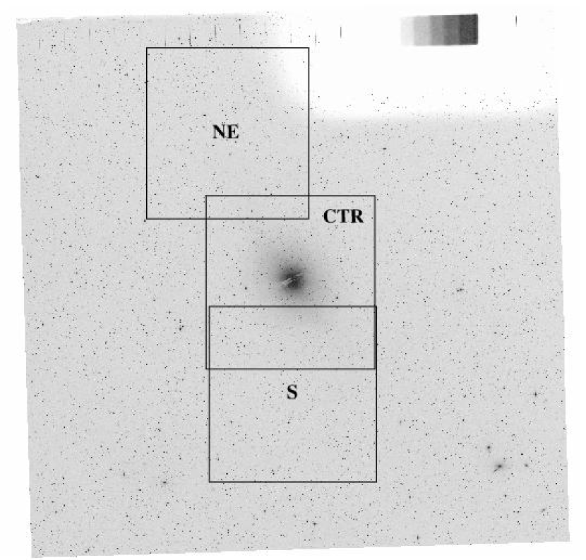
Figure 1.— Our three Mosaic II fields overplotted on a $2\arcdeg\times 2\arcdeg$ Digitized Sky Survey image of NGC 5128. North is up and East is to the left. Fields are referred to in the text by the positions relative to the galaxy: CTR, NE, and S. The exact centers and dimensions of each field is presented in Table 1.

We conducted our imaging survey with the Mosaic II optical CCD camera on the Blanco 4-meter telescope at Cerro Tololo Inter-American observatory (CTIO). We observed three fields with Mosaic II, which has $0\farcs 26$ pixels and a 0$\fdg$5 field-of-view. We imaged through the Johnson-Cousins UBVRI filters on the nights of 1–3 June 2000. These 38′$\times$38′ dithered fields are shown in Figure 1. The center field (CTR) is centered on the galaxy. The northeast (NE) field was chosen to follow the faint halo light out along the major axis, while the south (S) field was chosen to avoid galactic cirrus and observe a large “sky” area, as determined from Malin’s deep photographic image (Malin 1978). The V-band image of each field is shown in Figures 2, 3, and 4. The total exposure times in UBVRI were 3600s, 1500s, 1800s, 1000s, and 1000s, respectively, for the CTR field. For the other two fields, we went slightly deeper in U,R, and I with exposure times of 3900s, 1500s, 1800s, 1800s, and 1500s, respectively. We split our observations in each band into a series of five dithered exposures (six for U and I in the NE and S fields). Conditions were non-photometric on the first night, but were photometric for the remainder of the observing run. All images taken on the first night were calibrated by images taken on the subsequent nights. The seeing had a range of 1″–2″, with a median value of $1\farcs 24$. For the image sets with some non-photometric data, we calculate the “effective” exposure time, which is the equivalent exposure time that would be necessary during photometric conditions to reach the same flux levels we measure in our images. This information is summarized in Table 1.

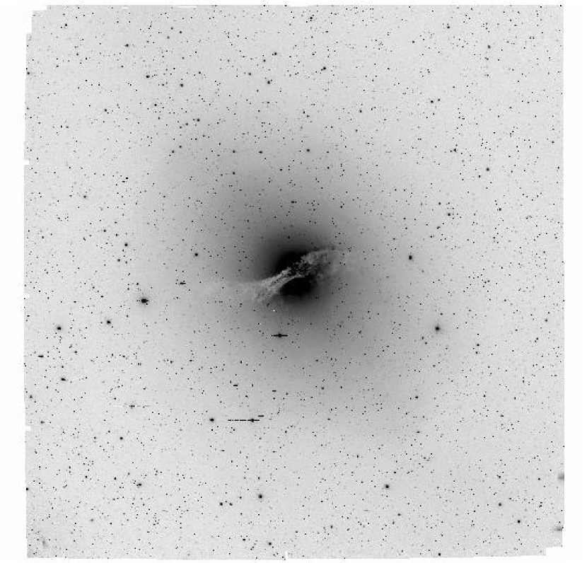
Figure 2.— V-band image of the CTR field. North is up, East is to the left.

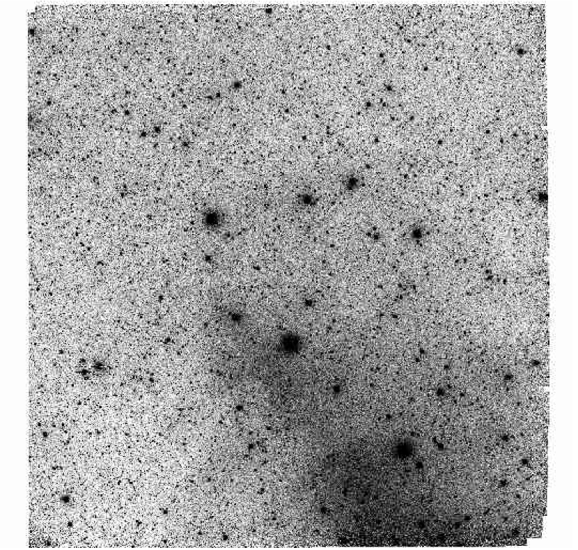
Figure 3.— V-band image of the NE field.

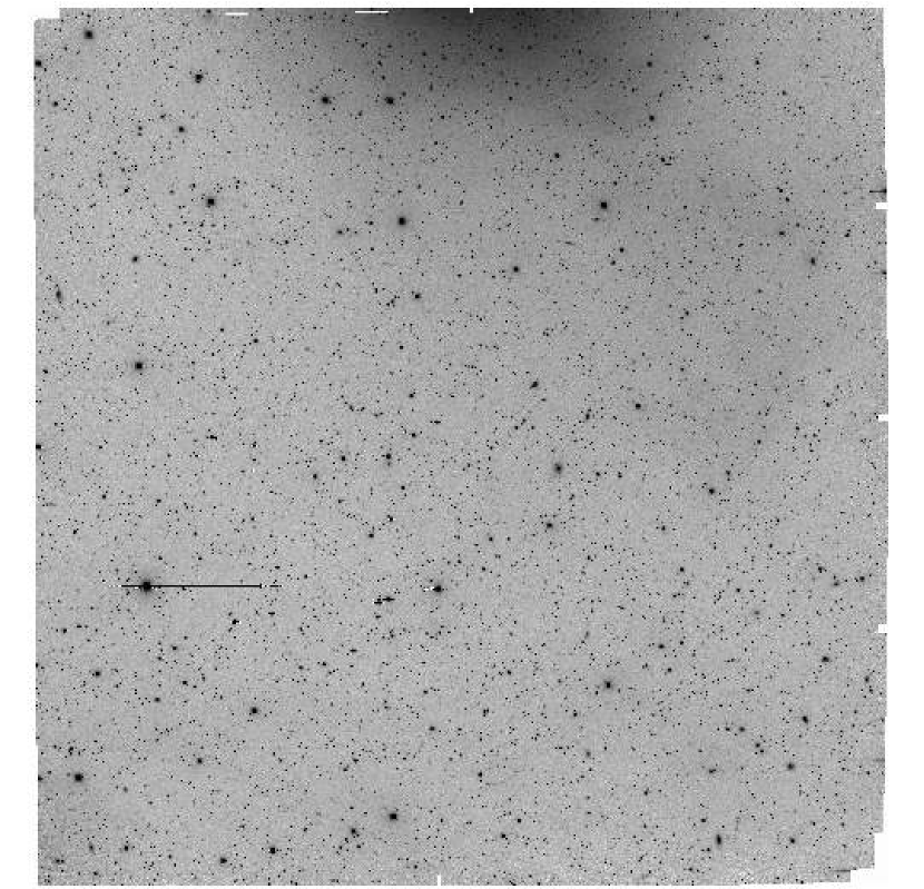
Figure 4.— V-band image of the S field.

3.2. Data Reduction

The CTIO Mosaic camera consists of eight $2048\times 4096$ CCDs arranged in a configuration that produces a $8196\times 8196$ pixel focal plane. We reduced the data using the IRAF tasks provided in the MSCRED package (Valdes 1998). These tools were specially designed for the reduction of mosaic CCD data. We applied standard techniques for CCD reduction, including overscan and bias subtraction, and flat-fielding. We took and used both dome, twilight, and night sky flats. We applied a sinc interpolation for astrometric regridding. The varying spatial scale in the field of view, where pixels farther from the image center subtend more sky, means that flat-fielding corrections overestimate the sensitivity of pixels at the field’s edge. The regridding process compensates for this effect and redistributes the flux properly.

Once images were regridded, we found it necessary to introduce another scaling correction. Due to either gain or linearity variations, the sky levels as traced across CCD boundaries were not continuous, having discontinuities of 0-3%. These were worst in the U and $B$ bands, especially for CCD 1 (the one in the lower left/southwestern corner). After determining that the bias levels could not have varied enough to cause these jumps, we decided to apply a scale factor correction to each CCD. While the presence of the galaxy makes it impossible to assume that the background is flat across the image, we can still assume that the background is continuous across the chip gaps. We made the assumption that CCD 2 is “truth” — this was the clear choice as most of our standard stars fell on CCD 2. While the halo (NE and S) fields required corrections in all filters, the CTR field only required corrections in the $U$ and $B$ band.

We independently checked the validity of these corrections by plotting the positions of stars in the various color-color diagrams, the “stellar locus”, for each chip assuming that the positon and tilt of the locus should not vary from chip to chip. Only with these corrections is the stellar locus seen to be identical in all chips. After implementing the CCD-dependent corrections, we median combined the dithered exposures for each field using 3-$\sigma$ rejection to create a final stacked image.

3.3. Photometric Solution

We observed sixteen standard stars each night from Landolt (1992) to perform the UBVRI photometric calibration. Observations in U and I for the NE and S field were taken under slightly non-photometric conditions on the first night, but these were subsequently calibrated on the second night. The photometric conditions were similar on nights 2 and 3, allowing us to apply the average photometric coefficients from both nights to all exposures. We assumed the mean UBVRI extinctions for CTIO with values 0.55, 0.25, 0.14, 0.10, and 0.08 magnitudes at the zenith, respectively.

One issue to be wary of when using mosaic cameras is the possibility that the different CCDs will have significantly different zeropoints and color terms. The best way to test this is to measure the same set of standard stars on each CCD. This is extremely time-consuming, and was not practical with the Mosaic’s 2.5 minute read-out. Instead, we used nine standards on CCD2 to determine the zeropoint in each band, and assumed the CCD2 color terms measured by the CTIO staff. The intra-CCD zeropoint offsets were determined using the method described in the previous section.

3.4. Object Detection and Photometry

We chose the widely used source detection program SExtractor (Bertin 1996) to create catalogs of objects in our three fields. SExtractor is well-designed for photometry of resolved objects on a variable background. This is the situation we face when we look for globular clusters superimposed on the smoothly variable galaxy light. We chose a mesh size (64 pixels or 16$\farcs$7) for the background estimation algorithm that was large enough to not affect the photometry of unsaturated objects, but small enough to follow the shell structure of NGC 5128 as well as subtract the wings of bright, saturated stars. The region in the central dust lane was too complex for reliable object detection and we ignored all objects detected there.

Photometry of all program field objects was done using a $3\arcsec$ diameter aperture. We corrected these measurements to $14\arcsec$ diameter apertures using the median growth curve of many bright, isolated stars. Aperture corrections were measure for each image so that seeing variations between images would not be an issue. We also examined the variation of the aperture correction as a function of spatial position in the image, and found that it was negligible for a $3\arcsec$ aperture. These corrections were typically on the order of 15%, or $-0.18$ mag. The $3\arcsec$ aperture was the best compromise between signal-to-noise, and the desire for the aperture correction to not vary significantly across the field-of-view. SExtractor detected objects on a summed $V+R$ image, and measured fluxes through the same apertures in all five bands.

Together in the three fields, we compiled a catalog of $56,674$ unique objects with good photometry—objects not corrupted by saturation, bleed trails, or edge effects—and $V<23$.

3.5. Comparison with Published Catalogs

While there have been many published photometric studies of this region, one of the most useful comparisons is with the VLT measurements of probable GCs in Rejkuba (2001). There are 78 objects for comparison in $U$ and $V$, 75 of which we detect (the remaining three were likely too faint). The $V$ photometry is well-behaved, as the errors are small for both studies. The median offsets between the Rejkuba and Mosaic photometry are small ($\sim 0.03$ mag), although the RMS scatter ($\sim 0.27$ mag) is higher than expected by about a factor of two. The $U$ is less consistent because our Mosaic observations do not go as deep as the VLT data. There is a $\sim 0.14$ mag offset between the two systems (our magnitudes are fainter), with $\sim 0.3$ mag RMS scatter. If significant, this difference could be a result of slightly different calibrations or aperture corrections. Globular clusters at the distance of NGC 5128 may also be slightly extended in appearance. Because our aperture corrections are derived from stellar profiles, we may underestimate the total flux of the more extended GCs by as much as $\sim 0.1$ mag, although a more typical value would be $\sim 0.06$ mag. However, this effect is much smaller on GC colors since the seeing did not vary much across most of our observations. Because the science goals of this study focused mostly on the relative colors of the GCs, we chose to defer a more precise treatment of GC light profiles to a later study.

Table 2Observing Runs: Spectroscopy

Target(s)	Instrument	FOV	Fibers	Grating	Res	Date
		(′)			(Å)
PN/GC	AAO/2dF	120	400	1200B	2.2	2001 Jan 20
PN/GC	CTIO/Hydra	40	130	KPGL3	4.9	2001 Feb 18–20
PN/GC	AAO/2dF	120	400	1200V	2.2	2002 Apr 4–6, 9–10

Comparisons with the UBVR photoelectric photometry of Zickgraf et al. (1990) show that our photometry is consistent with their published values. We also checked against the list of confirmed GCs in HGHH92 and other previous work. This sample is considerably brighter than that of Rejkuba (2001) and we detect all known GCs that are in our field of view.

4. Building a Catalog of Globular Clusters

4.1. A Spectroscopic Survey

Determining which of our detected objects are actually GCs in NGC 5128 is a non-trivial task. While the total number of GCs in NGC 5128 is estimated to be 1200–1900 (G.Harris et al. 1984), there are 17,407 unique objects in our catalog that fall in the magnitude range that corresponds to the bright half of the globular cluster luminosity function (GCLF) $14.0<V<20.5$. Our faint end cut off for spectroscopy is approximately the magnitude of the GCLF peak, yet we estimate that only 3–$6\%$ of objects in this magnitude range are GCs. With such a high level of contamination from foreground stars (background galaxies are not so important at these relatively bright magnitudes), it is difficult to know which objects are really GCs.

Some of the more extended GCs will be resolved in our ground-based imaging (at the distance of NGC 5128, $1\arcsec\approx 17~{}$pc); W.Harris et al. (2002) used HST imaging to determine that GCs in NGC 5128 have characteristic half-light radii of $0\farcs 3-1\farcs 0$. While size and morphology can be used as leverage in selecting high-probability GCs, radial velocities are the best way to distinguish between GCs and foreground stars. The systemic velocity of NGC 5128 is 541 km s^-1 (Hui et al. 1995), which means that most GCs will have radial velocities larger than those of Galactic stars. The central stellar velocity dispersion of NGC 5128 is $\sim 140$ km s^-1 (Wilkinson et al. 1986). Assuming that the GC system has a gaussian line-of-sight velocity distribution with a similar dispersion, introducing a velocity cutoff at $v_{r}>250$ km s^-1 excludes only the lowest $1.9\%$ of the GC velocity distribution. The PN radial velocity distribution is consistent with this, as only eight of 780 PNe in NGC 5128 ($1.0\%$) have $v_{r}<250$ (Peng, Ford, & Freeman 2004). Even at this velocity cutoff, however, there is a chance that a few high-velocity Galactic halo stars will contaminate our sample. The sun’s direction of motion in the disk is generally away from NGC 5128, so the velocity conversion from the the Galactic standard of rest to the heliocentric frame is substantially positive ($+161$ km s^-1). Even so, only a small fraction of the Galactic halo star distribution presents any possible contamination.

Prior to this work, there were only 77 GCs with published velocities. These were from a series of papers (VHH81, HHH86, HGHH92), the latter of which included 32 velocities from the sample of Sharples (1988). A number of papers (MAGJM96, HCH99, Rejkuba 2001, W.Harris et al. 2002) subsequently published lists of probable GC candidates in small fields based on imaging data alone. However, it is important to obtain velocities to be more certain of the nature of these objects. Modern fiber spectrographs on southern telescopes, such as the 2-degree Field spectrograph (2dF) on the 3.9-meter Anglo-Australian Telescope, and the Hydra spectrograph on the CTIO Blanco 4-meter telescope, are well-suited to a radial velocity survey in the halo of NGC 5128.

4.2. Observations

We confirmed GCs and refined our target selection over the course of three spectroscopic observing runs. Our first and third runs were with 2dF. The first was in January 2001 during dark time, and the third was in April 2002 in gray time. The eponymous two degree diameter field of view of 2dF is filled with 400 fibers. Our second observing run was with the CTIO-Hydra spectrograph. Hydra is similar to 2dF, except that it has a smaller field of view ($40\arcmin$ diameter) and $\sim 130$ fibers. These observing runs are listed in Table 2. In all of these runs, PNe were also targeted. In addition to our primary aim of discovering new GCs, we tried to confirm the nature of published high-probability GCs — the brighter candidates from MAGJM96, HCH99, and Rejkuba (2001). We also observed many of the HGHH92 GCs for consistency, and in some cases to get more accurate velocities.

These data were reduced using standard packages and techniques for fiber spectroscopy. Details of the reduction are given in a companion paper on the planetary nebula system of NGC 5128 (Peng, Ford, & Freeman 2004). Unlike for PNe, we do not gain in S/N by going to higher dispersion. For 2dF observations with the 1200V grating ($2.2$ Å per resolution element), we subsequently smoothed our GC spectrum by a three pixel boxcar. The resulting resolution was comparable to our setup with Hydra and did not noticeably compromise our velocity accuracy. Sky-subtraction, which is not essential for PNe, was performed on the GC spectra.

Also unlike in the case of PNe, we performed radial velocity measurements on GCs using the Fourier cross-correlation method implemented in the fxcor task of the IRAF radial velocity package. During our CTIO-Hydra run, we observed the radial velocity standard HR 5196, which has a published velocity of $-39.598$ km s^-1 (Skuljan, Hearnshaw, & Cottrell 2000), but stars are not always optimal templates for cross-correlating with globular clusters. We used HR 5196 to check the velocity of a high S/N Keck spectrum of an M31 GC, and we subsequently used this GC as our velocity template.

4.3. Target Selection: Morphology

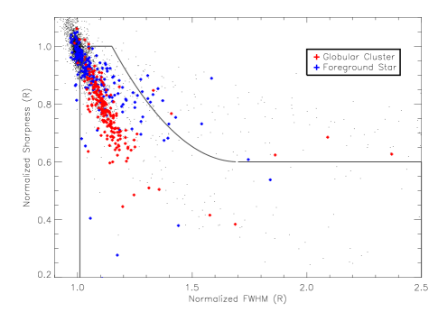
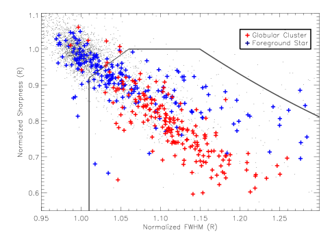
Figure 5.— GC selection using normalized sharpness and FWHM. Sharpness is the ratio of peak flux to total flux. Both quantities have been normalized to local values. The black line outlines our rather generous selection boundary. Objects become more extended as they move to the lower right. (a) The top panel shows all candidates for the CTR field as well as confirmed GCs and stars. (b) The bottom panel shows a zoom in of the upper left region.

Even with the 400 fibers on 2dF and the 130 fibers on Hydra, we cannot take a spectrum of every object in the expected magnitude range. Thus, it is important that we develop an efficient algorithm to select likely GCs. We developed our target selection algorithm using structural parameters and colors. With the best seeing in each field being nearly $1\arcsec$, it is possible to resolve some of the more extended GCs in our imaging. We use two structural parameters, sharpness and full-width at half maximum (FWHM), in conjunction with ellipticity to identify round, extended objects in our catalog. We define sharpness to be the ratio of flux in the brightest pixel to the “total” flux — that measured within the SExtractor automatic Kron aperture. This is essentially a difference of aperture magnitudes that measures the concentration of the object. This approach benefits from a nicely oversampled PSF (5 pixels per FWHM). Because the point spread function varies across the field-of-view, we normalized both sharpness and FWHM to the local value. Thus, objects that are extended have normalized sharpnesses less than unity, and normalized FWHMs greater than unity.

Figure 5 shows plots of normalized sharpness versus normalized FWHM for the CTR field. The bottom plot is a zoomed-in version of the top. The black dots are objects in the CTR field with $V<20.5$ and $U<23$. Most of the objects cluster around (1,1), as we would expect for a sample dominated by stars. However, there is a fan of points toward lower sharpness and higher FWHM. Overplotted in red are all spectroscopically confirmed GCs, and in blue are all spectroscopically confirmed foreground stars. This is not the training set we had to work with initially, but we plot the end-product catalog for the purpose of demonstration. It is also important to remember that when we first decided on our cuts, we based our selection on the 63 HGHH92 GCs and some of the brighter high-probability GCs from Rejkuba (2001). We did not have a sample of confirmed foreground stars until after our first spectroscopic run. Results from each observing run were used to improve the selection for subsequent runs.

Table 3Spectroscopic Follow-up of GC candidates

		Total	Newly Confirmed GCs					Known GCs
Facility	Dates	Targets	Mos	HHH	R01	MAGJM	HCH	HGHH
AAO/2dF	2001 Jan 20	120	2	0	0	0	0	28
CTIO/Hydra	2001 Feb 18–20	254	88	2	28	4	6	7
AAO/2dF	2002 Apr 4–6, 9–10	59	19	0	0	0	0	8

The GCs are clearly in a locus offset from the stars. This morphological selection bias has been built into the sample—most known GCs in earlier work and our study were selected at least in part because of their spatial extent—yet it shows that at least some GCs can be separated from stars given the seeing in our images. Not all stars are concentrated at (1,1), as there is a tail of stars to higher FWHM. These stars, however, are typically sharper for their FWHM than are the GCs. Upon visual inspection, we found that the locus of sharp but extended points primarily consist of unresolved blends. One disadvantage of using SExtractor is that with only one iteration of object detection and no PSF subtraction, it cannot detect faint stars that are very close to brighter ones. The bottom plot illustrates more clearly how the loci of stars and GCs separate in sharpness at larger FWHM.

The lines in Figure 5 denote the area within which we accepted an object as a GC candidate for our second and third spectroscopic runs (there was no sharpness/FWHM cut for the initial run). First, we exclude most of the stellar locus. The top line that asymptotes to a normalized sharpness of 0.6 excludes the most egregious blends from being targeted (although it may also exclude star-GC blends). While the GCs actually form a fairly tight sequence in this plot, we chose to be conservative and allow more stars into the selection area to increase our completeness. The last morphological cut was a relatively loose one that rejected all objects with ellipticities greater than 0.4. Almost all GCs have ellipticities less than 0.1, so this cut simply rejected obvious background galaxies, and also served to eliminate partially resolved pairs of objects.

4.4. Target Selection: Optical Colors

In addition to selecting on size and shape, we instituted color cuts to increase our efficiency. Globular clusters are old, single-age stellar populations that have optical flux predominantly produced by stars from the main sequence turnoff to the red giant branch. The integrated colors of these stellar populations are produced by combinations of stars with types F through K (and maybe also A-type giants for GCs with blue horizontal branches). The result is that the spectral energy distribution of a GC is broader than that for any individual star. Hence, with a long enough wavelength baseline and sufficiently accurate photometry, we should be able to distinguish GCs from stars using colors alone.

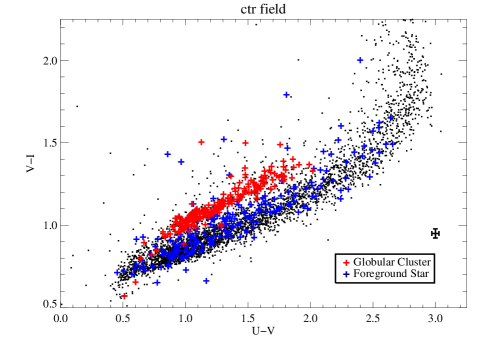
Figure 6.— Color separation for GCs and stars in $UVI$ Black dots are objects in our CTR field with $14<V<20.5$. The error bars are representative for bright object photometry. Globular clusters are offset from the stellar locus in the way one would expect if they had a composite stellar population. Discrepant GCs with ($V$–$I$)$\sim 1.5$ have large photometric errors.

Figure 6 shows a ($U$–$V$)–($V$–$I$) color-color diagram—the combination of colors that offers the widest wavelength baseline for our data. The black dots are objects in our CTR field with $14<V<20.5$. The dense concentration of points outline the $UVI$ stellar locus. As in Figure 5, all confirmed stars and GCs are overplotted as blue and red plus symbols, respectively. Although the division is not perfect, there is a clear separation between GCs and stars in $UVI$ color space—at a given $U$–$V$, GCs are redder in $V$–$I$. $U$-band photometry, though expensive, is valuable for the separation of GCs from stars.

4.5. Spectroscopic Yields

The results of these three spectroscopic runs are summarized in Table 3. The total numbers of clusters listed will be larger than the numbers in the final catalog because some were observed in multiple runs. We took slightly different targeting strategies in each run. For the first 2dF observations, GC candidates were piggybacked onto observations of PNe. PNe had the highest priority while GC candidates were used to fill empty fibers in the uncrowded halo regions. Most of these candidates were in the NE field, and we used only broad color cuts, no morphology cuts, and a magnitude limit of $V<20$. This selection produced very few new GCs (only a 2% yield), because the color cut included a large portion of the stellar locus, and the candidates were restricted being the NE halo field where the density of GCs is low. Our three night Hydra run also combined PNe and GCs, although GCs received the higher priority. This time, we implemented a cut on normalized sharpness and FWHM, combined with a weak cut on color. Our third observing run was another where we targeted both PNe and GCs. For this fiber configuration, we implemented a combined $UVI$ and morphology cut, and also extended the magnitude ranges to $V<20.5$. The yield of new GCs was $\sim 40$% for both of these runs, showing that careful selection criteria can increase efficiency by an order of magnitude. The results of our observing program are shown in the selection diagrams of Figures 5 and 6.

5. Galaxy Background Subtraction

For the purposes of measuring line indices (and to a lesser extent, radial velocities), it is important to determine the fraction of light that went through the fiber that is from the targeted globular cluster. The nature of fiber spectra is such that background subtraction is not local. Typically, thirty or more sky fibers are placed at positions free of objects, and their spectra are combined to create a master sky spectrum. This spectrum is then scaled to each individual object spectrum, either using sky lines or measured throughput differences, and then subtracted. This approach works well (to within 1–2%) when the background is relatively constant. However, in the case of our observations around NGC 5128, the background in regions near the galaxy center is a spatially varying combination of the sky and the unresolved galaxy light. This is not a problem for slit spectra where the local background is determined for each object individually in spatially adjacent regions. This does become a problem for fiber spectra where no single composite sky spectrum is representative for the entire field of view. Since sky fibers are given lower priority and are often placed away from the galaxy center (where there is less crowding from program objects), sky fibers typically contain little galaxy light. Thus, the spectra of faint, centrally located GCs may have a significant contribution from the field light of the galaxy. For line index measurements in particular, it is important that these GCs have the galaxy contribution removed from their spectra.

With the GC fiber spectra alone, this would be a difficult problem. The many different aspects of our data set, however, permitted us to develop a workable solution. First, when creating the composite sky spectrum, we used only those sky spectra that showed no visible contribution from the galaxy so that it was pure sky. This was not a problem as, again, most sky fibers were placed well away from the bright parts of the galaxy. After sky subtraction, the reduced program spectra are some combination of cluster and galaxy. Using our imaging in the $B$ and $V$ bands, we measured the fraction of light down each fiber (2″ diameter) that should belong to the galaxy. The distribution of this galaxy fraction for the Hydra-observed GCs is shown in Figure 7. It is reassuring that most of the GCs have only a low level of galaxy contamination (median of 11%), and almost all have contamination lower than 50%.

Figure 7.— Fraction of galaxy light down each fiber for GC spectra (Hydra sample). Using $B$ and $V$ images, we calculated the fraction of light that went down each 2″ diameter fiber that originated from the galaxy’s unresolved stellar light. Most spectra are relatively free of galaxy contamination.

In order to subtract the galaxy’s contribution to each spectrum, we created a template galaxy spectrum. By summing the sky fibers that have visible galaxy signal even when the master sky spectrum has been subtracted—those targeting “sky” regions toward the center of the galaxy—we obtained a high S/N galaxy composite. By scaling this composite to the galaxy fraction computed with the imaging data, we are able to remove the underlying galaxy contribution.

The last variable is the velocity and velocity dispersion of the galaxy at the location of each fiber. Because the rotation in the mean velocity field can cause the galaxy spectrum to shift by $\pm 1.5$Å, it is important that the scaled spectrum be redshifted to the proper velocity before subtracting it. For this, we use the mean velocity of the planetary nebulae (PNe) at each fiber location (Peng, Ford, & Freeman 2004). Because PNe trace the kinematics of the old stellar population, and the field should be smoothly varying, this is a valid method of estimating the local mean velocity field. The velocity dispersion can be assumed to be constant for these purposes.

After redshifting and scaling the composite galaxy spectrum for each GC, we removed the bulk of the galaxy’s signature in each spectrum. While this technique removes zeroth order contributions from the galaxy, it can introduce small errors. If the seeing is different during the spectroscopic observing run than during the imaging, then the computed galaxy fraction will be slightly off. For example, if the seeing for the imaging was $1\farcs 2$ but the seeing for spectroscopy was $1\farcs 5$, then a GC with a calculated galaxy contamination of 11% will instead have a true contamination of 13% due to more of the GC light being outside the fiber aperture. Also, since the composite galaxy spectrum is a mixture of light from different regions in the galaxy, it does not take into account spatial variations in metallicity and age that may cause the background to vary. However, without a spectroscopic measurement of the local background, by either using slits or chopping to local sky, this is probably the best background subtraction we can achieve. Figure 8 shows an example of this subtraction in the $V=18.0$ cluster, pff_gc-068, a case where the galaxy fraction is fairly high ($\sim 0.3$). In addition, the galaxy fraction distribution (Figure 7) shows that few GCs are like the example in Figure 8 and so this procedure is important for only a subset of GCs.

Figure 8.— An example of galaxy subtraction. This star cluster’s spectrum has a high contamination from galaxy light. The original spectrum is shown in black (top) with the scaled and redshifted galaxy spectrum in red (bottom), and the final subtracted spectrum in blue (middle). Notice how the galaxy template is broader and slighted shifted from the cluster spectrum.

Over half of our spectroscopic sample with Mosaic photometry (136 GCs) was observed with CTIO/Hydra. This is the only observing run for which we obtained high signal-to-noise spectra of the galaxy and Lick/IDS standard stars. These spectra also had the largest wavelength coverage (3800-5500Å). Therefore, we only performed galaxy subtraction and line index measurements on the CTIO/Hydra sample. All Hydra spectra had their radial velocities re-measured after galaxy subtraction, but the changes were minimal — a few km s^-1 at most.

6. Catalog

6.1. The Globular Cluster Catalog

The final globular cluster catalog contains 215 unique globular clusters in NGC 5128 from various sources. Of these, 138 are newly confirmed GCs that have no velocities in the published literature. In each of our spectroscopic runs, we re-observed objects from previous runs to provide a consistent velocity zeropoint. We also re-observed GCs with published velocities (HGHH92) for comparison. These repeat observations are important for creating a consistent velocity catalog, and for quantifying our velocity errors. We present these data in Table 4.

Table 4GC Velocity Offsets and Errors from Repeat Observations

Velocity Source	Offset	RMS	No. Overlap	$<V>$
	(km s-1)	(km s-1)
Hydra 2001	0	0	N/A	N/A
2dF 2001	$2\pm 15$	48	10	19.1
2dF 2002	$-14\pm 10$	65	22	19.4
HGHH92	$-26\pm 24$	85	12	18.6
HGHH92	$-26\pm 14$	73	28	18.7

We chose to compare all velocities to the Hydra observations, the only observing run for which we obtained a radial velocity standard. The offsets between Hydra and the two 2dF runs are negligible, and consistent with zero. The offset between our data and the published velocities in HGHH92 is approximately $-26$ km s^-1. While the dispersion for these HGHH92 GCs is considerably higher, the offset is marginally significant. The dispersions for the repeat velocity data vary from 48–85 km s^-1. This can be explained by the data quality of the different repeat samples. The mean $V$-magnitude of the twelve overlap objects between the Hydra and 2001 2dF runs is 0.6 mag brighter than the mean $V$-magnitude of the overlap objects between Hydra and the 2002 2dF run. Many of the 2002 2dF observations were also taken during fairly bright moon. Assuming that the Hydra and 2dF observations have similar errors that add in quadrature, we derive a velocity error of 34 km s^-1 for objects with $V<19$. This is consistent with the median velocity error of our sample as derived from the Fourier cross correlation technique. For fainter GCs, however, the velocity error can be as large as 70 km s^-1.

The large velocity dispersion between our data and the HGHH92 published velocities are not likely due to low S/N. The mean magnitudes of these overlap GCs are well in the high S/N regime. Given the accuracy of our other repeat measurements, it is likely that the intrinsic errors of the HGHH92 velocities are $\sim 65$ km s^-1. Therefore, when incorporating the HGHH92 GCs into our final catalog, we always replace the published velocity with our own measurement if it exists. If we did not observe a given HGHH92 GC, then we use the published velocity with an offset of $-26$ km s^-1, as shown in Table 4.

We visually evaluated the quality of each spectrum and radial velocity. For objects with multiple observations, we retained the velocity derived from the highest S/N spectrum. In cases where the S/N was comparable for all observations, we used the weighted mean of the observed values.

In Table 5, we present the final GC velocity catalog. For each object, we list its coordinates, UBVRI photometry (if it exists) and its final heliocentric radial velocity. Column 1 is the name of the object; Columns 2 and 3 are the RA and Dec coordinates in J2000.0 on the USNO-A2.0 astrometric reference frame; Column 4 is $R_{p}$, the projected radius in arc minutes; Columns 5 and 6 are $X$ and $Y$, NGC 5128-centric coordinates that are arc minutes along the photometric major and minor axes, respectively, where the major axis is taken to have a position angle of 35°; Column 7 is the $V$ magnitude; Columns 8–11 are the U B, B V, V R, and $V$–$I$ colors; Columns 12–16 are the associated photometric errors; Column 17 is . $V_{h}$, the heliocentric velocity; Column 18 is $V_{h,err}$, the error in the measured velocity, or if the velocity is from the literature, then we assume an error of 65 km s^-1; Column 19 is $E_{B-V}$, the reddening for each GC as derived from the maps of Schlegel, Finkbeiner, & Davis (1998). Column 20 is the “Run”, which designates during which observing run(s), if any, the object was observed, where the runs are numbered such that “1” is the 2dF 2001 run, “2” is the Hydra 2001 run, and “3” is the 2dF 2002 run.

We always give GCs the primary designation from the earliest publication in which it appears (except for GP80-1), and we have done our best to match duplicates. Rejkuba (2001) GCs are labeled by and “R”, then by a 1 or 2 depending on whether they were in her fields 1 or 2, then by the two digit number that she gave them. All GCs that have a VHH81 or HGHH designation had previously published velocities. All GCs with an HHH86 designation, except for HHH86-13 and HHH86-15, also had published velocities. The remaining GCs are newly confirmed. A few GCs have multiple names in the published literature. This is true for a few Rejkuba (2001) GC candidates, where R226 is HHH86-15, R123 is HHH86-38, R281 is HGHH-12. The GC from Graham & Phillips (1980) is also HGHH-07.

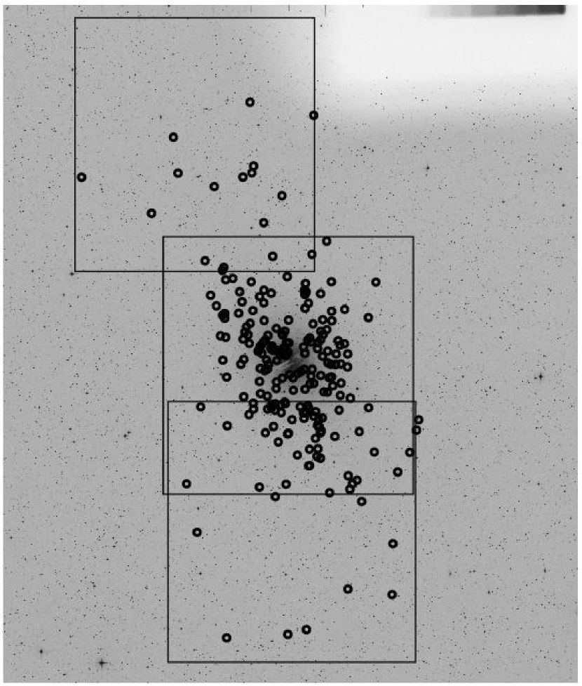
Figure 9.— GC positions and Mosaic fields overplotted on a DSS image of NGC 5128.

Figure 9 shows the locations of all confirmed GCs with respect to the galaxy and the three Mosaic fields. While the farthest GCs are at projected radii greater than 40 kpc, slightly over half are contained within $2r_{e}$, where $r_{e}=5.2$ kpc. The median projected radius of the GCs in our sample is $\sim 9$ kpc.

6.2. Foreground and Background Objects

Table 6 lists all confirmed foreground stars in the halo of NGC 5128. This table is included so that future astronomers looking for GCs in NGC 5128 need not experience the disappointment of re-observing them. Note that while almost all observed Rejkuba (2001) candidates are true GCs, f1.gc-19 (R119) is actually a star. The column labels are the same as for Table 5, except that the columns containing $R_{p}$, $X$, and $Y$ are not included. The combined velocity distributions of these two samples is shown in Figure 10.

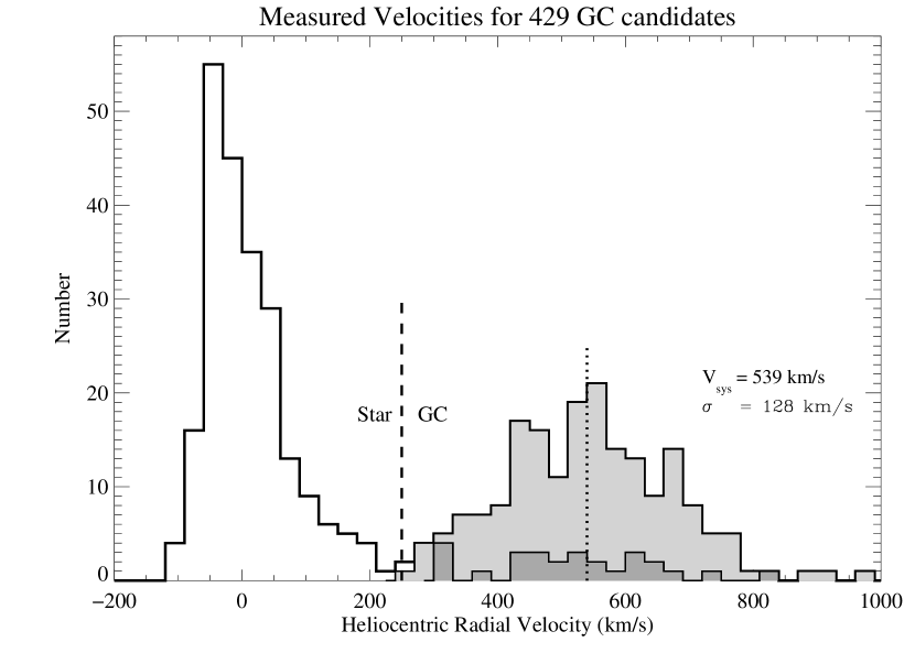
Figure 10.— Velocity Distribution of Cluster Candidates. A histogram of velocities for all objects targeted as globular cluster candidates. The foreground star contamination is apparent, as is the population of true Cen A globular clusters. While there may be a few misclassified objects, the two populations are well-separated in velocity. Objects at radial velocities between 250 and 1000 km/s are classified as clusters. The black line is the histogram for objects observed in our program, with the light gray shading representing the GCs. The underlying dark gray histogram is the fraction of our observed sample that was previously confirmed (from VHH81, HHH86, and HGHH92). This does not represent the full sample because we did not reobserve all known GCs. The mean systemic velocity of the GC system is 539 km s^-1, which is observationally indistinguishable from the systemic velocity derived from the PNe.

We also list GC candidates that were neither GCs nor stars. This was the case for very few objects, but in some cases, candidates turned out to be background galaxies. These are listed in Table 7. Redshifts were determined from one or more spectral features such as [O II], [O III], or Ca H and K, and are good to within 0.01. Column labels are the same as for Table 6.

6.3. Matches with X-Ray Point Sources

Using Chandra data, Kraft et al. (2001) produced a list of 246 X-ray point sources within a couple effective radii in NGC 5128. Many X-ray point sources in old stellar populations have optical matches that are globular clusters (Kundu, Maccarone, & Zepf 2002), and it is believed that GCs may be the dominant sites for the formation of low-mass X-ray binaries. We present 52 optical matches to the Kraft et al.  catalog from our photometry. We matched objects within a $3\arcsec$ radius, that had $17<V<21.5$ and were not in the dust lane. Thirteen of these are known GCs, and the others are likely to also be GCs. The full list is presented in Table 8. Column labels are the same as for Table 6 except that Column 1 contains the ID from Kraft et al. (2003), Column 2 is the ID given from any previous GC survey, and we do not include columns for $R_{p}$, $X$, $Y$, $V_{h}$, or Run. Like others, we find that the optical counterparts to X-ray point sources are more likely to have colors consistent with metal-rich GCs than metal-poor GCs. A thorough analysis of the nature of the optical-X-ray sources in NGC 5128 is presented with complementary data by Minniti et al. (2003).

6.4. Serendipity: White Dwarfs and QSOs

In addition to looking for old GCs, we used some fibers to specifically target blue objects in the NGC 5128 field in the hopes of finding young clusters in the halo, like the one in the young tidal stream described in Peng, Ford, & Freeman (2002). We implemented a simple magnitude cut $V<20.0$, and color cut $(B-V)_{0}<0.285$, assuming a foreground reddening $E(B-V)=0.115$ mag (Schlegel et al. 1998). While we did not find any unambiguous young clusters in the halo, we did discover low-redshift emission-line galaxies, metal-poor dwarf stars, white dwarfs and QSOs. Three white dwarfs and seven QSOs are listed in Table 9. Columns are similar to Tables 5–8, except the redshift of QSOs is listed in Column 9. The white dwarfs were identified by their broad H$\beta$ absorption, and the QSOs by their Mg II emission. Occasionally, intervening Mg II absorbers were visible blueward of the Mg II emission. None of these lines are likely to be Lyman-$\alpha$, because in all cases, there is detectable continuum blueward of the emission line. Redshifts were determined using the Mg II emission line, and are good to 0.05. Our relatively narrow wavelength range restricted us to identifying QSOs with redshifts around $z\sim 0.7$. Although these QSOs are not especially bright ($V>19$), they seem to have smooth continua and may eventually be useful for probing the interstellar medium in the halo of NGC 5128.

7. The Reported Planetary Nebula in HGHH-G169

Figure 11.— A 2dF spectrum of HGHH-G169. We zoom on the [OIII]$\lambda\lambda 4959,5007$ lines to show that they are split by roughly 5Å (300 km s^-1).

In the course of obtaining spectroscopy for GCs in NGC 5128, Minniti & Rejkuba (2002, MR02) found that the GC HGHH-G169 had strong [O III] emission in its spectrum. They concluded that it was a planetary nebula within the GC—the first of its kind in an elliptical. PNe are extremely rare in Galactic globular clusters, and it would be exciting if more GC-associated PNe could be located in other galaxies.

During the course of our survey, we also observed HGHH-G169. Like MR02, we targeted it (in our 2001 2dF run) because it is listed in HGHH92. We also noticed strong [O III] emission in the GC spectrum, and thought it might be a PN. However, we were somewhat puzzled because both [O III] lines ($\lambda\lambda 4959,5007$) are double-peaked, with the separation between the peaks being about 5Å (300 km s^-1). The [O III] region of the spectrum is shown in Figure 11.

We carefully checked the raw data to test the validity of this split. The split lines are seen in all five of the pre-combined frames, and the arc calibrations show only single peaks. Hence, we are convinced that this split is real. Moreover, it is unlikely that MR02 would have been able to resolve these lines. With the Boller and Chivens spectrograph on the Magellan Baade telescope, they likely had 6Å instrumental resolution. Our 2dF resolution was 2.2Å.

If we assume that the line splitting is due to seeing the front and back sides of an expanding shell (with an expansion velocity of  150 km/s), then it is unlikely that this object is a PNe. Planetary nebulae normally have expansion velocities of only a few tens of km s^-1. In addition, the spectrum displayed in MR02’s Figure 2 (top) shows hints of He I$\lambda 5876$ and [O I]$\lambda 6300$ emission. If these low-excitation lines are confirmed, then this object is unlikely to be a PN. We think that the different ionization states and the fast expansion velocity makes it possible that this is a supernova remnant, which would also be very interesting.

We also have ground-based [O III] narrow-band and continuum images of this region from the survey of H93. Despite its strong [O III] flux, this object would not have met H93’s or our selection criteria because we require that there be no detection in the continuum image; in this case, there is a bright GC visible in the off-band at that position. Upon close inspection, the source of the [O III] emission is offset by $\sim 1\farcs 4$ northeast of the center of HGHH-G169, which translates to a physical distance of 24 pc. While this is still close enough to be associated with HGHH-G169, the object would need to be toward the outskirts of the cluster.

Whether or not this object is a PN, it is still interesting and highlights the need to inspect GC spectra for other features. While some of the GCs near the dust lane have spectra that contain low excitation emission lines, this is likely to be due to the star formation that is ongoing in the region rather than from emission within the GC. None of our other spectra showed signs of having a planetary nebula. As MR02 discuss, these numbers are starting to place some statistically interesting constraints on the formation of PNe in globular clusters.

8. Summary

We conducted an optical imaging and spectroscopic survey for globular clusters across $\sim 1\arcdeg$ of sky around NGC 5128. Using UBVRI photometry, size, and morphological information, we developed an efficient algorithm for selecting likely GCs candidates for spectroscopic follow-up—a necessity given the large number of foreground stars. We obtained radial velocities for over 400 objects. Of these, we identified 102 previously unknown GCs, confirmed the nature of 24 GCs from Rejkuba (2001), 6 GCs from HCH99, 4 GCs from MAGJM96, and 2 from HHH86, providing 138 new GC velocities. We also obtained new velocities for 25 previously confirmed GCs from HGHH92 and HHH86. The total number of confirmed GCs in NGC 5128 is now 215.

We present a spectrum of HGHH-G169, which shows an interesting split emission line feature. It is unlikely to be a planetary nebula, as MR02 suggest, but it could be a supernova remnant, and certainly merits a deeper spectrum.

Table 5Catalog of NGC 5128 GCs with Radial Velocities.

Name	RA	Dec	$R_{p}$	$X$	$Y$	$V$	$U$-$B$	$B$-$V$	$V$-$R$	$V$-$I$	$\sigma_{U}$	$\sigma_{B}$	$\sigma_{V}$	$\sigma_{R}$	$\sigma_{I}$	$V_{h}$	$V_{h,err}$	$E_{B-V}$	Run
	(J2000)	(J2000)	(′)	(′)	(′)	mag	mag	mag	mag	mag	mag	mag	mag	mag	mag	km/s	km/s	$E_{B-V}$
pff_gc-001	13:23:49.62	$-$43:14:32.0	22.38	$-21.290$	$6.903$	18.91	0.47	1.01	0.55	1.31	0.09	0.02	0.01	0.01	0.03	722	52	0.14	2
pff_gc-002	13:23:59.51	$-$43:17:29.1	22.96	$-22.660$	$3.728$	19.55	0.27	0.88	0.53	1.11	0.07	0.02	0.01	0.01	0.03	623	52	0.14	2
pff_gc-003	13:24:03.23	$-$43:28:13.9	31.19	$-31.047$	$-3.025$	19.31	0.21	0.87	0.51	1.09	0.15	0.02	0.01	0.01	0.03	697	23	0.13	3
pff_gc-004	13:24:03.74	$-$43:35:53.4	38.00	$-37.248$	$-7.519$	20.01	0.28	0.83	0.52	1.09	0.28	0.03	0.01	0.01	0.03	546	45	0.13	3
pff_gc-005	13:24:18.92	$-$43:14:30.1	18.36	$-18.185$	$2.563$	20.29	0.58	1.02	0.58	1.22	0.18	0.04	0.01	0.01	0.03	756	34	0.14	3
pff_gc-006	13:24:23.72	$-$43:07:52.1	13.51	$-12.260$	$5.671$	19.22	0.21	0.78	0.52	1.02	0.05	0.02	0.01	0.01	0.03	641	41	0.13	2
pff_gc-007	13:24:24.15	$-$42:54:20.6	13.45	$-1.160$	$13.399$	20.12	0.69	1.04	0.59	1.30	0.17	0.03	0.01	0.01	0.03	612	28	0.13	3
pff_gc-008	13:24:29.20	$-$43:21:56.5	23.42	$-23.188$	$-3.252$	19.94	0.47	0.99	0.54	1.19	0.35	0.03	0.01	0.01	0.03	451	43	0.14	3
pff_gc-009	13:24:31.35	$-$43:11:26.7	14.59	$-14.382$	$2.473$	19.77	0.23	0.81	0.52	1.07	0.07	0.02	0.01	0.01	0.03	657	46	0.13	2
pff_gc-010	13:24:33.09	$-$43:18:44.8	20.27	$-20.169$	$-1.991$	19.68	0.09	0.68	0.42	0.85	0.06	0.02	0.01	0.01	0.03	344	58	0.13	2

Note. — There are 215 confirmed GCs, of which the first ten are listed here. The complete version of this table is in the electronic edition of the Journal. The printed edition contains only a sample.

Table 6Catalog of Confirmed Foreground Stars in Vicinity of NGC 5128

name	RA	Dec	$V$	$U$-$B$	$B$-$V$	$V$-$R$	$V$-$I$	$\sigma_{U}$	$\sigma_{B}$	$\sigma_{V}$	$\sigma_{R}$	$\sigma_{I}$	$V_{h}$	$V_{h,err}$	Run
	(J2000)	(J2000)	mag	mag	mag	mag	mag	mag	mag	mag	mag	mag	km/s	km/s
pff_fs-001	13:23:50.43	$-$43:27:28.3	18.05	0.17	0.70	0.41	0.83	0.06	0.01	0.01	0.01	0.03	$-93$	$18$	2
pff_fs-002	13:23:50.74	$-$43:35:02.6	19.28	0.71	1.10	0.65	1.47	0.32	0.02	0.01	0.01	0.03	$-51$	$31$	23
pff_fs-003	13:23:51.83	$-$43:37:00.1	19.01	0.17	0.71	0.42	0.91	0.12	0.02	0.01	0.01	0.03	$-44$	$31$	3
pff_fs-004	13:23:52.56	$-$42:42:33.5	19.72	0.19	0.67	0.68	1.43	0.10	0.03	0.01	0.01	0.03	$71$	$28$	3
pff_fs-005	13:23:54.36	$-$42:48:17.7	19.42	$-$0.09	0.70	0.34	0.92	0.05	0.02	0.01	0.01	0.03	$200$	$48$	3
pff_fs-006	13:23:55.77	$-$43:13:15.2	20.15	0.99	1.23	0.76	1.52	0.24	0.04	0.01	0.01	0.03	$-59$	$26$	3
pff_fs-007	13:24:02.70	$-$42:49:54.3	20.04	0.35	0.83	0.49	1.05	0.10	0.03	0.01	0.01	0.03	$-84$	$24$	3
pff_fs-008	13:24:02.76	$-$43:30:15.5	18.18	0.24	0.83	0.53	1.13	0.07	0.01	0.01	0.01	0.03	$-66$	$18$	2
pff_fs-009	13:24:03.70	$-$43:12:13.6	20.32	1.33	1.27	0.69	1.49	0.39	0.05	0.01	0.01	0.03	$-45$	$23$	3
pff_fs-010	13:24:03.81	$-$43:28:05.9	19.40	1.19	1.23	0.72	1.42	0.52	0.02	0.01	0.01	0.03	$-3$	$24$	2

Note. — There are 222 confirmed foreground stars, of which the first ten are listed here. The complete version of this table is in the electronic edition of the Journal. The printed edition contains only a sample.

Table 7Catalog of Confirmed Background Galaxies in Vicinity of NGC 5128

name	RA	Dec	$V$	U B	B V	V R	$V$–$I$	$\sigma_{U}$	$\sigma_{B}$	$\sigma_{V}$	$\sigma_{R}$	$\sigma_{I}$	$z$	Run
	(J2000)	(J2000)	mag	mag	mag	mag	mag	mag	mag	mag	mag	mag
pff_galx-001	13:24:44.24	$-$43:14:36.2	20.42	0.32	1.48	0.64	1.35	0.87	0.08	0.02	0.01	0.03	0.19	3
pff_galx-002	13:25:29.61	$-$42:29:28.0	19.82	0.54	1.52	0.69	1.47	0.52	0.04	0.01	0.01	0.03	0.15	3
pff_galx-003	13:26:15.68	$-$42:37:36.0	19.91	0.08	0.53	0.39	0.77	0.18	0.02	0.01	0.01	0.03	0.06	2
pff_galx-004	13:26:29.07	$-$42:31:38.0	18.85	0.44	0.92	0.54	1.00	0.14	0.02	0.01	0.01	0.03	0.01	1
pff_galx-005	13:26:35.24	$-$42:34:32.8	19.47	0.61	1.60	0.73	1.44	0.46	0.04	0.01	0.01	0.03	0.21	3
pff_galx-006	13:26:46.04	$-$42:55:07.9	19.09	0.23	1.00	0.64	1.26	0.05	0.02	0.01	0.01	0.03	0.10	2
pff_galx-007	13:26:47.88	$-$42:35:36.6	20.14	0.15	0.92	0.60	1.33	0.33	0.04	0.01	0.01	0.03	0.16	3
pff_galx-008	13:26:59.27	$-$42:17:53.9	20.26	$-$0.02	0.57	0.33	0.70	0.21	0.03	0.01	0.01	0.03	0.04	2
pff_galx-009	13:27:08.48	$-$42:25:40.6	19.48	0.66	1.80	0.77	1.57	0.64	0.05	0.01	0.01	0.03	0.22	3
pff_galx-010	13:27:09.92	$-$42:57:08.7	18.98	0.16	0.74	0.52	1.09	0.19	0.06	0.02	0.02	0.03	0.07	2
pff_galx-011	13:27:24.01	$-$42:43:26.9	18.68	0.55	1.35	0.69	1.40	0.18	0.02	0.01	0.01	0.03	0.09	2
pff_galx-012	13:27:55.02	$-$42:09:21.0	19.28	0.27	0.76	0.50	0.61	0.21	0.02	0.01	0.01	0.03	0.02	1
pff_galx-013	13:27:55.94	$-$42:12:46.9	19.90	0.45	1.43	0.64	1.37	0.46	0.04	0.01	0.01	0.03	0.15	3
pff_galx-014	13:28:04.56	$-$42:13:14.9	19.69	0.11	0.82	0.56	1.14	0.18	0.02	0.01	0.01	0.03	0.13	2

Table 8Optical Matches with X-Ray Point Sources

KraftID	Other ID	RA	Dec	$V$	$U$-$B$	$B$-$V$	$V$-$R$	$V$-$I$	$\sigma_{U}$	$\sigma_{B}$	$\sigma_{V}$	$\sigma_{R}$	$\sigma_{I}$
		(J2000)	(J2000)	mag	mag	mag	mag	mag	mag	mag	mag	mag	mag
K-007	$\cdots$	13:24:58.17	$-$43:09:49.19	20.54	$-$0.53	0.45	0.21	0.59	0.07	0.04	0.02	0.02	0.04
K-015	HGHH-G176	13:25:03.12	$-$42:56:25.07	18.93	0.54	1.01	0.61	1.26	0.09	0.02	0.01	0.01	0.03
K-022	$\cdots$	13:25:05.71	$-$43:10:30.83	18.00	0.67	1.02	0.58	1.29	0.04	0.01	0.01	0.01	0.03
K-029	$\cdots$	13:25:09.19	$-$42:58:59.19	17.71	0.48	0.94	0.58	1.16	0.08	0.02	0.01	0.01	0.03
K-030	$\cdots$	13:25:09.17	$-$42:59:17.84	20.97	$-$0.32	0.25	0.11	0.32	0.37	0.17	0.08	0.10	0.15
K-033	$\cdots$	13:25:10.25	$-$42:55:09.54	19.46	0.60	1.01	0.57	1.25	0.13	0.03	0.01	0.01	0.03
K-034	$\cdots$	13:25:10.27	$-$42:53:33.13	17.80	0.55	0.99	0.54	1.25	0.04	0.01	0.01	0.01	0.03
K-037	$\cdots$	13:25:11.03	$-$42:52:58.23	19.93	1.07	1.48	1.33	2.93	0.40	0.05	0.01	0.01	0.03
K-041	$\cdots$	13:25:11.98	$-$42:57:13.32	19.09	0.29	0.87	0.53	1.11	0.09	0.03	0.01	0.01	0.03
K-047	$\cdots$	13:25:13.82	$-$42:53:31.09	20.64	$-$0.26	1.09	0.84	1.70	0.18	0.07	0.02	0.02	0.03
K-051	$\cdots$	13:25:14.25	$-$43:07:23.60	19.55	0.64	1.07	0.65	1.34	0.18	0.04	0.01	0.01	0.03
K-060	$\cdots$	13:25:19.62	$-$42:49:23.89	20.50	$-$0.30	0.48	0.26	0.75	0.07	0.03	0.02	0.02	0.03
K-073	$\cdots$	13:25:22.67	$-$42:55:01.63	21.11	$-$0.51	0.59	0.32	0.72	0.15	0.08	0.03	0.03	0.05
K-102	$\cdots$	13:25:27.98	$-$43:04:02.22	19.18	0.66	1.06	0.61	1.28	0.56	0.11	0.03	0.02	0.04
K-110	$\cdots$	13:25:29.10	$-$43:07:46.22	21.23	0.83	1.32	0.72	1.50	1.12	0.16	0.04	0.03	0.04
K-116	$\cdots$	13:25:31.05	$-$43:11:07.09	19.86	$-$0.60	0.16	0.39	0.67	0.03	0.02	0.01	0.01	0.03
K-122	$\cdots$	13:25:32.16	$-$43:10:40.95	19.21	0.79	0.97	0.58	1.06	0.11	0.02	0.01	0.01	0.03
K-127	HGHH-G359	13:25:32.42	$-$42:58:50.17	18.86	0.58	1.00	0.62	1.22	0.45	0.10	0.03	0.02	0.04
K-130	pff_gc-056	13:25:32.80	$-$42:56:24.43	18.64	0.19	0.79	0.48	1.00	0.06	0.02	0.01	0.01	0.03
K-131	$\cdots$	13:25:32.88	$-$43:04:29.19	19.37	0.79	1.08	0.59	1.24	0.38	0.07	0.02	0.02	0.03
K-137	$\cdots$	13:25:33.58	$-$43:12:40.42	19.75	$-$0.17	0.51	0.49	1.13	0.05	0.02	0.01	0.01	0.03
K-140	HGHH-G206	13:25:34.10	$-$42:59:00.68	19.10	0.58	0.99	0.52	1.19	0.56	0.12	0.03	0.03	0.04
K-141	$\cdots$	13:25:34.05	$-$43:10:31.13	20.10	$-$0.13	1.19	0.58	1.33	0.12	0.05	0.01	0.01	0.03
K-144	$\cdots$	13:25:35.16	$-$42:53:00.96	20.25	0.79	1.06	0.62	1.31	0.33	0.05	0.02	0.01	0.03
K-147	$\cdots$	13:25:35.50	$-$42:59:35.20	19.41	0.66	1.05	0.62	1.32	1.08	0.20	0.05	0.04	0.05
K-156	HGHH-G268	13:25:38.61	$-$42:59:19.52	18.93	0.40	0.91	0.56	1.13	0.34	0.08	0.03	0.02	0.04
K-159	$\cdots$	13:25:39.08	$-$42:56:53.64	19.90	$-$0.24	0.45	0.26	0.64	0.09	0.04	0.02	0.02	0.04
K-163	HHH86-18	13:25:39.88	$-$43:05:01.91	17.53	0.38	0.89	0.56	1.10	0.04	0.01	0.01	0.01	0.03
K-170	R202	13:25:42.00	$-$43:10:42.21	19.26	0.27	0.81	0.54	1.05	0.06	0.02	0.01	0.01	0.03
K-172	pff_gc-062	13:25:43.23	$-$42:58:37.39	19.42	0.67	1.04	0.59	1.24	0.34	0.06	0.02	0.02	0.03
K-182	$\cdots$	13:25:46.34	$-$43:03:10.22	21.34	0.04	1.14	0.75	1.69	0.82	0.26	0.06	0.04	0.04
K-184	HGHH-G284	13:25:46.59	$-$42:57:02.97	19.87	0.57	1.03	0.58	1.24	0.26	0.05	0.02	0.01	0.03
K-192	$\cdots$	13:25:48.71	$-$43:03:23.41	18.72	1.27	1.24	0.69	1.31	0.25	0.03	0.01	0.01	0.03
K-197	$\cdots$	13:25:49.86	$-$42:51:18.27	20.95	0.79	1.73	0.85	1.70	0.90	0.13	0.02	0.02	0.03
K-199	HGHH-21	13:25:52.74	$-$43:05:46.54	17.87	0.40	0.89	0.55	1.11	0.04	0.01	0.01	0.01	0.03
K-200	$\cdots$	13:25:53.63	$-$43:01:32.98	19.01	1.00	1.43	0.86	1.68	0.39	0.05	0.01	0.01	0.03
K-201	$\cdots$	13:25:53.75	$-$43:11:55.60	20.62	$-$0.05	1.23	0.81	1.58	0.18	0.06	0.02	0.01	0.03
K-202	HGHH-23	13:25:54.59	$-$42:59:25.37	17.22	0.63	1.07	0.60	1.28	0.04	0.01	0.01	0.01	0.03
K-204	$\cdots$	13:25:55.13	$-$43:01:18.29	21.37	0.33	0.49	0.34	0.64	0.64	0.16	0.06	0.07	0.10
K-207	$\cdots$	13:25:56.87	$-$43:00:44.40	20.58	$-$0.60	0.46	0.37	0.95	0.10	0.06	0.03	0.03	0.04
K-209	$\cdots$	13:25:57.42	$-$42:53:41.60	19.14	$-$0.46	0.31	0.44	0.80	0.03	0.02	0.01	0.01	0.03
K-213	$\cdots$	13:25:57.42	$-$42:53:41.60	19.14	$-$0.46	0.31	0.44	0.80	0.03	0.02	0.01	0.01	0.03
K-216	$\cdots$	13:25:58.71	$-$43:04:30.71	19.02	$-$0.25	0.24	0.20	0.53	0.03	0.02	0.01	0.01	0.03
K-217	$\cdots$	13:26:00.81	$-$43:09:40.07	20.09	0.54	0.99	0.56	1.19	0.16	0.03	0.01	0.01	0.03
K-218	$\cdots$	13:26:01.12	$-$43:05:29.24	20.89	1.00	1.62	1.21	2.67	1.07	0.13	0.02	0.01	0.03
K-220	HGHH-07	13:26:05.41	$-$42:56:32.38	17.17	0.33	0.87	0.54	1.08	0.03	0.01	0.01	0.01	0.03
K-223	HGHH-37	13:26:10.58	$-$42:53:42.68	18.43	0.48	0.95	0.56	1.17	0.04	0.01	0.01	0.01	0.03
K-224	$\cdots$	13:26:11.86	$-$43:02:43.24	21.18	$-$0.30	0.38	0.52	1.16	0.13	0.06	0.03	0.02	0.04
K-230	$\cdots$	13:26:16.09	$-$42:58:45.57	20.90	1.29	1.54	0.90	1.75	1.30	0.12	0.02	0.02	0.03
K-232	$\cdots$	13:26:16.09	$-$42:58:45.57	20.90	1.29	1.54	0.90	1.75	1.30	0.12	0.02	0.02	0.03
K-233	$\cdots$	13:26:19.66	$-$43:03:18.64	18.74	0.41	0.93	0.58	1.17	0.05	0.02	0.01	0.01	0.03
K-235	$\cdots$	13:26:20.42	$-$42:59:46.35	21.20	$-$0.50	0.40	0.23	0.75	0.10	0.05	0.02	0.03	0.04

Table 9White Dwarfs and QSOs in the Field of NGC 5128

ID	RA(J2000)	DEC(J2000)	V	U B	B V	V R	$V$–$I$	Redshift
pff_wd-1	13:26:06.70	$-$42:39:52.5	19.13	$-$0.26	0.15	$-$0.02	$-$0.07	$\cdots$
pff_wd-2	13:23:59.46	$-$43:20:43.6	19.75	$-$0.34	0.26	0.06	0.23	$\cdots$
pff_wd-3	13:26:47.83	$-$43:33:42.9	19.11	$-$0.35	0.02	$-$0.06	$-$0.18	$\cdots$
pff_qso-1	13:25:06.46	$-$42:29:02.7	19.64	$-$0.18	0.29	0.31	0.75	0.7
pff_qso-2	13:27:55.97	$-$42:42:32.9	19.83	$-$0.33	0.29	0.22	0.58	0.7
pff_qso-3	13:24:43.45	$-$43:27:12.0	18.59	$-$0.71	0.20	0.29	0.68	0.7
pff_qso-4	13:25:38.64	$-$43:25:32.2	19.68	$-$0.25	0.37	0.28	0.80	0.8
pff_qso-5	13:27:36.08	$-$42:14:32.3	19.99	$-$0.15	0.55	0.38	0.98	0.8
pff_qso-6	13:25:31.05	$-$43:11:07.0	19.86	$-$0.60	0.16	0.39	0.67	0.6
pff_qso-7	13:25:55.83	$-$43:14:42.1	19.58	$-$0.52	0.30	0.27	0.68	0.7

References

- Ashman & Zepf (1992) Ashman, K. M. & Zepf, S. E. 1992, ApJ, 384, 50
- Beasley et al. (2002) Beasley, M. A., Baugh, C. M., Forbes, D. A., Sharples, R. M., & Frenk, C. S. 2002, MNRAS, 333, 383
- Bertin & Arnouts (1996) Bertin, E. & Arnouts, S. 1996, A&AS, 117, 393
- Canterna (1976) Canterna, R. 1976, AJ, 81, 228
- Côté, Marzke, & West (1998) Côté, P., Marzke, R. O., & West, M. J. 1998, ApJ, 501, 554
- Dekel & Silk (1986) Dekel, A. & Silk, J. 1986, ApJ, 303, 39
- Ebneter & Balick (1983) Ebneter, K. & Balick, B. 1983, PASP, 95, 675
- Forbes, Brodie, & Grillmair (1997) Forbes, D. A., Brodie, J. P., & Grillmair, C. J. 1997, AJ, 113, 1652
- Graham (1998) Graham, J. A. 1998, ApJ, 502, 245
- Graham & Phillips (1980) Graham, J. A. & Phillips, M. M. 1980, ApJ, 239, L97 [GP80]
- Harris, Hesser, Harris, & Curry (1984) Harris, G. L. H., Hesser, J. E., Harris, H. C., & Curry, P. J. 1984, ApJ, 287, 175
- Harris, Geisler, Harris, & Hesser (1992) Harris, G. L. H., Geisler, D., Harris, H. C., & Hesser, J. E. 1992, AJ, 104, 613 [HGHH92]
- Harris & Harris (2000) Harris, G. L. H. & Harris, W. E. 2000, AJ, 120, 2423 [HH00]
- Harris & Harris (2000) Harris, G. L. H. & Harris, W. E. 2003, submitted
- Harris, Harris, Holland, & McLaughlin (2002) Harris, W. E., Harris, G. L. H., Holland, S. T., & McLaughlin, D. E. 2002, AJ, 124, 1435
- Held, Federici, Testa, & Cacciari (1997) Held, E. V., Federici, L., Testa, V., & Cacciari, C. 1997, ASP Conf. Ser. 116: The Nature of Elliptical Galaxies; 2nd Stromlo Symposium, 500
- Hesser, Harris, & Harris (1986) Hesser, J. E., Harris, H. C., & Harris, G. L. H. 1986, ApJ, 303, L51 [HHH86]
- Hui, Ford, Ciardullo, & Jacoby (1993) Hui, X., Ford, H. C., Ciardullo, R., & Jacoby, G. H. 1993, ApJ, 414, 463
- Holland, Côté, & Hesser (1999) Holland, S., Côté, P., & Hesser, J. E. 1999, A&A, 348, 418 [HCH99]
- Israel (1998) Israel, F. P. 1998, A&A Rev., 8, 237
- Kundu & Whitmore (2001) Kundu, A. & Whitmore, B. C. 2001, AJ, 121, 2950
- Kundu, Maccarone, & Zepf (2002) Kundu, A., Maccarone, T. J., & Zepf, S. E. 2002, ApJ, 574, L5
- Landolt (1992) Landolt, A. U. 1992, AJ, 104, 340
- Larsen et al. (2001) Larsen, S. S., Brodie, J. P., Huchra, J. P., Forbes, D. A., & Grillmair, C. J. 2001, AJ, 121, 2974
- Malin (1978) Malin, D. F. 1978, Nature, 276, 591
- Malin & Carter (1983) Malin, D. F. & Carter, D. 1983, ApJ, 274, 534
- Malin & Hadley (1997) Malin, D. & Hadley, B. 1997, in “The Nature of Elliptical Galaxies; 2nd Stromlo Symposium. ASP Conference Series; Vol. 116; 1997; ed. M. Arnaboldi; G. S. Da Costa; and P. Saha (1997), p.460
- Minniti et al. (1996) Minniti, D., Alonso, M. V., Goudfrooij, P., Jablonka, P., & Meylan, G. 1996, ApJ, 467, 221 [MAGJM96]
- Minniti & Rejkuba (2002) Minniti, D. & Rejkuba, M. 2002, ApJ, 575, L59 [MR02]
- Minniti, Rejkuba, Funes, & Akiyama (2003) Minniti, D., Rejkuba, M., Funes, J. G., & Akiyama, S. 2003, ApJ, submitted
- Peng, Ford, Freeman, & White (2002) Peng, E. W., Ford, H. C., Freeman, K. C., & White, R. L. 2002, AJ, 124, 3144
- Peng, Ford, & Freeman (2004) Peng, E. W., Ford, H. C., & Freeman, K. C. 2004, ApJ, 602, in press, astro-ph/0311236
- Rejkuba (2001) Rejkuba, M. 2001, A&A, 369, 812
- Schlegel, Finkbeiner, & Davis (1998) Schlegel, D. J., Finkbeiner, D. P., & Davis, M. 1998, ApJ, 500, 525
- Sharples (1988) Sharples, R. 1988, IAU Symposium, 126, 545
- Skuljan, Hearnshaw, & Cottrell (2000) Skuljan, J., Hearnshaw, J. B., & Cottrell, P. L. 2000, PASP, 112, 966
- van den Bergh, Hesser, & Harris (1981) van den Bergh, S., Hesser, J. E., & Harris, G. L. H. 1981, AJ, 86, 24 [VHH81]
- Zepf & Ashman (1993) Zepf, S. E. & Ashman, K. M. 1993, MNRAS, 264, 611
- Zickgraf, Humphreys, Graham, & Phillips (1990) Zickgraf, F., Humphreys, R. M., Graham, J. A., & Phillips, A. 1990, PASP, 102, 920
- Zirm, Dickinson, & Dey (2003) Zirm, A. W., Dickinson, M., & Dey, A. 2003, ApJ, 585, 90