A hierarchy of voids: Much ado about nothing

Abstract

We present a model for the distribution of void sizes and its evolution in the context of hierarchical scenarios of gravitational structure formation. We find that at any cosmic epoch the voids have a size distribution which is well-peaked about a characteristic void size which evolves self-similarly in time. This is in distinct contrast to the distribution of virialized halo masses which does not have a small-scale cut-off.

In our model, the fate of voids is ruled by two processes. The first process affects those voids which are embedded in larger underdense regions: the evolution is effectively one in which a larger void is made up by the mergers of smaller voids, and is analogous to how massive clusters form from the mergers of less massive progenitors. The second process is unique to voids, and occurs to voids which happen to be embedded within a larger scale overdensity: these voids get squeezed out of existence as the overdensity collapses around them. It is this second process which produces the cut-off at small scales.

In the excursion set formulation of cluster abundance and evolution, solution of the cloud-in-cloud problem, i.e., counting as clusters only those objects which are not embedded in larger clusters, requires study of random walks crossing one-barrier. We show that a similar formulation of void evolution requires study of a two-barrier problem: one barrier is required to account for voids-in-voids, and the other for voids-in-clouds. Thus, in our model, the void size distribution is a function of two parameters, one of which reflects the dynamics of void formation, and the other the formation of collapsed objects.

1 Introduction

An overwhelming body of observational and theoretical evidence favours the view that structure in the Universe has risen out of a nearly homogeneous and featureless primordial cosmos through the process of gravitational instability. Almost all viable existing theories for structure formation within the context of this framework are hierarchical: the matter distribution evolves through a sequence of ever larger structures.

Hierarchical scenarios of structure formation have been successful in explaining the formation histories of gravitationally bound virialized haloes. They provide a basic framework within which more intricate aspects of the formation of a wide range of cosmic objects, ranging from galaxies to rich clusters, may be investigated. In particular, a fully analytical description of the collapse and virialization of overdense dark matter halos has been developed. The approach, originally proposed by Press & Schechter [1974], and later modified by Epstein [1983] and Bond et al. [1991], has led to simple and accurate models for the abundance of massive haloes which results from hierarchical gravitational clustering. This framework has come to be called the excursion set approach.

The excursion set approach provides a useful framework for thinking about the formation histories of gravitationally bound virialized haloes in scenarios of hierarchical structure formation. It provides analytic approximations for the distribution of halo masses, merger rates, and formation times which are quite accurate (Lacey & Cole 1993), and can be extended to provide estimates of the distribution of the mass in randomly placed cells (Sheth 1998). A key ingredient in the original approach, inherited from the pioneering work of Press & Schechter [1974], is the assumption that virialized objects form from a smooth spherical collapse. In reality the collapse can be quite different from spherical; recent work has shown that ellipsoidal collapse can be incorporated into the approach, with reasonable improvements in accuracy (e.g. Sheth, Mo & Tormen 2001).

Models based on spherical evolution are difficult to reconcile with the spatial patterns which characterize the cosmic matter distribution. The observed world of galaxy redshift surveys, and the artificial world of numerical simulations of cosmic structure formation, are both characterized by filamentary and sheetlike structures. Such weblike patterns represent distinctly non-virialized structures for which gravitational contraction of initially aspherical density peaks has only been accomplished along one or two dimensions. At first sight, such weblike configurations would seem to be beyond the realm of the idealized excursion-set description.

       

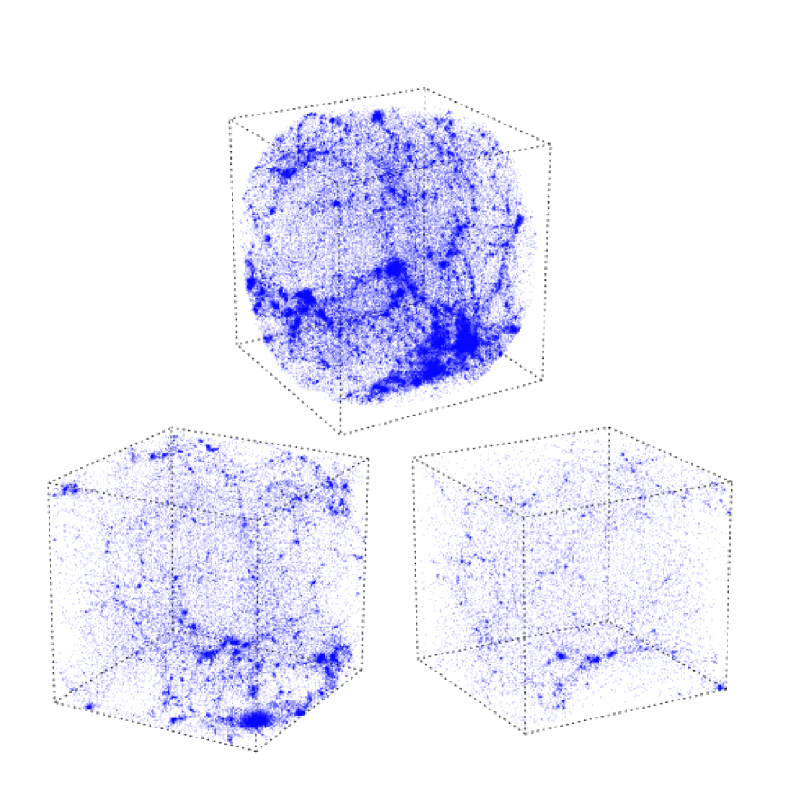
Figure 1: Spatial structure in a void-like region selected from an N-body simulation of structure formation in the SCDM scenario. Three consecutive zoom-ins centered on the core of the void are shown: a $45\hbox{Mpc}$ diameter particle sphere (top), $36\hbox{Mpc}$ (bottom left) and $30\hbox{Mpc}$ (bottom right). The existence of substructure within the void region is readily apparent, although it becomes more faint and tenuous towards the increasingly depleted interior of the void.

Nevertheless, in this study we show that the formation and evolution of foamlike patterns can indeed be described by the excursion set analysis. This is accomplished by focusing on the evolution of underdense regions, the voids, rather than overdensities in the matter distribution. Whereas much of the mass in the universe is bound-up in virialized structures, most of the volume is occupied by large underdense voids: voids are the dominant component of the Megaparsec-scale galaxy and matter distributions. In a void-based description of structure formation, matter is squeezed in between expanding voids, and sheets and filaments form at the intersections of the void walls (Icke 1984; Van de Weygaert 1991, 2002). Such a view is supported by Regős & Geller (1991), Dubinski et al. (1993) and Van de Weygaert & Van Kampen (1993), who give clear and lucid descriptions of how voids evolve in numerical simulations of gravitational clustering. We will stick to this basic framework in the present study.

We will argue that low density regions are the objects-of-choice for working out a succesful analytical description of cosmic spatial structure, if it is to be based upon the idealization of spherical symmetry. This is because, in many respects, voids are ideally suited for an excursion set analysis based on a spherical evolution model. This is despite the fact that voids form from negative density perturbations in the initial fluctuation field, and neither maxima nor minima in the primordial Gaussian field, are spherical (see Bardeen et al. 1986). However, in marked contrast to the evolution of density peaks, primordial asphericity of negative density perturbations is quickly lost as they expand: the generic evolution is towards an approximately spherical tophat geometry (Icke 1984). Moreover, the velocity structure of uniform density voids is simple to understand; an observer in the interior will observe a Hubble-type velocity field. All of this is discussed in some detail in Appendix A, which describes the evolution of a single isolated void.

Although the image of a large scale matter distribution organized by expanding voids is appealing, in its basic form, the description essentially involves an extrapolation of single void characteristics to an entire random population of strictly distinct and non-interacting peers, each of them undisturbed smoothly expanding bubbles. This discards one of the most crucial and characteristic aspects of cosmic structure formation—that there are no isolated voids, nor smoothly unstructured ones. Any complete analysis will have to take into account the complications which arise from

• the substructure present within the primordial volume occupied by the void, and

• the inhomogeneous matter distribution in its vicinity.

The existence of internal void structure is not unexpected. The void shown in Figure 1, selected from a large N-body simulation of cosmic structure formation, shows the existence of structure on all scales. The figure shows three successive zoom-ins on the inner parts of the void; all exhibit some measure of internal structure, although substructure is less pronounced in the emptiest inner regions.

As was mentioned above, all viable cosmological structure formation scenarios imply a hierarchical mode of structural growth. The formation of any object involves the fusion of all substructure present within its realm, including the small-scale objects which had condensed out at an earlier stage. Underdensities are organized similarly—in the evolution of a void we may identify two, intimately related, processes:

• a bottom-up assembly, in which a void emerges as a mature and well-defined entity through the fusion and gradual erasure of its internal substructure, and

• the interaction of the void with its surroundings, marking its participation in the continuing process of hierarchical structure formation.

Considerable insight into the evolution of voids came from the rigorous and insightful study by Dubinski et al. (1993). Following an analytical study of (isolated) spherically symmetric voids by Blumenthal et al. (1992), they used N-body simulations to study the evolution of the void hierarchy from a set of artificial and simplified initial conditions, consisting of various levels of hierarchically embedded spherical tophat voids. They showed that adjacent voids collide, producing thin walls and filaments as the matter between them is squeezed. Mainly confined to tangential motions, the peculiar velocities perpendicular to the void walls are mostly suppressed. The subsequent merging of voids is marked by the gradual fading of these structures while matter evacuates along the walls and filaments towards the enclosing boundary of the “void merger”. The timescale on which the internal substructure of a void is erased is approximately the same as that when the void itself approached “nonlinearity” (Appendix A gives a precise definition of what is meant by nonlinearity). At nonlinearity, smaller-scale voids collide and merge with one another, effectively dissolving their separate entities into one larger encompassing void. Only a faint and gradually fading imprint of their original outline remains as a reminder of the initial internal substructure. As this (re)arrangement of structure progresses to ever larger scales, the same basic processes repeat.

N-body simulations of voids evolving in more generic cosmological circumstances by Van de Weygaert & Van Kampen (1993) (also see Van de Weygaert 1991) yielded similar results. This prompted them to suggest the existence of a natural void hierarchy, in which small-scale voids embedded within a pronounced large-scale void gradually fade away. An illustration of such a void hierarchy process, within the context of the CDM scenario, is shown in Figure 2. The major characteristics of an evolving void hierarchy, the gradual blending of small-scale voids and structures into a larger surrounding underdensity, is clearly visible in the sequence of six timesteps.

However, the artificial arrangement of voids embedded within voids represents only one aspect of reality—it misses a crucial component of the development of a void hierarchy. An evolving void hierarchy not only involves the merging of small voids into larger voids, but also the disappearance of small voids as they become embedded in larger-scale overdensities. Thus, in contrast to the process of dark halo formation, the emerging void hierarchy is ruled by two processes instead of one. The main goal of this paper is to incorporate both processes into a model of the void hierarchy. We do this by combining the spherical evolution model with the excursion set approach. When used to describe the evolution of overdense clouds, the excursion approach requires consideration of a one-barrier problem, the single barrier representing what is required for collapse in the spherical evolution model. We show that the excursion set formulation of the void hierarchy requires consideration of two-barriers: one barrier is associated with the collapse of clouds, and the other with the formation of voids. The resulting framework is able to describe realistic settings of random density fields in which voids interact with their surroundings.

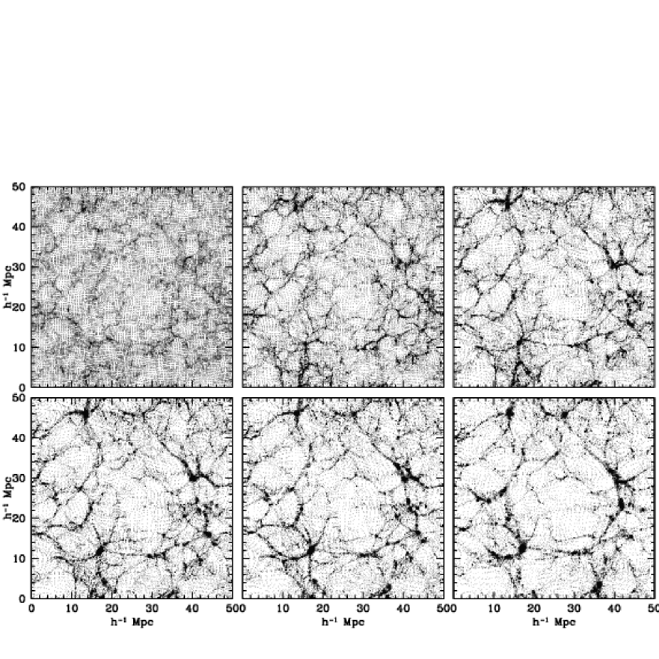
Figure 2: Void evolution. Six timesteps in the evolution of a void region in a 128³ particle N-body simulation of structure formation in an SCDM model: top-left to bottom-right shows expansion factors $a_{\rm exp}=0.1,0.2,0.3,0.35,0.4$ and $0.5$ (the present time has $a_{\rm exp}=1.0$). Initial conditions were defined such that they would focus in on a $3\sigma(4h^{-1}\hbox{Mpc})$ void, using a constrained random field code (Van de Weygaert & Bertschinger 1996). The sequence shows the gradual development of a large void of diameter $\approx 25h^{-1}\hbox{Mpc}$ as the complex pattern of smaller voids and structures which had emerged within it at an earlier time, merge with one another. This illustrates one aspect of the evolving void hierarchy: the void-in-void process.

This paper is organized as follows. Section 2 discusses important generic properties of isolated voids, which grow from depressions in the primordial density field, propelled by the perturbed gravitational field. The spherical model forms the core of further analytical considerations, and is discussed in some detail in Appendix A. Section 3 discusses the generic effects of larger scale stucture on the evolution of voids. Two crucial processes which shape the void hierarchy are described: the void-in-void mode and the void-in-cloud mode. How these processes can be incorporated into the excursion set approach using two-barriers is the subject of Section 4. Section 5 describes the associated distribution of void sizes, which is predicted to have a universal form, and to be peaked around a characteristic value. One of the results of Section 5 is to show that peak-based models should be reasonably accurate for the largest voids, but, because they account neither for the void-in-void mode nor for the void-in-cloud mode, they predict many more small voids than does the excursion set approach. Appendix B discusses the “basic troughs model”, which assumes there is a one-to-one identification between minima in the primordial Gaussian density field, with centres of voids in the evolved (and nonlinear) matter distribution. This also serves to define notation for the “adaptive troughs model” which is described in Section 5.1.

Section 6 presents various other aspects of the hierarchically evolving void population. Global parameters, such as the fraction of mass in the cosmos contained within void regions, along with the fraction of space occupied by voids, are readily derived from the void size distribution. In addition, the formalism is applied towards a reconstruction of the ancestral history of a given void, followed by an evaluation of the environmental influence on basic void properties. We also put forward suggestions towards an analytical treatment of the influence of the void environment on the galaxies that may form within. Finally, we indicate how an assessment of the evolution of dark matter clustering may be predicated on our formalism. In Section 7, we provide an overview of our results and seek to embed these in the wider context of the study of hierarchical structure formation. We also comment on how our results for the distribution of voids in the dark matter distribution may be related to observations of voids in the galaxy distribution. Although our model provides a useful framework, developing a more detailed model is beyond the scope of this work. The results of numerical studies of void galaxies in semi-analytic galaxy formation models are described by Mathis & White (2002) and Benson et al. (2003).

2 Evolution of isolated voids

The basic features of voids can be understood in terms of the evolution of isolated density depressions. The net density deficit brings about a sign reversal of the effective gravitational force: a void form from a region which induces an effective repulsive peculiar gravity.

Figure 3: Spherical model for the evolution of voids. Left: a pure (uncompensated) tophat void evolving up to the epoch of shell-crossing. Initial (linearly extrapolated) density deficit was $\Delta_{lin,0}=-10.0$, initial (comoving) radius ${\widetilde{R}}_{i,0}=5.0h^{-1}\hbox{Mpc}$. Timesteps: $a=0.05,0.1,0.2$ and $0.3$. Right: a void with an angular averaged SCDM profile (BBKS, eqn. 7.10). Initial density deficit and characteristic radius are same as for the tophat void (left). The tendency of this void to evolve into a tophat configuration by the time of shell crossing is clear. Shell-crossing, and the formation of an obvious ridge, happens only if the initial profile is sufficiently steep.

In physical coordinates, overdense regions expand slightly less rapidly than the background, reach a maximum size, and then turn around and finally collapse to vanishingly small size (this is strictly true only in an Einstein de-Sitter or closed Universe). In contrast, underdense regions will not turn around: they undergo simple expansion until matter from their interior overtakes the initially outer shells. The generic characteristics of these evolutionary paths may be best appreciated in terms of the evolution of isolated spherically symmetric density perturbations, either overdense or underdense, in an otherwise homogeneous and expanding background universe. These spherical models provide a key reference for understanding and interpreting more complex situations. As a result of the spherical symmetry, the problem is essentially one-dimensional, allowing a fully analytic treatment and solution, making the model easier to analyze, interpret and understand. The spherical model for the evolution of isolated voids is discussed in some detail in Appendix A.

The most basic and universal properties of evolving spherical voids are:

• Expansion: Voids expand, in contrast to overdense regions, which collapse.

• Evacuation: As they expand, the density within them decreases continuously. (To first order, the density decrease is a consequence of the redistribution of mass over the expanding volume. Density decrease from mass lost to the surrounding overdensities is a second order, nonlinear effect occuring only near the edges.)

• Spherical shape: Outward expansion makes voids evolve towards a spherical geometry.

• Tophat density profile: The effective “repulsion” of the matter interior to the void decreases with distance from the center, so the matter distribution evolves into a (reverse) “tophat”.

• “Super-Hubble” velocity field: Consistent with its (ultimate) homogeneous interior density distribution, the (peculiar) velocity field in voids has a constant “Hubble-like” interior velocity divergence. Thus, voids evolve into genuine “Super-Hubble Bubbles”.

• Suppressed structure growth: Density inhomogeneities in the interior are suppressed and, as the object begins to resemble an underdense universe, structure formation within it gets frozen-in.

• Boundary ridge: As matter from the interior accumulates near the boundary, a ridge develops around the void.

• Shell-crossing: The transition from a quasi-linear towards a mature non-linear stage which occurs as inner shells pass across outer shells.

Figure 3 illustrates these features. Both panels show the time evolution of the density deficit profile. Consider the panel on the left, which illustrates the development of an initial (uncompensated) tophat depression (a “tophat” void). The initial (linear) density deficit of the tophat was set to $\Delta_{lin,0}=-10$, and its (comoving) initial radius was ${\widetilde{R}}_{i,0}=5h^{-1}\hbox{Mpc}$. The evolving density profile bears out the charactertistic tendency of voids to expand, with mass streaming out from the interior, and hence for the density to continuously decrease in value (and approach emptiness, $\delta=-1.0$). Initially underdense regions are just expanding faster than the background and will never collapse (in an $\Omega\leq 1$ Universe). Notice that this model provides the most straightforward illustration of the formation of a ridge. Despite the absence of any such feature initially, the void clearly builds up a dense and compact bounding “wall”.

For comparison with the tophat void configuration on the left, the panel on the right of Figure 3 depicts the evolution of a void whose initial configuration is more representative of cosmological circumstances. Here, the initial profile is the radial-averaged density profile for a trough in a Gaussian random field of Cold Dark Matter density fluctuations. The analytical expression for this profile was worked out by BBKS [1986] (eq. 7.10), and the one example we show here concerns the radial profile for a density dip with average steepness, i.e. $x\equiv-\langle\nabla^{2}f\rangle/\sigma_{2}=-1$. The same qualitative aspects of void evolution can be recognized as in the case of a pure tophat void: the void expands, empties (to a near-empty configuration $\Delta=-1$ at the centre), and also develops a ridge at its boundary. Notice that the void profile evolves into a configuration which increasingly resembles that of a “tophat” void. We will make use of this generic evolution in what follows.

Looking from the inside out, one sees the interior shells expanding outward more rapidly than the outer shells. With a minimum density near the void’s centre, and density which increases gradually as one moves outward, the density deficit $|\Delta(r)|$ of the void decreases as a function of radius $r$. The outward directed peculiar acceleration is directly proportional to the integrated density deficit $\Delta(r,t)$ and therefore decreases with radius: inner shells are propelled outward at a higher rate so that the interior layers of the void move outward more rapidly. The inner matter starts to catch up with the outer shells, leading to a steepening of the density profile in the outer realms. Meanwhile, over a growing area of the void interior, the density distribution is rapidly flattening. This is a direct consequence of the outward expansion of the inner void layers: the “flat” part of the density distribution in the immediate vicinity of the dip gets “inflated” along with the void expansion.

The features summarized above, which are seen in the idealized setting of initially smooth spherically symmetric voids, are also seen in more generic, less symmetric cosmological circumstances, when substructure is also present. Figure 2 provides one illustration of the evolution of more realistic an complex underdensities. N-body simulation studies of objects like this one have concluded that the tophat spherical model represent a remarkably succesfull desciption of reality (e.g. Dubinski et al. 1993; Van de Weygaert & Van Kampen 1993). The evolution towards a spherical top hat, whatever the initial configuration, is in stark contrast to how overdensities evolve. As a generic overdensity collapses, it contracts along a sequence of increasingly anisotropic configurations. Contraction leads to a “deflation” and accompanying steepening of density gradients, while the infall of surrounding structures marks a decreasing domain over which the neglect of substructure is realistic.

In summary, it is apparent that the top hat spherical model not only provides a rather useful model for the evolution of isolated voids, but that it develops into an increasingly accurate representation of reality over an increasingly large fraction of the expanding volume of the void.

3 Effect of larger-scale structures

If we wish to use voids to understand the complex spatial patterns in the universe, we need a prescription for identifying the present-day cosmic voids, and for describing how voids interact with the large-scale structure which surrounds them.

3.1 Importance of shell-crossing

The generic property of ridge formation (e.g. Fig. 3) is suggestive, and Blumenthal et al. [1992] argued that the observed voids in the galaxy distribution should be identified with primordial underdensities that have only just reached shell-crossing. For a perfectly spherical void with a perfect tophat profile this happens exactly when the primordial density depression out of which the void developed would have reached a linearly extrapolated underdensity $\delta_{\rm v}$. For such voids, $\delta_{\rm v}$ is independent of mass scale: $\delta_{\rm v}=-2.81$ in an $\Omega_{0}=1$ Universe. This threshold value will play an important role in our model of how the void hierarchy evolves. For instance, Dubinski et al. [1993] used this characteristic density to estimate that shell-crossing voids constitute a population of approximately volume-filling domains for a substantial range of cosmological structure formation scenarios. By contrast, overdense primordial perturbations collapse and virialize—they shrink in comoving coordinates. The resulting picture is one in which the matter in the Universe accumulates in ever smaller collapsing overdensities – in sheets, filaments and clusters – whose spatial arrangement is dictated by the growing underdense expanses.

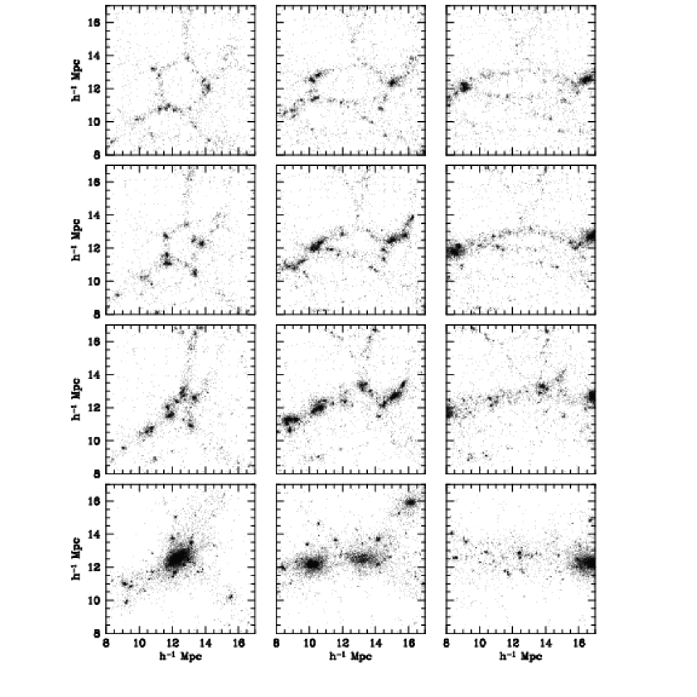
Figure 4: Three examples (left to right) of the void-in-cloud process in action in numerical simulations of structure formation in a SCDM scenario ($\Omega_{0}=1.0$, $h_{0}=0.5$). Top to bottom panels show the evolution of the particle distribution in comoving coordinates from early to late times (resp. $a=0.3,0.4,0.5$ and $1.0$, the current epoch). The initially underdense regions are crushed by the collapse of the overdense regions which surround them. The void in the first row of 4 panels shows a nearly spherical collapse sequence. The other two rows involve configurations involving more anisotropic surrounding matter distributions (and force fields).

3.2 Void Sociology

Two effects will seriously affect the number of small voids within a generic field of density perturbations. Both relate to the hierarchical embedding of a density depression within the larger scale environment.

First, consider a small region which was less dense than the critical $\delta_{\rm v}$. It may be that this region, which we would like identify as a void today, was embedded in a significantly larger underdense region which was also less dense than the critical density. Therefore, we would also like to identify the larger region as a large void today. Since many small voids may coexist within one larger void, we must not count all of the smaller voids as distinct objects, lest we overestimate the number of small voids, and the total volume fraction in voids. We will call this the void-in-void problem. It is analogous to the well-known cloud-in-cloud problem associated with the using the number density of initially overdense peaks to estimate the number of dense virialized clusters.

A second effect is responsible for a radical dissimilarity between void and halo populations: If a small scale minimum is embedded in a sufficiently high large scale maximum, then the collapse of the larger surrounding region will eventually squeeze the underdense region it surrounds; the small-scale void will vanish when the region around it has collapsed completely. If the void within the contracting overdensity has been squeezed to vanishingly small size it should no longer be counted as a void. Figure 4 shows three examples of this process, each identified from a large (SCDM) N-body simulation. To account for the impact of voids disappearing when embedded in collapsing regions, we must also deal with the void-in-cloud problem.

Virialized halos within voids are not likely to be torn apart as the void expands around them. Thus, the cloud-in-void phenomenon is irrelevant for dark halo formation. The asymmetry between the void-in-cloud and cloud-in-void processes effects a symmetry breaking between the emerging halo and void populations: although they evolve out of the same symmetric Gaussian initial conditions, we argue that over- and underdensities are expected to evolve naturally into agglomerations with rather different characteristics.

4 Excursion Formalism

In its simplest and most transparent formulation the excursion set formalism refers to the collapse of perfectly spherical overdensities, so this is the case which we will describe first.

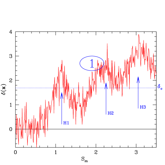
Figure 5: Excursion Set Formalism, illustrated for the formation of a halo. Random walk exhibited by the average overdensity $\delta$ centred on a randomly chosen position in a Gaussian random field, as a function of smoothing scale, parametrized by $S_{m}$ (large volume are on the left, small volumes on the right). Dashed horizontal line indicates the collapse barrier $\delta_{\rm c}$. The largest scale (smallest value of $S$) on which $\delta(S)$ exceeds $\delta_{\rm c}$ is an estimate of the mass of the halo which will form around that region.

4.1 Excursion set model of clusters

The jagged line in Fig. 5 represents the overdensity centred on a randomly chosen position in the initial Gaussian random field, as a function of the scale on which the overdensity was computed. The height of the walk $\delta_{0}(S)$ is the linear theory overdensity relative to the density of the background universe. The spatial scale is parametrized by its variance $S$ (defined in equation 61). In hierarchical models, $S$ decreases with increasing scale, so the largest spatial scales are on the left, and $\delta(S)\to 0$ as $S\to 0$. Because the initial fluctuations are small, the mass contained within the smoothing filter is $m\propto[1+(D_{i}/D_{0})\delta_{0}]\,R^{3}$, where $D_{i}$ denotes linear theory growth factor at the initial time. Since $D_{i}/D_{0}\ll 1$, $m\propto R^{3}$: the mass is proportional to the initial comoving scale cubed.

In the spherical collapse model, all regions with linear theory densities greater than $\delta_{\rm c}$ can have formed bound virialized objects, and this critical overdensity is independent of mass scale. This constant value is shown as the dashed line in same height at all $S_{m}$, where we have used the subscript $m$ to denote the fact that mass and initial scale are interchangeable. .

The excursion set formalism supposes that no mass can escape from a region which collapses. If $\delta_{0}=\delta_{\rm c}$ on scale $R$, then all the mass contained within $R$ is included in the collapsed object, even if $\delta_{0}<\delta_{\rm c}$ for all $r<R$. Thus, if the random walk height $\delta_{0}$ exceeds the value $\delta_{\rm c}$ after having travelled distance $S(R)$ it represents a collapsed object of mass $m\propto R^{3}$. A walk may cross the barrier $\delta_{\rm c}$ at many different values of $S(R)$. Each crossing corresponds to a different smoothing scale and, because $m\propto R^{3}$, contains a different amount of mass. However, of the various crossings of the barrier $\delta_{\rm c}$ the first crossing, at the smallest value of $S(R)$ for which $\delta_{0}\geq\delta_{\rm c}$, is special since it is this scale which is associated with the most mass. The crossings at smaller scales correspond to condensations of a smaller mass, which have been incorporated in the larger encompassing mass concentration.

In its simplest form, the excursion model for the distribution of masses of virialized objects equates the distribution of distances $S(R)$ which one-dimensional Brownian motion random walks, originating at the origin, travel before they first cross a barrier of constant height $\delta_{\rm c}$, with the fraction of mass which is bound up in objects of mass $m(R)$. The further a given walk travels before crossing the barrier, the smaller the mass of the object with which it is associated (Bond et al. 1991).

     

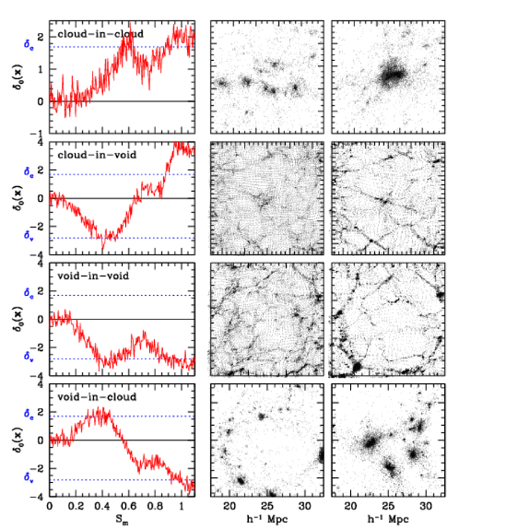
Figure 6: Four mode (extended) excursion set formalism. Each row illustrates one of the four basic modes of hierarchical clustering: the cloud-in-cloud process, cloud-in-void process, void-in-void process and void-in-cloud process (from top to bottom). Each mode is illustrated using three frames. Leftmost panels show ‘random walks’: the local density perturbation $\delta_{0}({\bf x})$ as a function of (mass) resolution scale $S_{m}$ (cf. Fig. 5) at an early time in an N-body simulation of cosmic structure formation. In each graph, the dashed horizontal lines indicate the collapse barrier $\delta_{\rm c}$ and the shell-crossing void barrier $\delta_{\rm v}$. The two frames on the right show how the associated particle distribution evolves. Whereas halos within voids may be observable (second row depicts a halo within a larger void), voids within collapsed halos are not (last row depicts a small void which will be squeezed to small size as the surrounding halo collapses). It is this fact which makes the calculation of void sizes qualitatively different from that usually used to estimate the mass function of collapsed halos.

4.2 Excursion set model of voids

In our discussion above of the halo mass function, we considered the cloud-in-cloud problem, and argued that the only cloud which should be counted was the largest possible one. To study voids in the excursion set approach one must first specify the boundary shape associated with the emergence of a void. This can be done if we know the critical underdensity $\delta_{\rm v}$ which defines a void, and in what follows we will use the epoch of shell-crossing, estimated using the spherical evolution model, to specify $\delta_{\rm v}$. Thus, $\delta_{\rm v}=-2.81$, independent of smoothing scale (as was $\delta_{\rm c}$).

One might have thought that whereas clusters form from overdensities, voids form from underdensities, so the distribution of voids can be estimated analogously to how one estimates the distribution of clusters — one simply replaces the barrier $\delta_{\rm c}$ with one at $\delta_{\rm v}$, and then studies the distribution of first crossings of $\delta_{\rm v}$. Thus, if the random walk $\delta_{0}$ first drops below the value $\delta_{\rm v}$ after having travelled distance $S(R)$ it represents a void of mass $m\propto R^{3}$ and physical size ${\cal R}\approx 1.7R$.

However, we have seen that we must be more careful; in addition to avoiding the double counting associated with the void-in-void process, we must also account for the void-in-cloud process. The strength of the excursion set formulation is that is shows clearly how to do this. Figure 6 illustrates the argument. There are four sets of panels. The left-most of each set shows the random walk associated with the initial particle distribution. The two other panels show how the same particles are distributed at two later times. The first set illustrates the cloud-in-cloud process. The mass which makes up the final object (far right) is given by finding that scale within which the linear theory variance has value $S=0.55$. This mass came from the mergers of the smaller clumps, which themselves had formed at earlier times (centre panel). If we were to center the random walk path on one of these small clumps, it would cross the higher barrier $\delta_{\rm c}/D(t)>\delta_{\rm c}$ at $S>0.55$, the value of $D(t)$ representing the linear theory growth factor at the earlier time $t$.

The second series of panels shows the cloud-in-void process. Here, a low mass clump ($S>0.85$) virializes at some early time. This clump is embedded in a region which is destined to become a void. The larger void region around it actually becomes a bona-fide void only at the present time, at which time it contains significantly more mass ($S=0.4$) than is contained in the low mass clump at its centre. Notice that the cloud within the void was not destroyed by the formation of the void; indeed, its mass increased slightly from $S>0.85$ to $S\sim 0.85$. Such a random walk is a bona-fide representative of $S\sim 0.85$ halos; for estimating halo abundances, the presence of a barrier at $\delta_{\rm v}$ is irrelevant. On the other hand, walks such as this one allow us to make some important inferences about the properties of void-galaxies, which we will discuss shortly.

The third series of panels shows the formation of a large void by the mergers of smaller voids: the void-in-void process. The associated random walk looks very much the inverse of that for the cloud-in-cloud process associated with halo mergers. The associated random walk shows that the void contains more mass at the present time ($S\sim 0.4$) than it did in the past ($S>0.4$); it is a bona-fide representative of voids of mass $S\sim 0.4$. A random walk path centered on one of these mass elements which make up the filaments within the large void would resemble the cloud-in-void walk shown in the second series of panels. [Note that the height of the barrier associated with voids which are identified at cosmic epoch $t$ scales similarly to the barrier height associated with halo formation: $\delta_{\rm v}(t)\equiv\delta_{\rm v}/D(t)$.]

Finally, the fourth series of panels illustrates the void-in-cloud process. The particle distribution shows a relatively large void at the early time being squeezed to a much smaller size as the ring of objects around it collapses. A simple inversion of the cloud-in-void argument would have tempted one to count the void as a relatively large object containing mass $S\sim 1$. That this is incorrect can be seen from the fact that, if we were counting halos, we would have counted this as a cloud containing significantly more mass ($S\sim 0.3$), and it does not make sense for a massive virialized halo to host a large void inside.

Thus, the excursion set model for voids which we will develop below is as follows: If a walk first crosses $\delta_{\rm c}$ and then crosses $\delta_{\rm v}$ on a smaller scale, then the smaller void is contained within a larger collapsed region. Since the larger region has collapsed, the smaller void within it no longer exists, so it should not be counted. The only bona-fide voids are those associated with walks which cross $\delta_{\rm v}$ without first crossing $\delta_{\rm c}$. The problem of estimating the fraction of mass in voids reduces to estimating the fraction of random walks which first crossed $\delta_{\rm v}$ at $S$, and which did not cross $\delta_{\rm c}$ at any $S^{\prime}<S$. Thus, a description of the void hierarchy requires solution of a two-barrier problem.

Clearly, the model predictions will depend on $\delta_{\rm c}$ and $\delta_{\rm v}$. If we use the spherical tophat model summarized in Appendix A to set these values, then it seems reasonable to set $\delta_{\rm v}=-2.81$. But how we account for the void-in-cloud problem is somewhat more subtle. Suppose we choose $\delta_{\rm c}=1.686$, the value associated with complete collapse. In effect, this allows a void to have the maximum possible size it can have, given its underdensity, unless it is within a fully collapsed halo, in which case it has zero size. Presumably, if it is within a collapsing region which has not yet collapsed completely (as in the bottom-right panel of Figure 6), then its size is intermediate between the size one would have estimated from the isolated spherical evolution model, and zero. Thus, only excluding voids in regions which have collapsed completely almost certainly overestimates the typical void size (furthermore, we are ignoring the thickness of the ridge around each void). Another natural choice is $\delta_{\rm ta}=1.06$; this ignores all voids that are within regions which are beginning to turnaround, even though they may still have non-neglibigle sizes, and so underestimates the abundance of large voids. Accounting more carefully for the effect of the void-in-cloud problem is the subject of ongoing work.

In summary, what distinguishes voids from collapsed objects is the following: Whereas it may be possible to have a cluster within a void it does not make physical sense to have a void within a cluster. The excursion set formulation allows one to account for this.

5 Universal Void Size Distribution

Let ${\cal F}(S,\delta_{\rm v},\delta_{\rm c})$ denote the fraction of walks which first cross $\delta_{\rm v}$ at $S$, and which do not cross $\delta_{\rm c}$ until after they have crossed $\delta_{\rm v}$ (i.e., if they cross $\delta_{\rm c}$, they do so at $s\geq S$). Then ${\cal F}(S,\delta_{\rm v},\delta_{\rm c})$ is the distribution of first crossings of the type associated with voids. Appendix C shows that this first crossing distribution is given by

$$S\,{\cal F}(S,\delta_{\rm v},\delta_{\rm c}) = \sum_{j=1}^{\infty}{j^{2}\pi^{2}{\cal D}^{2}\over\delta_{\rm v}^{2}/S}\,{\sin(j\pi{\cal D})\over j\pi},$$ (1)

$$\qquad\times\exp\left(-{j^{2}\pi^{2}{\cal D}^{2}\over 2\,\delta_{\rm v}^{2}/S}\right),$$

where

$${\cal D}\equiv{|\delta_{\rm v}|\over(\delta_{\rm c}+|\delta_{\rm v}|)}\,.$$ (2)

In an Einstein de-Sitter universe, $\delta_{\rm c}$, $\delta_{\rm v}$ and $\sigma(m)$ all have the same time dependence, so equation (1) evolves self-similarly. In more general world-models the time dependences only slightly different, so the approximation of self-similar evolution should be quite accurate.

The quantity ${\cal D}$ is the “void-and-cloud parameter”; it parameterizes the impact of halo evolution on the evolving population of voids. To see why, notice that the likelihood of smaller voids being crushed through the void-in-cloud process decreases as the relative value of the collapse barrier $\delta_{\rm c}$ with respect to the void barrier $\delta_{\rm v}$ becomes larger.

This is also consistent with the fact that

$$\int{\cal F}(S,\delta_{\rm v},\delta_{\rm c})=1-{\cal D}={\delta_{\rm c}\over\delta_{\rm c}+|\delta_{\rm v}|},$$ (3)

(e.g., equation 77) represents the mass fraction in voids. Thus, if ${\cal D}$ is small, voids account for nearly all the mass. On the other hand, for any noticeable impact of the void-in-cloud process the mass fraction in voids, $1-{\cal D}$, will be less than unity. The more important the void-in-cloud process is, the smaller the mass fraction in voids will be, as more voids are squeezed to vanishingly small size.

Relation (7) suggests that the volume fraction in voids is $1.7^{3}\,(1-{\cal D})$. For $\delta_{\rm v}=-2.81$ and $\delta_{\rm c}=1.686$, this ratio is larger than unity, indicating that the voids fill the universe. (The volume fraction in voids is also larger than unity if we set $\delta_{\rm c}=1.06$ instead.) Thus, we have a model in which about one third of the mass of the universe is associated with voids which occupy most of the volume. The remaining seventy percent of the mass is in between the voids, and occupies negligible volume.

Although the sum in equation (1) converges reasonably rapidly, it is not so easy to see what shape it implies. We have found that equation (1) is quite well approximated by

$$\nu f(\nu)\approx\sqrt{\nu\over 2\pi}\,\exp\left(-{\nu\over 2}\right)\,\exp\left(-{|\delta_{\rm v}|\over\delta_{\rm c}}\,{{\cal D}^{2}\over 4\nu}-2{{\cal D}^{4}\over\nu^{2}}\right),$$ (4)

where we have set

$$\nu\,\equiv\,\delta_{\rm v}^{2}/S\equiv\,\delta_{\rm v}^{2}/\sigma^{2}(m)\,,$$ (5)

and $\nu f(\nu)\,{\rm d}\nu/\nu=S{\cal F}(S)\,{\rm d}S/S$. (This expression is accurate for values of $\delta_{\rm c}/|\delta_{\rm v}|\geq 1/4$ or so.) Expression (4) shows clearly that $f(\nu)$ cuts-off sharply at both small and large values of $\nu$. In other words, the distribution of void masses is reasonably well peaked about $\nu\approx 1$, corresponding to a characteristic mass of order $\sigma_{0}(m)\approx|\delta_{\rm v}|$.

When $\delta_{\rm c}\gg|\delta_{\rm v}|$, then ${\cal D}\to 0$, and the second exponential tends to unity. In this limit, the two-barrier distribution reduces to that associated with a single barrier at $\delta_{\rm v}$. This shows explicitly that when the void-in-cloud process is unimportant (${\cal D}\to 0$), then the abundance of voids is given by accounting correctly for the void-in-void process.

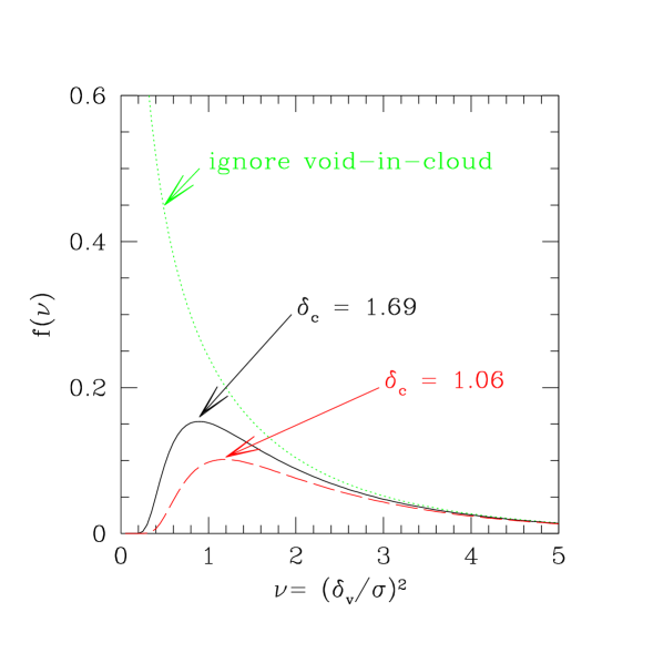
Figure 7: Scaled distribution of void masses/sizes: voids which enclose large masses have large values of $\nu$. Curves show equation (1) with $\delta_{\rm v}=-2.81$ and two choices of $\delta_{\rm c}$ as labeled. These choices are motivated by the spherical collapse model, and result in a distribution which is well peaked about a characteristic value. Ignoring the void-in-cloud process altogether is equivalent to setting $\delta_{\rm c}\to\infty$. Although decreasing $\delta_{\rm c}/|\delta_{\rm v}|$ decreases the abundance of low mass halos, the abundances of voids which enclose the most mass are not sensitive to the value of $\delta_{\rm c}$.

Figure 7 illustrates the resulting void size distributions. Notice that the mass fraction in small voids depends strongly on $\delta_{\rm c}$ (the divergence at low $\nu$ associated with the void-in-void solution is removed as $\delta_{\rm c}$ increases), whereas the mass fraction enclosed by the largest voids depends only on $\delta_{\rm v}$. This is primarily a consequence of the fact that large underdensities embedded in a larger region of average density are rare, so such regions embedded in large overdensities are rarer still. Since there are essentially no large-scale underdensities embedded in larger scale overdensities, on scales where $\sigma\ll(\delta_{\rm c}+|\delta_{\rm v}|)$, the value of $\delta_{\rm c}$ is irrelevant. Thus, the distribution of large voids is almost exclusively determined by $\delta_{\rm v}$. We will return to this shortly.

The number density $n(m)$ of voids which contain mass $m$ is obtained by inserting expression (1) in the relation

$${m^{2}\,n_{\rm v}(m)\over\bar{\rho}}=S\,{\cal F}(S,\delta_{\rm v},\delta_{\rm c})\,{{\rm d\ ln}\,S\over{\rm d\ ln}\,m}.$$ (6)

To illustrate what our two-barrier model implies for void sizes, we must convert the expression above for the fraction of mass in voids to a void-size distribution. The simplest approximation, motivated by the spherical tophat void model, sets the comoving volume $v$ of the void equal to

$$v=(m/\bar{\rho})\times 1.7^{3}\,.$$ (7)

Since all the time dependence enters via $\nu=\delta^{2}_{\rm v}(z)/\sigma^{2}(m)$, the distribution of void sizes evolves self-similarly. Simple changes of variables relate the void volume or mass functions to the barrier crossing distribution: $f(v){\rm d}v=f(m){\rm d}m=f(\nu){\rm d}\nu$.

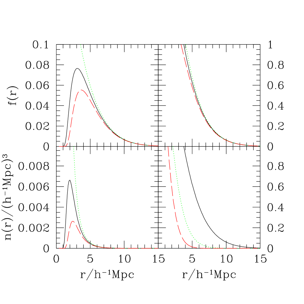
Figure 8: Distribution of void radii predicted by equation (4), in an Einstein de-Sitter model with $P(k)\propto k^{-1.5}$, normalized to $\sigma_{8}=0.9$ at $z=0$. Top left panel shows the mass fraction in voids of radius $r$. Bottom left panel shows the number density of voids of radius $r$. Note that the void-size distribution is well peaked about a characteristic size provided one accounts for the void-in-cloud process. Top right panel shows the cumulative distribution of the void volume fraction. Dashed and solid curves in the top panels and bottom left panel show the two natural choices for the importance of the void-in-cloud process discussed in the text: $\delta_{\rm c}=1.06$ and 1.686, with $\delta_{\rm v}=-2.81$. Dotted curve shows the result of ignoring the void-in-cloud process entirely. Clearly, the number of small voids decreases as the ratio of $\delta_{\rm c}/|\delta_{\rm v}|$ decreases. Bottom right panel shows the evolution of the cumulative void volume fraction distribution. The three curves in this panel are for $\delta_{\rm c}=1.686(1+z)$, where $z=0$ (solid), 0.5 (dotted) and 1 (dashed).

As a specific illustration of what our model implies, Fig. 8 shows the distribution of void sizes in a model where the initial power-spectrum was $P(k)\propto k^{n}$ with $n=-1.5$, normalized so that the rms fluctuations in a tophat sphere of radius unity was $\sigma_{8}=0.9$ at $z=0$. The top left panel shows the mass fraction in voids of radius $r$, and the bottom left panel shows the number density of such voids. The three curves in each panel show equation (4) with $\delta_{\rm c}=1.06$, 1.686 and $\infty$, and we have set $\delta_{\rm v}=-2.81$ in all cases. Notice how the abundance of small voids decreases dramatically as the ratio $\delta_{\rm c}/|\delta_{\rm v}|$ decreases. By contrast, the abundance of large-scale voids is largely insensitive to this ratio (also see Fig. 7).

We can make a rough estimate of the scale of the peak by computing that $\nu$ at which equation (4) is maximized. This requires solution of a cubic, and gives $\nu_{\rm max}$ decreasing as ${\cal D}$ decreases. For the range of $0.6\leq{\cal D}\leq 0.75$ of interest, it is usually close to unity: $\nu_{\rm max}\approx 1$. To estimate the typical void size we will therefore simply use the approximate value of $\sigma\sim|\delta_{\rm v}|$.

For a power spectrum approximated by a power-law of slope $n$, the initial comoving size $R_{i}$ of a region which is identifed as a void is,

$${|\delta_{\rm v}|\over\sigma_{8}}=\left({8\over R_{\rm i}}\right)^{(n+3)/2}\quad\Rightarrow\quad R_{\rm i}=8\,\left({\sigma_{8}\over|\delta_{\rm v}|}\right)^{2/(n+3)}\,$$ (8)

with $\sigma_{8}$ denoting the rms fluctuation on scales of $8h^{-1}$Mpc (currently favoured $\Lambda$CDM models have $\sigma_{8}\approx 0.9$). This means that the final size $r_{v}$ of the void is

$${r_{v}\over h^{-1}{\rm Mpc}}\sim 1.7\times{8\over 3^{2/(3+n)}}\,\left({\sigma_{8}\over 0.9}{2.7\over|\delta_{\rm v}|}\right)^{2/(3+n)}.$$ (9)

A reasonable approximation to CDM spectra on Megaparsec scales is obtained by setting $n=-1.5$. In this case, the typical void radius is $\sim 3h^{-1}$Mpc. Since the correlation length is of order $8h^{-1}$Mpc, this makes the typical void diameter of order the correlation length.

The top right panel shows the cumulative distribution of the volume fraction for the three choices of $\delta_{\rm c}$. In all three cases, voids with radii greater than $5h^{-1}$ account for about sixty percent of the volume. This suggests that, for sufficiently large voids, the details of the void-in-cloud process are not important. It is easy to see why: a typical cluster forms from a region which had comoving radius $R_{i}\sim 8\,(\sigma_{8}/\delta_{\rm c})^{2/(3+n)}\sim 3.5h^{-1}$Mpc. Since few collapsing regions are larger than this, voids which are initially larger than this are extremely unlikely to have been squeezed out of existence.

Finally we turn to an estimate of how the volume fraction in voids evolves in this model. Since $\sigma_{8}(z)=\sigma_{8}/(1+z)$, the typical comoving size of voids is expected to be smaller at higher redshifts, by a factor of $(1+z)^{-2/(3+n)}$. The bottom panel shows the cumulative distribution at redshifts zero, one-half and unity (solid, dotted and dashed curves) where we have approximated $\delta_{\rm c}(z)\,=\,1.686(1+z)$ and $\delta_{\rm v}(z)=-2.81(1+z)$.

5.1 Alternative Models

To better appreciate the ramifications of the two-barrier excursion set model, it is instructive to explore alternative descriptions. This section discusses two models which follow from associating present-day voids with sufficiently underdense troughs in the initial fluctuation field.

5.1.1 The Basic Troughs Model

The most straightforward model of the void distribution is to suppose that voids are associated with minima in the initial density field. The simplest approximation to the number density of voids comes from smoothing the initial density fluctuation field with a filter of scale $R$, and then counting the number of minima of depth $\delta_{\rm v}$ in the smoothed field. If one assumes that all the initial minima survive to the present time, then the number density of minima gives the number density of voids. BBKS [1986] show that the density of minima of depth

$$\nu\ =\ {\displaystyle\delta^{2}_{\rm v}\over\displaystyle\sigma^{2}_{0}(m)}\,,$$ (10)

in a Gaussian random field is

$$n_{\rm v}(\nu)\,{\rm d}\nu=\sqrt{\nu\over 2\pi}\,{\exp(-\nu/2)\over(2\pi)^{3/2}R_{*}^{3}}\,{G(\gamma,\gamma\nu^{1/2})\over 2}\,{{\rm d}\nu\over\nu},$$ (11)

where the spectral parameters $R_{*}$ and $\gamma$ depend on the shape of the power spectrum of the initial density fluctuation field, whose definition is given in Appendix B, along with that of the integral expression for the function $G(\gamma,\gamma\nu^{1/2})$. (Strictly speaking, BBKS considered density maxima rather than minima. However Gaussian fluctuations are symmetric around the mean, so the density of peaks and troughs of the same absolute height is the same.)

Notice that, in this model, the abundance of density minima in the primordial Universe depends on the depth of the minimum. If we define

$$f(\nu)\,{\rm d}\nu\equiv(m/\bar{\rho})\,n_{\rm v}(\nu)\,{\rm d}\nu$$

and use the fact that the mass under a Gaussian filter is

$$m\,=\,{\bar{\rho}}\,(2\pi)^{3/2}R^{3}\,,$$ (12)

then we have a quantity which one might interpret as the fraction of mass which is in minima of depth $\nu$. Unfortunately, for a comparison with the distribution of void sizes, this is a rather awkward quantity, since, in this picture, all voids contain the same mass $m$ whatever their height $\nu$ (because the smoothing radius $R$ is the same for all the voids).

However, intuitively one would expect that deeper primordial minima should be identified with voids containing more mass, something which the above expression does not accomplish self-consistently. The model discussed in the next subsection attempts to account for the correlation between void mass and depth.

5.1.2 An Adaptive Troughs Model

If, instead, we smooth the initial density field with a range of filter sizes $R$, and identify voids with minima of depth $\delta_{\rm v}/\sigma_{0}(m)$, then, because $\sigma_{0}$ decreases as $R\propto m^{1/3}$ increases, we have a model in which voids which contain more mass are associated with deeper minima. Appel & Jones [1990] show how the changing smoothing scale modifies equation (11). The abundance of voids one obtains by replacing the BBKS [1986] formula (our equation 11) with the one given by Appel & Jones [1990] is

$$\nu f(\nu)=\sqrt{\nu\over 2\pi}{\exp(-\nu/2)\over 3\,(R_{*}/R)^{3}}{H(\gamma,\gamma\nu^{1/2})\over\gamma\nu^{1/2}}{R^{2}\sigma_{1}^{2}(R)\over\sigma_{0}^{2}(R)}\,{{\rm d}m/m\over{\rm d}\nu/\nu},$$ (13)

in which we have set $m/\bar{\rho}=(2\pi)^{3/2}R^{3}$, the relation between mass and filter radius for a Gaussian smoothing filter, $\gamma$ is defined in equation (67), and

$$H(\gamma,y)=\int_{0}^{\infty}{\rm d}x\,xf(x)\,{\exp[-(x-y)^{2}/2(1-\gamma^{2})]\over\sqrt{2\pi(1-\gamma^{2})}},$$

where $f(x)$ is given in equation (B.1), At large $\nu$ (i.e., for deep minima), $H\approx\gamma\nu^{1/2}\,G$, where $G$ is defined in Appendix B.1, so this expression is the same as equation (11). The two expressions differ significantly at smaller $\nu$. If the initial spectrum of density fluctuations was a power law, $P(k)\propto k^{n}$, then equation (13) for the void mass function becomes

$$\nu f(\nu)=\sqrt{\nu\over 2\pi}\exp\left(-{\nu\over 2}\right){H(\gamma,\gamma\nu^{1/2})\over 2\ \gamma\nu^{1/2}}\left({5+n\over 6}\right)^{3/2},$$ (14)

where we have used the fact that, for a Gaussian filter, $\gamma^{2}=(n+3)/(n+5)$, and $(R/R_{*})^{2}=(n+5)/6$. Comparison with the excursion set approximation (equation 4) shows that both estimates contain the term $\sqrt{\nu/2\pi}\exp(-\nu/2)$, responsible for the exponential cut-off at large sizes. However, the additional correction factors differ substantially. For instance, in contrast to the excursion set formula, the correction factor in this primordial troughs model explicitly depends on the shape of the initial power spectrum.

Although the distribution of void sizes associated with equation (13) cuts off exponentially at large sizes, as does the excursion set formula, it diverges at small sizes:

$$n(m)\,\propto\,m^{-2}.$$ (15)

Since this peaks model ignores both the void-in-void and the void-in-cloud processes, the divergence towards small void sizes is likely to be a significant overestimate. However, the large scale cut-off is likely to be accurate, probably even more-so than the excursion-set approximation (see below).

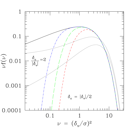
Figure 9: Scaled distribution of void masses/sizes (equation 1): voids which contain large masses have large values of $\nu$. Ignoring the void-in-cloud process entirely yields the upper most curve. The spherical evolution model suggests $\delta_{\rm c}\approx|\delta_{\rm v}|/2$; in this case, the void distribution is reasonably well peaked about a characteristic value. Lower and upper dotted lines which extend to small values of $\nu$ show predictions derived from equations (11) and (13) of the peaks model. These predictions depend on the shape of the initial power spectrum: curves assume $P(k)\propto k^{-1.5}$.

For comparison, the lower and upper dotted curves in Fig. 9 show the two predictions associated with these primordial troughs models: equations (11) and (13). These predictions depend on the shape of the initial power spectrum, and for the curves in Fig. 9 we have assumed $P(k)\propto k^{-1.5}$. The contrast between the small scale divergence of the peak/troughs formulae, with the small scale cut-off for the excursion set distributions, is obvious. Notice that the peaks/troughs models predict systematically more very large voids than does the excursion set model. The reason for this is closely related to the fact that the excursion set model does not include a factor like that in equation (8) of Appel & Jones [1990]. For this reason, at large $\nu$, the peaks–based model is likely to be more accurate.

5.2 Void distribution and spatial patterns

Our extension of the excursion set formalism provides a useful framework within which to construct an understanding of the dichotomy between the overdense and underdense regions of space in any hierarchical structure formation scenario.

Because voids occupy most of the volume, the peaked void distribution predicted by our excursion analysis has strong implications for the expected spatial patterns in the cosmic matter distribution. Since the sizes of most voids will be similar to the characteristic void size, our findings suggest that the cosmic matter distribution will resemble a foamlike packing of spherical voids of similar size and excess expansion rate. The dynamical origin of such a matter distribution had been recognized by various authors, in particular within the context of analyses based upon an extrapolation of the Zel’dovich approximation (see Shandarin & Zel’dovich 1989) and its extension, the adhesion approximation (Kofman, Pogosyan & Shandarin 1990). The role of voids in the latter had indeed been recognized by Sahni, Sathyaprakash & Shandarin (1994). These studies spurred the concepts of a cosmic web or cosmic skeleton (see e.g. Van de Weygaert 1991, Bond, Kofman & Pogosyan 1996, Novikov, Colombi & Doré 2003). Such patterns are naturally expected for cosmological scenarios with a lowpass power spectrum, characterized by a sharp spectral cutoff, as they would imply the imprint of an intrinsically dominating spatial scale. The four mode excursion formalism demonstrates and explains why the presence of such patterns is the natural outcome for a considerably wider range of Gaussian structure formation models.

As an interesting thought experiment, suppose we extrapolate our findings to an ultimate and asymptotic extreme: What if we approximate the “peaked” void distribution by a “spiked” distribution centered on the characteristic void size? In such a scenario, the cosmic matter distribution would be organized by a population of equally sized, spherical voids, all expanding at the same rate, akin to the scenario suggested by Icke [1984]. In this idealization, the walls and filaments would be found precisely at the midplanes between expanding voids, and the resulting skeleton of the matter distribution would be precisely that of a Voronoi Tessellation (Voronoi 1908; Okabe et al. 2000 and references therein). Our results appear to offer an explanation for the fact that heuristic models, based upon the use of tessellations as spatial templates for the galaxy distribution, can succesfully reproduce a variety of galaxy clustering properties (Van de Weygaert & Icke 1989; Van de Weygaert 1991; Goldwirth et al. 1995).

6 The Void Hierarchy

The void distribution function derived in the previous section allows us to study in some detail the processes involved in the formation and development of void-dominated patterns in the cosmic matter distribution. We have already discussed such gross features as the void-filling factor, and the mass fraction in voids. But the excursion set analysis paves the way to a detailed assessment of the temporal dependence of a particular void, on its “ancestral” heritage as well as its spatial dependence on environmental factors. The following subsections touch upon a few of these elements of void evolution.

6.1 Void mass and volume fractions

We have already argued that, in an Einstein de-Sitter universe, the mass fraction in voids does not evolve: approximately one-third of the mass is in voids (equation 3), and that these voids fill space. This conclusion does not depend strongly on cosmological model. Because the collapse barrier $\delta_{\rm v}(a)$ decreases with time, the typical comoving void radius is larger at late times. Therefore, the mass contained within a typical void is larger at late times. On the other hand, the total mass fraction does not evolve, from which we infer that the small mass voids present at early times must merge with each other to make the more massive voids which are present at later times.

6.2 Void ancestry

The mass contained in a void at the present time was previously partitioned up among many smaller voids, each separated by their own walls. This distribution can be estimated similarly to how Bond et al. [1991] and Lacey & Cole [1993] estimate the growth of clusters.

Consider a void $V_{0}$ which contains mass $M$ at a time $a_{0}$ when the critical densities for spherical collapse turnaround and void shell-crossing are $\delta_{\rm c0}$ and $\delta_{\rm v0}$, respectively. At an earlier epoch $a_{1}$, the critical densities were $\delta_{\rm c1}>\delta_{\rm c0}$ and $|\delta_{\rm v1}|>|\delta_{\rm v0}|$. The fraction of $M$ which was previously in voids that contained mass $m$ at the earlier time $a_{1}$ is given by inserting

$$\delta_{\rm c}\to\delta_{\rm c1}-\delta_{\rm v0};\quad\delta_{\rm v}\to\delta_{\rm v1}-\delta_{\rm v0};\quad S\to S(m)-S(M)$$ (16)

in equation (1). Integrating this over all possible ancestral voids (i.e., integrate over all $0<m\leq M$), yields the mass fraction of $M$ which was in voids at the earlier epoch also:

$$f_{\rm void}(M)\,=\,1\,+\,\left(\delta_{\rm v1}-\delta_{\rm v0}\over\delta_{\rm c1}-\delta_{\rm v1}\right)\,=\,{\delta_{\rm c1}-\delta_{\rm v0}\over\delta_{\rm c1}-\delta_{\rm v1}}\,.$$ (17)

Note how similar this expression is to the universal mass fraction in voids given by equation (3). Note in particular that this fraction is less than unity. This reflects the fact that, at earlier times, some of the mass currently affiliated with the void $V_{0}$ was not part of the ancestral voids. Instead, this fraction of its matter content resided in the walls (and filaments) which partitioned $V_{0}$ into its many smaller constituent voids. In an Einstein–de-Sitter universe

$$\delta_{\rm c1}-\delta_{\rm c0} = \delta_{\rm c0}\,(z_{1}-z_{0}),\quad{\rm and}$$

$$\delta_{\rm v1}-\delta_{\rm v0} = \delta_{\rm v0}\,(z_{1}-z_{0})\,,$$ (18)

so that the mass fraction of void matter which was in voids at the earlier time also is

$$f_{\rm void}(M)\,=\,1\,-\,{\cal D}_{0}\,{z_{1}-z_{0}\over(1+z_{1})}\,,$$ (19)

where ${\cal D}_{0}\equiv|\delta_{\rm v0}|/(\delta_{\rm c0}-\delta_{\rm v0})$ is the void-and-cloud parameter at the current epoch. Thus, at $z_{1}\approx z_{0}$, this fraction is close to unity, whereas for large lookback times $z_{1}\gg z_{0}$ it tends to $1-{\cal D}_{0}$ which is equal to the global void mass fraction (equation 3). In other words, the large voids emerging nowadays are to be traced back to an approximately average cosmic volume at early times.

The transformations above allow one to write down the excursion set predictions for the rate at which smaller voids merge to make bigger ones. The calculation is analogous to the one used when estimating the merger rates of collapsed halos, and we will leave it for future work. In other words, one may reconstruct the ancestry of voids, the void merger tree, although this exercise will be complicated by the high rate of premature void mortality.

6.3 Environmental Dependence

Suppose we evaluate the density field smoothed on a grid with cells of size $R$. The smoothed density will fluctuate from cell to cell. In the excursion set approach, we find that voids in denser cells 1) are smaller, 2) have a narrower size distribution, and 3) account for a smaller fraction of total mass in the cell they inhabit. This subsection quantifies these trends of “void bias”.

Consider a cell of size $V$ within which the density is $\bar{\rho}(1+\delta)$; i.e., this cell contains mass $M=\bar{\rho}V(1+\delta)$. In the spherical evolution model, the initial and final densities are related:

$$\delta_{0}(\delta)\!\!\! = \!\!\!{\delta_{\rm sc}\over 1.68647}\times\Biggl{[}1.68647-{1.35\over(1+\delta)^{2/3}}$$ (20)

$$\qquad\qquad\quad-{1.12431\over(1+\delta)^{1/2}}+{0.78785\over(1+\delta)^{0.58661}}\Biggr{]}$$

(e.g. Mo & White 1996). Note that $\delta_{0}$ has the same sign as $\delta$; initially dense regions become denser, whereas the comoving density in underdense regions decreases with time.

In the context of the void model studied here, voids which are in cells of volume $V$ within which the overdensity is $\delta$ are described by random walks which do not start from the origin $[S=0,\delta_{0}=0]$, but from the position $[S(M),\delta_{0}(\delta)]$. Therefore the fraction of the total mass $M=\bar{\rho}V(1+\delta)$ which is in voids of mass $m$ is given by setting

$$\delta_{\rm c} \to \delta_{\rm c}-\delta_{0}({\delta}),\qquad\delta_{\rm v}\to\delta_{\rm v}-\delta_{0}({\delta})$$

$$S \to S(m)-S\Bigl{[}\bar{\rho}V(1+\delta)\Bigr{]}$$ (21)

in equation (1). Integrating the resulting distribution over $0\leq m\leq M$ yields the fraction of mass, in a region of volume $V$ within which the density is $\delta$, which is contained in voids:

$$f_{\rm void}(\delta)\,=\,{\delta_{\rm c}-\delta_{0}(\delta)\over\delta_{\rm c}-\delta_{\rm v}}\,.$$ (22)

This indicates that the mass fraction $f_{\rm void}(\delta)$ decreases as the density $\delta$ of the cell increases. Conversely, as $\delta\to-0.8$, the density we associate with a void, then $\delta_{0}(\delta)\to\delta_{\rm v}$, and so $f_{\rm void}(\delta)\to 1$ as expected. (In this extreme, the fitting formula (20) is slightly inaccurate, since it sets $\delta_{0}(-0.8)=-2.7$, rather than $-2.81$.) Thus, our analysis allows one to quantify a fact which is intuitively obvious: that dense regions have a smaller fraction of their mass in voids.

Furthermore, the typical void size scales as

$$S(m)\,\approx\,S(M)\,+\,|\delta_{\rm v}-\delta_{0}(\delta)|\,,$$ (23)

where the void size $R(m)$ decreases as $S(m)$ increases. Since $|\delta_{\rm v}-\delta_{0}(\delta)|$ increases as $\delta$ increases, the typical void size is larger in regions of lower density. Moreover, the sharpness of the peak in the void size distribution depends on $\delta_{\rm c}/|\delta_{\rm v}|$ (c.f. Fig. 9: the void size distribution becomes more more sharply peaked as void-in-cloud demolition becomes more important. The transformations in equation (21) mean that, in dense regions ($\delta>0$), where voids are more likely to be demolished by collapsing clouds, the distribution of void sizes is expected to be narrower.

6.4 Spatial Clustering

The model developed here also allows us to build an approximate model of the evolution of the dark matter correlation function following methods outlined in Neyman & Scott [1952] and Scherrer & Bertschinger [1992] (recently reviewed by Cooray & Sheth 2002). The calculation requires estimates of 1) the distribution void sizes, 2) the clustering of void centres on large scales, and 3) the density run within a void. The previous sections derived estimates for the first of these three quantities.

The second one, the clustering of void centres, can be estimated as follows. Write the two-point correlation function of voids which contain mass $m_{1}$ and $m_{2}$ as

$$\xi_{\rm vv}(r|m_{1},m_{2})=b(m_{1})b(m_{2})\,\xi_{\rm dm}(r),$$ (24)

where $\xi_{\rm dm}$ is the correlation function of the dark matter, and the bias factor $b(m)$ depends on the mass or size of the voids. Following Cole & Kaiser (1989), Mo & White [1996] and Sheth & Tormen [1999], knowledge of the number density of objects is sufficient for estimating their spatial distribution, at least on large scales. Therefore, $b(m)$ depends on which estimate of $n_{\rm v}(m)$ we use. If we use equation (13) from the peaks model, then

$$b(m)=1+{\nu+h_{1}\over|\delta_{\rm v}|},$$ (25)

where

$$h_{k}={(-1)^{k}\over k!}{(\gamma\nu^{1/2})^{k}\over H(\gamma,\gamma\nu^{1/2})}{\partial^{k}H(\gamma,x)\over\partial x^{k}}\Biggr{|}_{x=\gamma\nu^{1/2}}.$$ (26)

Using our approximation to the excursion set prediction (equation 4) instead gives

$$b(m)\approx 1+{\nu-1\over|\delta_{\rm v}|}-{(\delta_{\rm v}/\delta_{\rm c})^{2}\over 4\nu\,(\delta_{\rm c}+|\delta_{\rm v}|)}.$$ (27)

In both cases, the largest voids are more strongly clustered than those of average size. The higher order moments of the void distribution can be estimated similarly to how Mo, Jing & White [1997] estimate the higher order moments of clusters.

If we suppose that all the mass is contained in the void walls, then we can approximate the density run around a void centre as a uniform density shell. Figures 3 and 5 in Dubinski et al. [1993] suggest this is a fair approximation. Specifying the mass associated with the void as well as the shell thickness sets the density within the shell. Thus, we have all three ingredients required to model the power spectrum (or correlation function) of the dark matter distribution.

There is one important aspect in which this void-based model for the correlation function differs from the usual halo-based model. Namely, in the halo model, halos are treated as hard spheres which do not overlap; this leads to exclusion effects on small scales. Since the radius of a typical collapsed halo is smaller than a Megaparsec, the effects of exclusion are expected to be unimportant. In a void-based model, on the other hand, typical void radii are of order a few Megaparsecs; since voids do not overlap, exclusion effects are likely to matter on scales of order a few Megaparsecs. We leave a more extensive analysis of all this to future work.

7 Summary and Interpretation

Initially underdense regions expand faster than the Hubble flow. If they are not embedded within overdense regions, such regions eventually form voids which are surrounded by dense void walls. These voids expand with respect to the background Universe, and during their expansion tend to become more and more spherical (Figure 2). The outward expansion is differential, so most initial void configurations tend to evolve to distinct “tophat” density profiles (Figure 3). A description of the evolution of initially spherical tophat over- and underdense regions has been available for some time (Appendix A). Although the spherical evolution model allows one to study the evolution of single isolated objects, a more complete theory must also describe void evolution within the context of a generic random density fluctuation field.

The evolving void hierarchy is determined by two processes:

• The void-in-void process describes the evolution of a system of voids which are embedded in a larger scale underdensity; in this case small voids from an early epoch merge with one another to form a larger void at a later epoch (Fig. 2).

• The void-in-cloud process is associated with underdense regions embedded within a larger overdense region; in this case the smaller voids from an earlier epoch may be squeezed out of existence as the overdense region around them collapses (Fig. 4).

In contrast, the evolution of overdensities is governed only by the cloud-in-cloud process; the cloud-in-void process is much less important, because clouds which condense in a large scale void are not torn apart as their parent void expands around them.

This asymmetry between how the surrounding environment affects halo and void formation can be incorporated into the excursion set approach by using one barrier to model halo formation and a second barrier to model void formation (Fig. 6). Only the first barrier matters for halo formation, but both barriers play a role in determining the expected abundance of voids. The resulting void size distribution is a function of two parameters (equation 1), which the model associates with the dynamics of expansion and collapse. The predicted distribution of voids is well-peaked about a characteristic size (Figs. 7 and 8)—in contrast, the distribution of halo masses is not. Comparison of the two-parameter family of void distribution curves (Figure 9) with the void size distribution in numerical simulations of hierarchical clustering is the subject of work in progress (Colberg et al. 2004).

Five major observations about the properties of the void population result from the two-barrier excursion set model:

• The void-in-cloud mechanism (Fig. 4) is responsible for the demise of a sizeable population of small voids. As a result, the void size distribution has a small-scale cut-off: the void population is “void” of small voids (Section 5), in a way which our excursion set analysis quantifies.

• The population of large voids is insensitive to this effect (Fig. 7). Therefore, the abundance of voids which are larger than the typical initial comoving sizes of clusters should be well described by peaks theory or its extensions described in Section 5.1.

• At any cosmic epoch there is a characteristic void size which increases with time: the larger voids present at late times formed from mergers of smaller voids which formed at earlier times (e.g Fig. 2 and Section 6).

• At any given time the mass fraction in voids is approximately thirty percent of the mass in the Universe, and the voids approximately fill space (Section 6).

• As the size of most voids will be similar to the characteristic void size, the cosmic matter distribution resembles a foamlike packing of spherical voids of approximately similar size and excess expansion rate. This may explain why simple models based on the Voronoi tesselation exhibit many of the features so readily visible in N-body simulations of hierarchical clustering.

7.1 Galaxies in Voids

It is with some justification that most observational attention is directed to regions where most of the matter in the Universe has accumulated. Almost by definition they are the sites of most observational studies, and the ones that are most outstanding in appearance. Yet, for an understanding of the formation of the large coherent foamlike patterns pervading the Universe, it may be well worth directing attention to the complementary evolution of underdense regions. These are the progenitors of the observed voids, the vast regions in the large-scale cosmic galaxy distribution that are practically devoid of luminous matter.

When extensive systematic redshift surveys began mapping the spatial galaxy distribution, voids were amongst the most visually striking features. Since then, the role of voids as key ingredients of the cosmic galaxy distribution has been demonstrated repeatedly in extensive galaxy redshift surveys (see Kauffmann & Fairall 1991; El-Ad, Piran & da Costa 1996; El-Ad & Piran 1997; Hoyle & Vogeley 2002; Plionis & Basilakos 2002; Rojas et al. 2003). A number of studies also indicated that observed voids exhibit distinct hierarchical features. Van de Weygaert (1991) suggested the existence of a “void hierarchy” when pointing out that the galaxy distribution in the CfA/SRSS2 redshift survey (Geller & Huchra 1989; da Costa et al. 1993) gave the impression of small-scale voids embedded in the less pronounced large-scale underdense region delimited by the “Great Wall”. Even in the most canonical specimen amongst its peers, the Boötes void, traces of a faint structured internal galaxy distribution were found (Szomoru et al. 1996).

The dynamical impact of voids has proven to be crucial for understanding the cosmic flow patterns in the Local Universe. Measured peculiar galaxy velocities imply reconstructions of the local cosmic density field in which the repulsive actions of voids are important (e.g. Bertschinger et al. 1990; Strauss & Willick 1995; Dekel & Rees 1995). And more locally, the void’s influence on cosmic flows was established when Bothun et al. [1992] studied galactic peculiar motions along a wall around the largest void in the CfA redshift sample (de Lapparent, Geller & Huchra 1986).

In all these respects, voids in the galaxy distribution are similar to those in the dark matter distribution. However, although voids in the galaxy distribution are mostly roundish in shape, they have typical sizes in the range of $20h^{-1}-50h^{-1}$Mpc (e.g. Hoyle & Vogeley 2002; Plionis & Basilakos 2002; Arbabi-Bidgoli & Müller 2002). These sizes are considerably in excess of the typical void diameters in our model of voids in the dark matter distribution, but note that the typical void size in the galaxy distribution depends on the galaxies which were used to define the void. The voids associated with rare luminous galaxies are larger in part because the number density of such galaxies is lower. As we describe below, our excursion set analysis provides a framework for modeling this dependence.

In recent years, the possibility that void galaxies are a systematically different population has received considerable attention (see e.g. Szomoru et al. 1996; El-Ad & Piran 2000; Peebles 2001; Mathis & White 2002, Rojas et al. 2003; Benson et al. 2003). In the simplest models of biased galaxy formation (e.g. Little & Weinberg 1994) one would expect to find voids filled with galaxies of low luminosity, or galaxies of some other uncommon nature (e.g. Hoffman, Silk & Wyse 1992). Indeed, even though various studies were oriented towards establishing the properties of voids in galaxies (e.g., Kauffmann & Fairall 1991; El-Ad & Piran 1997, 2000; Hoyle & Vogeley 2002; Arbabi-Bidgoli & Müller 2002; Plionis & Basilakos 2002), and some focussed explicitly on the identity of galaxies inside voids (e.g. Szomoru et al. 1996; El-Ad & Piran 2000; Rojas et al. 2003), a clear picture of the relation between void galaxies and their surroundings is only just becoming available. This is in large part due to the fact the large scale surveys such as the SDSS (Abazajian et al. 2002) and 2dFGRS (Colless et al. 2003) now probe a sufficiently large cosmological volume that they contain a statistically significant number of large voids.

Recently, Mathis & White [2002] and Benson et al. [2003] have identified and studied voids and void galaxies in semi-analytic galaxy formation models. In these models, the properties of galaxies are determined by the halos they inhabit. Therefore, if one can model the halo population associated with voids, a model of the void galaxy population is within reach. The excursion set model developed here is phrased in the same language used in the simulations, so it represents the ideal framework within which to attempt such a model.

In particular, consider the cloud-in-void process shown in the second series of panels in Fig. 6. Notice that the condition that the cloud exist in a void means that, on average, clouds in voids will be less massive than clouds in regions of average density (to represent a cloud, the walk must reach $\delta_{\rm c}$, and on average, it will take more steps to travel to $\delta_{\rm c}$ from $\delta_{\rm v}$ than from zero—more steps imply smaller masses). For similar reasons, the clouds associated with the more massive halos should be more massive on average (this is also discussed more fully by Mo & White 1996; Sheth & Tormen 2002 and Gottlöber et al. 2003). Although we speak of the clouds as being within the voids, our discussion of how voids empty their mass into the ridge which surrounds them (c.f. Fig. 3) suggests it may be more appropriate to think of these clouds as being associated with the void walls. It seems natural to associate void galaxies with such clouds-in-voids. If low mass halos host lower mass galaxies, and less massive galaxies tend to be less luminous and bluer, then void galaxies should be fainter and bluer than field or cluster galaxies; our model allows one to quantify this trend. Thus, the results presented here allow a more elaborate model for voids in the galaxy distribution and the galaxy population in voids than that discussed recently by Friedmann & Piran [2001]. Developing such a model is the subject of work in progress.

Appendix A The Spherical Tophat Model

A.1 Background

Analytically tractable idealizations help to understand various aspects of void evolution. In this regard, the spherical model represents the key reference model against which we may assess the evolution of more complex configurations. Also, it provides the clearest explanation for the various void characteristics listed in the main test. And most significantly within the context of this work, it provides the fundament from which our formalism for hierarchical void evolution is developed.

The structure of a spherical void or peak can be treated in terms of mass shells. In the “spherical model” concentric shells remain concentric and are assumed to be perfectly uniform, without any substructure. The shells are supposed never to cross until the final singularity, a condition whose validity is determined by the initial density profile. The resulting solution of the equation of motion for each shell may cover the full nonlinear evolution of the perturbation, as long as shell crossing does not occur.

The treatment of the spherical model in a cosmological context has been fully worked out (Gunn & Gott 1973; Lilje & Lahav 1991). As long as the mass shells do not cross, they behave as mini-Friedmann universes whose equation of motion assumes exactly the same form as that of an equivalent FRW universe with a modified value of $\Omega_{s}$. The details of the distribution of the mass interior to the shell are of no direct relevance to the evolution of each individual shell. Instead, the evolution depends on the total mass contained within the radius of the shell. and the global cosmological background density.

Although quantitative details depend on the cosmological model, a study of the evolution of spherical perturbations in an Einstein-de Sitter Universe suffices to illustrate all the important physical features.

A.2 Definitions

When a mass shell at some initial time $t_{i}$ starts expanding from a physical radius $r_{i}=a(t_{i})x_{i}$, its subsequent motion is characterized by the expansion factor ${\cal R}(t,r_{i})$ of the shell:

$$r(t,r_{i})\,=\,{\cal R}(t,r_{i})r_{i}\,,$$ (28)

where $r(t,r_{i})=a(t)x(t,x_{i})$ is the physical radius of the shell at time $t$ and $x(t,x_{i})$ the corresponding comoving radius. The evolution of the shell is dictated by the cosmological density parameter

$$\Omega(t)\,={\displaystyle\,8\pi G\,\rho_{u}(t)\over\displaystyle 3H_{u}^{2}}\,$$ (29)

and the mean density contrast within the radius of the shell,

$$\Delta(r,t) \,=\, {\displaystyle 3\over\displaystyle r^{3}}\int^{r}_{0}\left[{\displaystyle\rho(y,t)\over\displaystyle{\rho_{u}}(t)}-1\right]\,y^{2}\,dy\,$$ (30)

$$\,=\, {\displaystyle 3\over\displaystyle r^{3}}\int^{r}_{0}\delta(y,t)\,y^{2}\,dy\,,$$

To determine the evolution of $R(t,r_{i})$, it is convenient to introduce the parameters $\Delta_{ci}=\Delta_{c}(t_{i})$ and $\alpha_{i}$ where

$$1+\Delta_{ci} \,=\, \Omega_{i}\left[1+\Delta(t_{i},r_{i})\right]$$

$$\alpha_{i} \,=\, \left({\displaystyle v_{i}\over\displaystyle H_{i}r_{i}}\right)^{2}-1\,.$$ (31)

Here, $\Omega_{i}=\Omega(t_{i})$, $H_{i}=H(t_{i})$ and $v_{i}$ is the physical velocity (i.e. the sum of the peculiar velocity and Hubble expansion velocity with respect to the void center) of the mass shell at $t=t_{i}$. The usual assumption of a growing mode perturbation implies that the velocity perturbation $v_{pec,i}$ for a spherical perturbation, at the initial time $t_{i}$, is

$$v_{pec,i}\,=\,-{\displaystyle H_{i}r_{i}\over\displaystyle 3}f(\Omega_{i})\Delta(r_{i},t_{i})\,,$$ (32)

and hence,

$$\alpha_{i}\,=\,-{2\over 3}f(\Omega_{i})\Delta(r_{i},t_{i})\,.$$ (33)

In effect, $\Delta_{ci}$ is the density contrast of the shell with respect to a critical universe ($\Omega=1$) at the cosmic time $t_{i}$, while $\alpha_{i}$ is a measure of the corresponding peculiar velocity (or, rather, the kinetic energy) of the shell. The evolution of a spherical over- or underdensity is entirely and solely determined by the initial (effective) over- or underdensity within the (initial) radius $r_{i}$ of the shell, $\Delta_{ci}(r_{i},t_{i})$, and the corresponding velocity perturbation, $v_{pec,i}$. Hence, the values of $\Delta_{ci}$ and $\alpha_{i}$ determine whether a shell will stop expanding or not, i.e. whether it is closed, critical or open. The criterion for a closed shell is $\Delta_{ci}>\alpha_{i}$, for a critical shell, $\Delta_{ci}=\alpha_{i}$, and $\Delta_{ci}<\alpha_{i}$ for an open shell.

Notice that these expressions assume that the initial density fluctuation was negligible, so that the initial mass $m$ and initial comoving size $R$ are related: $m\propto R^{3}$.

A.3 Shell Solutions

The solution for the expansion factor ${\cal R}(t,r_{i})={\cal R}(\Theta_{r})$ of an overdense cq. underdense shell is given by the parametized expressions

$${\cal R}(\Theta_{r})\,=\,\cases{{1\over 2}{\displaystyle 1+\Delta_{ci}\over\displaystyle(\alpha_{i}-\Delta_{ci})}\,\,\left(\cosh\Theta_{r}-1\right)&\quad$\Delta_{ci}<\alpha_{i}$,\cr\cr\cr{1\over 2}\,{\displaystyle 1+\Delta_{ci}\over\displaystyle(\Delta_{ci}-\alpha_{i})}\,\,\left(1-\cos\Theta_{r}\right)&\quad$\Delta_{ci}>\alpha_{i}$\,,\cr}$$ (34)

in which the development angle $\Theta_{r}$, which paramaterizes all physical quantities relating to the mass shell, is related to time $t$ via

$$t(\Theta_{r})\,=\,\cases{{1\over 2}\,{\displaystyle 1+\Delta_{ci}\over\displaystyle(\alpha_{i}-\Delta_{ci})^{3/2}}\,\,\left(\sinh\Theta_{r}-\Theta_{r}\right)&\quad$\Delta_{ci}<\alpha_{i}$,\cr\cr\cr{1\over 2}\,{\displaystyle 1+\Delta_{ci}\over\displaystyle(\Delta_{ci}-\alpha_{i})^{3/2}}\,\,\left(\Theta_{r}-\sin\Theta_{r}\right)&\quad$\Delta_{ci}>\alpha_{i}$\,,\cr}$$ (35)

while for a critical shell the solution is given by the direct relation

$${\cal R}(\Theta_{r})\,=\,\left\{{3\over 2}H_{i}(1+\Delta_{ci})^{1/2}t\right\}^{2/3}\quad\quad\quad\Delta_{ci}=\alpha_{i}\,.$$ (36)

Notice that the solutions for the evolution of overdense and underdense regions in essence are the same, and are interchangeable by replacing

$$(\sinh\Theta-\Theta) \quad\Rightarrow\quad (\Theta-\sin\Theta)$$

$$(\cosh\Theta-1) \quad\Rightarrow\quad (1-\cos\Theta)\,.$$ (37)

A.4 Density Evolution

If the initial density contrast of a shell is $\Delta_{i}(r_{i})$, its density contrast $\Delta(r,t)$ at any subsequent time $t$ is given by

$$1+\Delta(r,t)\,=\,{\displaystyle 1+\Delta_{i}(r_{i})\over\displaystyle{\cal R}^{3}}\,{\displaystyle a(t)^{3}\over\displaystyle a_{i}^{3}}\,,$$ (38)

With $\Delta(r,t)$ being a relative quantity, comparing the density of the mass shell at radius $r$ at time $t$ with that of the global cosmic background, the value of $\Delta(r,t)$ is a function of the shell’s development angle $\Theta_{r}$ as well as that of the development angle of the Universe $\Theta_{u}$,

$$\Omega=\cases{{\displaystyle 2\over\displaystyle\cosh\Theta_{u}+1}&\quad\quad\quad$\Omega<1$,\cr\cr{\displaystyle 2\over\displaystyle\cos\Theta_{u}+1}&\quad\quad\quad$\Omega>1$.\cr}$$ (39)

The shell’s density contrast may then be obtained from

$$1+\Delta(r,t)=f(\Theta_{r})/f(\Theta_{u}),$$ (40)

where $f(\Theta)$ is the cosmic “density” function:

$$f(\Theta)\,=\,\cases{{\displaystyle\left(\sinh\Theta-\Theta\right)^{2}\over\displaystyle\left(\cosh\Theta-1\right)^{3}}&\qquad{\rm open} \,,\cr\cr{2/9}&\qquad{\rm critical}\,,\cr\cr{\displaystyle\left(\Theta-\sin\Theta\right)^{2}\over\displaystyle\left(1-\cos\Theta\right)^{3}}&\qquad{\rm closed}\,,\cr}.$$ (41)

This expression is equally valid for the shell (in which case “open” means $\Delta_{ci}<\alpha_{i}$) and the global background Universe (where “open” means $\Omega<1$).

A.5 Shell Velocities

The velocity of expansion or contraction of a spherical shell is given by computing ${\rm d}{\cal R}/{\rm d}t$, so it can be written in terms of $\Theta_{r}$ and $\Theta_{u}$. In particular, the shell’s peculiar velocity with respect to the global Hubble velocity,

$$v_{pec}(r,t)\,=\,v(r,t)-H_{u}(t)r(t)\,,$$ (42)

may be inferred from the expression

$$v_{pec}(r,t)\,=\,H_{u}(t)r(t)\,\left\{{g(\Theta_{r})\over g(\Theta_{u})}\,-\,1\right\}\,,$$ (43)

where $H_{u}(t)r=({\dot{a}}/a)r$ and the cosmic “velocity” function is

$$g(\Theta)\,=\,\cases{{\displaystyle\sinh\Theta\left(\sinh\Theta-\Theta\right)\over\displaystyle\left(\cosh\Theta-1\right)^{2}}&\qquad{\rm open}\,,\cr\cr{\displaystyle 2\over\displaystyle 3}&\qquad{\rm critical}\,,\cr\cr{\displaystyle\sin\Theta\left(\Theta-\sin\Theta\right)\over\displaystyle\left(1-\cos\Theta\right)^{2}}&\qquad{\rm closed}\,.\cr}$$ (44)

Thus, we may define a Hubble parameter $H_{s}$ for each individual shell,

$$H_{s}(r,t)\,\equiv\,{\displaystyle{\dot{\cal R}}\over\displaystyle{\cal R}}\,=\,H_{u}(t)\,\left\{{\displaystyle g(\Theta_{r})\over\displaystyle g(\Theta_{u})}\right\}\,.$$ (45)

A.6 Overdensities and collapse when $\Omega=1$

The previous sections provided explicit expressions for the evolution of a spherical perturbation in FRW backgrounds with no cosmological constant. To better illustrate our argument, we will now specialize to the case of an Einstein de-Sitter model. It will prove useful to contrast the spherical evolution with that predicted by linear theory. We will use $D(z)$ to denote the linear density perturbation growth factor, normalized so that $D(z=0)=1$. For an Einstein-de Sitter Universe,$D(z)=1/(1+z)$. Note that this makes $D\propto(t/t_{0})^{2/3}$. Similarly, the growth of velocities in linear theory is given by

$$v_{\rm lin}(r)\,=\,-{H_{u}r\over 3}\,f(\Omega)\,\Delta(r,t)\,,$$ (46)

where $f(\Omega)\approx\Omega^{0.6}$ (Peebles 1980). It is a useful exercise to verify that, in its early stages (i.e., small development angle), the spherical evolution model does indeed reproduce linear theory.

Consider the evolution of an initially overdense (or, rather, bound) shell. Such a shell will initially expand slightly slower than the background, this expansion gradually slowing to a complete halt, after which it turns around and starts to contract. At turnaround, $v(r,t)=0$, so $\Theta_{r}=\pi$, and the density is

$$1+\Delta(r,t_{ta})=(3\pi/4)^{2}.$$ (47)

Therefore, at turnaround, the comoving radius of a spherical perturbation has shrunk by a factor of $(3\pi/4)^{2/3}=1.771$ from what it was initially. Had the perturbation evolved according to linear theory, then turnaround would happen at that redshift when the linear theory prediction $\Delta_{lin}$, reaches the value $\delta_{\rm ta}$:

$$\Delta_{lin}(z_{\rm ta})=\delta_{\rm ta}=(3/5)(3\pi/4)^{2/3}\approx 1.062.$$ (48)

Full collapse is associated with $\Theta_{r}=2\pi$. At this time, the linearly extrapolated initial overdensity reaches the threshold value $\delta_{\rm c}$,

$$\Delta_{lin}(z_{\rm c})=\delta_{\rm c}=\left(3\over 5\right)\left(3\pi\over 2\right)^{2/3}\,\approx\,1.686\,.$$ (49)

This makes it straightforward to determine the collapse redshift $z_{\rm coll}$ of each bound perturbation directly from a given initial density field. In terms of the primordial field linearly extrapolated to the present time, $\Delta_{lin,0}$, the collapse redshift $z_{\rm coll}$ may be directly inferred from

$$D(z_{\rm coll})\,\Delta_{lin,0}\,=\,\delta_{\rm c}\ .$$ (50)

so

$$1+z_{coll}\,=\,{\displaystyle\Delta_{lin,0}\over 1.686}.$$ (51)

Formally, at collapse, the comoving radius is vanishingly small (${\cal R}(2\pi)=0$). In reality, the matter in the collapsing object will virialize as interactions between matter in the shells will exchange energy betwen the shells and ultimately an equilibrium distribution will be found. Therefore, it is usual to assume that the final size of a collapsed spherical object is finite and equal to its virial radius. For a perfect tophat density, the object’s final size $R_{\rm fin}$ is then $\approx 5.622$ times smaller than it was initially (Gunn & Gott 1973), i.e.

$$R_{\rm fin}/{\widetilde{R}}_{i,coll}\,=\,(18\pi^{2})^{1/3}\,\approx 5.622\,,$$ (52)

where ${\widetilde{R}}_{i,coll}\equiv R_{i}(a_{coll}/a_{i})$.

A.7 Underdensities and shell-crossing when $\Omega=1$

Underdense spherical regions evolve differently than their overdense peers. The outward directed peculiar acceleration is directly proportional to the integrated density deficit $\Delta(r,t)$ of the void. In the generic case, the inner shells “feel” a stronger deficit, and thus a stronger outward acceleration, than the outer shells.

Once again, to better illustrate our argument, we will now specialize to the case of an Einstein de-Sitter model. The density deficit evolves as

$$1+\Delta(r,z)\approx{9\over 2}\,{(\sinh\Theta_{r}-\Theta_{r})^{2}\over(\cosh\Theta_{r}-1)^{3}}.$$ (53)

In comparison, the corresponding linear initial density deficit $\Delta_{lin}(z)$:

$$\Delta_{lin}(z)={\displaystyle\Delta_{lin,0}\over\displaystyle 1+z}\approx-{3\over 4}^{2/3}\,{\displaystyle\left(\sinh\Theta_{r}-\Theta_{r}\right)^{2/3}\over\displaystyle{5/3}}\,.$$ (54)

The (peculiar) velocity with which the void expands into its surroundings is

$$v_{pec}(r,t)\,=\,H_{u}r\,\left\{{3\over 2}{\displaystyle\sinh\Theta_{r}\,(\sinh\Theta_{r}-\Theta_{r})\over\displaystyle(\cosh\Theta_{r}-1)^{2}}\,-\,1\right\}\,.$$ (55)

As a consequence of the differential outward expansion within and around the void, and the accompanying decrease of the expansion rate with radius $r$, shells start to accumulate near the boundary of the void. The density deficit $|\Delta(r)|$ of the void decreases as a function of radius $r$, down to a minimum at the center. Shells which were initially close to the centre will ultimately catch up with the shells further outside, until they eventually pass them. This marks the event of shell crossing. The corresponding gradual increase of density will then have turned into an infinitely dense ridge. From this moment onward the evolution of the void may be described in terms of a self-similar outward moving shell (Suto et al. 1984; Fillmore & Goldreich 1984; Bertschinger 1985). Strictly speaking, this only occurs for voids whose density profile is sufficiently steep, since a sufficiently strong differential shell acceleration must be generated. This condition is satisfied at the step-function density profile near the edge of a tophat void.

For a tophat void in an Einstein-de Sitter Universe the shells initially just outside the void’s edge pass through a shell crossing stage at a precisely determined value of the mass shell’s development angle $\Theta_{r}=\Theta_{sc}$,

$${\sinh\Theta_{sc}\left(\sinh\Theta_{sc}-\Theta_{sc}\right)\over\left(\cosh\Theta_{sc}-1\right)^{2}}={8\over 9},\quad{\rm so}\ \Theta_{sc}\approx 3.53.$$ (56)

At this shell-crossing stage, the average density within the void is

$$1+\Delta(r,t)\,=\,0.1982$$ (57)

times that the cosmic background density. This means that the shell has expanded by a factor of $(0.1982)^{-1/3}\approx 1.7151$. In comparison, the underdensity estimated using linear theory at the time of shell crossing is

$$\Delta_{lin}(z_{\rm sc})=\delta_{\rm v}=-\left(3\over 4\right)^{2/3}\,{\left(\sinh\Theta_{sc}-\Theta_{sc}\right)^{2/3}\over 5/3}\approx-2.81\,.$$ (58)

In terms of the primordial density field, the shell-crossing redshift $z_{sc}$ of a void with (linearly extrapolated) density deficit $\Delta_{lin,0}$ may therefore be directly predicted. For an Einstein-de Sitter Universe it is

$$1+z_{sc}\,=\,{\displaystyle|\Delta_{lin,0}|\over 2.8059}\,.$$ (59)

And at shell-crossing, the void has a precisely determined excess Hubble expansion rate:

$$H_{s}=(4/3)\,H_{u}(t_{sc}),$$ (60)

with $H_{u}=H_{u}(t_{sc})$ the global Hubble expansion factor at $t_{sc}$.

For a spherical underdensity, the instant of shell crossing marks a dynamical phase transition. It is as significant as the full collapse stage reached by an equivalent overdensity. Also, as with the collapse of the overdensity the timescales on which this happens are intimately related to the initial density of the perturbation. The instant of shell crossing is determined by the global density parameter $\Omega_{i}$, the initial density deficit $\Delta_{i}$ of the shell, and the steepness of the density profile. In turn, this link between the initial void configuration and the void’s shell crossing transition epoch paves the way towards predicting the nonlinear evolution of the cosmic void population on the basis of the primordial density field.

A.8 Beyond shell-crossing

Virtually all early studies of void evolution concentrated on analytically tractable configurations of symmetric holes in a uniform background, either with or without compensating ridges. This allowed Hoffman & Shaham [1982] to argue that voids should indeed be a seen as a natural outcome of a dissipationless clustering scenario, evolving from deep underdense regions in the primordial density field. This was followed by a variety of similar numerical studies (Peebles 1982; Hoffman, Salpeter & Wasserman 1983; Hausman, Olson & Roth 1983). The most extensive and systematic study of spherical void evolution, the work by Bertschinger (1983, 1985) for voids in an Einstein–De Sitter universe, concluded that in most viable circumstances voids would develop a dense surrounding shell. Following shell crossing at these void boundaries, the void would enter a phase of nonlinear evolution characterized by a self-similar outward expansion (also see Suto et al. 1984; Fillmore & Goldreich 1984). On the basis of this, Blumenthal et al. [1992] attempted to relate the derived void characteristics to the observed galaxy distribution. Dubinski et al. [1993] (also see Van de Weygaert & Van Kampen 1993) showed that when this was done, then the spherical tophat model provided a rather good description of void formation and evolution in their numerical simulations. The spherical model is equally succesfull in describing the evolution of spherical voids with more generic density profiles, and can be employed to demonstrate that they will often quickly evolve towards a tophat configuration (see Fig. 3). Therefore, a description of void evolution which is based on the spherical evolution model, a strategy which we will follow in the main text, is amply justified.

A.9 Beyond the spherical model

We have concentrated on the evolution of spherical perturbations. However, generic peaks in Gaussian random fields are triaxial (BBKS 1986), so it is worth spending a little time discussing the evolution of ellipsoidal perturbations. It turns out that, as the underdense ellipsoid expands, the spherical model becomes an increasingly good approximation.

A simple approximation for the gravitational potential in the immediate vicinity of a density minimum is a second order scheme, which approximates the density field by an ellipsoid of uniform density. The evolution of low-density regions may therefore be approximated via the equations of motion for a homogeneous ellipsoid. The description of a void’s evolution is therefore analogous to the equivalent description of the collapse of overdensities (Icke 1972, 1973; White & Silk 1979). Bond & Myers [1996] noted that it is possible to incorporate external (anisotropic) influences through the appropriate modification of the equation of motion (this same scheme was adopted by Eisenstein & Loeb 1995).

In the case of overdense regions, from which collapsed halos form, the ensuing nonlinear evolution tends to strongly amplify these initial departures from sphericity (Lin, Mestel & Shu 1965). The collapse of overdensities typically proceeds in an anisotropic fashion, progressing through an increasingly flattened and elongated configuration before the ultimate collapse along all directions is complete. The key towards understanding this tendency is the anisotropic force field corresponding to nonspherical objects. In the case of an overdensity, the effective gravitational forces are directed inward, which, in combination with their anisotropy, translates into an increased rate of collapse along the shortest axis. In the cosmological context, this explains the existence of filamentary and sheetlike structures on Megaparsec scales (Icke 1973; White & Silk 1979).

On the basis of the same arguments, voids become increasingly spherical as they evolve (Icke 1984; Bertschinger 1985). That is, the anisotropic peculiar force field directed outward will induce the strongest acceleration along the shortest axis, causing the void to expand fastest along that direction. In contrast, a weaker acceleration along the longest axis leads to a smaller rate of excess expansion. Hence, the tendency of underdense regions to nullify initial asphericities and evolve into an ever more spherical geometry. Moreover, for a broad range of initial density profiles, voids will develop into objects with a distinctly tophat configurations. The reason for this is the same as for the spherical underdensities studied above. This evolution towards a tophat profile was indeed observed by Van de Weygaert & Van Kampen [1993] for voids in more generic circumstances. The homogeneous interior density goes along with a uniform velocity divergence. Thus, generic primordial underdensities appear to evolve into “super-Hubble expanding bubbles” (Icke 1984; Van de Weygaert & Van Kampen 1993).

Of course the ellipsoidal model has serious limitations. It disregards important aspects like the presence of substructure. More serious is its neglect of any external influence, whether secondary infall, “collision” with surrounding matter (neighbouring expanding voids!), or the role of nonlocal tidal fields. Yet, it is interesting that in the case of voids the homogeneous ellipsoidal model becomes a better approximation over an ever increasing volume of space, as time proceeds. This has been confirmed by N-body simulatios of void evolution in realistic clustering scenarios which show how the matter distribution in the central region of (proto)voids flattens out as they expand and get drained (e.g. Van de Weygaert & Van Kampen 1993, Fig. 31). On the basis of the spherical model (see e.g. Fig. 3) one may readily appreciate this generic flattening of the density profile and its outwards expansion. Thus, we have the ellipsoidal model providing the argument for the sphericity of voids, and the spherical model demonstrating why the required conditions for the applicability of the ellipsoidal model are generically encountered in the case of voids.

Appendix B Random field characteristics

When evaluating the statistics of a three dimensional random field of density perturbations filtered on a specific spatial scale $R$, the spectral moments,

$$\sigma^{2}_{j}(R)\,=\,\int{{\rm d}k\over k}\,{k^{3}\,P(k)\over 2\pi^{2}}\,k^{2j}\,|{\hat{W}}(kR)|^{2}\,,$$ (61)

play a key role. Here $P(k)$ denotes the power spectrum of the unsmoothed density initial fluctuation field, extrapolated using linear theory to the present time, and ${\hat{W}}(kR)$ represents the shape of the filter. For example, if the density field is smoothed with a tophat or Gaussian filter, then ${\hat{W}}(x)$ is

$${\hat{W}}_{\rm TH}(x) = (3/x^{3})\,(\sin x-x\cos x)\,,$$ (62)

$${\hat{W}}_{\rm G}(x) = \exp(-x^{2}/2)\,,$$ (63)

respectively. The total volume enclosed by these filters is $V_{\rm TH}=4\pi R^{3}/3$ and $V_{\rm G}=(2\pi)^{3/2}R^{3}$ respectively. The mass within the filter is $m=\bar{\rho}V(1+\delta)$, where $\delta$ represents the overdensity: it is this quantity which fluctuates from one position to another. If the density fluctuations are small everywhere, then the mass within a filter is approximately the same everywhere: $m\approx\bar{\rho}V$.

In models of hierarchical structure formation, the initial fluctuations around the mean density are indeed small. Therefore, the correspondence between mass and filter scale $m\propto R^{3}$ suggests that if one wishes to model (proto)objects of mass $m$, one should study the initial density fluctuation field when it is smoothed on (comoving) spatial scale $R\propto m^{1/3}$, with the exact coefficient depending on filter choice.

Thus, we may analyze any fluctuation field quantity in terms of its spatial scale $R$, or mass scale $m$. To illustrate, consider a power-law power spectrum $P(k)$,

$$P(k)\,\propto k^{n}\,,$$ (64)

for which

$$\sigma^{2}_{j}(m)\,\propto\,m^{-(n+3+2j)/3}.$$ (65)

Notice that if $-3<n\leq 1$, then $\sigma_{0}(m)$ is a decreasing function of $m$. This remains true for any spectrum whose “generalized” power spectrum slope,

$$n(k)\,=\,{\displaystyle d\log P(k)\over\displaystyle d\log k}\,,$$ (66)

is within the range $-3<n(k)\leq 1$, even if it is not necessarily constant over the whole spectral range.

The quantity $\sigma_{0}(m)$ quantifies the root mean square amplitude of density fluctuations on mass scale $m$. It will feature prominently in this work. In hierarchical scenarios, $\sigma_{0}(m)$ is a monotonously decreasing function of scale, so it will serve as a “dimensionless” parameter which characterizes and the “scale” of density fluctuations. We will often use $S(m)$ to denote $\sigma^{2}(m)$.

To evaluate the number density of peaks of a scale $m$ in the initial Gaussian density field, one must take into account the shape of the power spectrum, through the spectral parameters $R_{*}$ and $\gamma$,

$$R_{*}\,=\,\sqrt{3}\,{\displaystyle\sigma_{1}\over\displaystyle\sigma_{2}};\qquad\gamma\,=\,{\displaystyle\sigma_{1}^{2}\over\displaystyle\sigma_{0}\sigma_{2}}$$ (67)

where $\sigma_{0}$, $\sigma_{1}$ and $\sigma_{2}$, which depend on the shape of the power spectrum, are defined by equation (61).

B.1 Simple Peaks Model

The number density of peaks (minima) of height (depth) $\delta_{p}$ in an initial Gaussian density fluctuation field, smoothed with a filter scale $R$ and corresponding mass scale $m={\bar{\rho}}V_{f}$, has been been worked out by BBKS. They showed that the density of peaks (minima) of height (depth)

$$\nu\ =\ {\displaystyle\delta^{2}_{\rm p}\over\displaystyle\sigma^{2}_{0}(m)}\,,$$ (68)

in a Gaussian random field is

$$n_{\rm v}(\nu)\,{\rm d}\nu=\sqrt{\nu\over 2\pi}\,{\exp(-\nu/2)\over(2\pi)^{3/2}R_{*}^{3}}\,{G(\gamma,\gamma\nu^{1/2})\over 2}\,{{\rm d}\nu\over\nu},$$ (69)

with the spectral parameters $R_{*}$ and $\gamma$ given in Eqn. 67. For a power-law $P(k)$, $P(k)\propto k^{n}$, some of these integrals diverge if one uses a tophat filter. Without loss of physical meaning, it is therefore preferrable to use a Gaussian filter. The function $G$ is then given by

$$G(\gamma,y)=\int_{0}^{\infty}{\rm d}x\,f(x)\,{\exp[-(x-y)^{2}/2(1-\gamma^{2})]\over\sqrt{2\pi(1-\gamma^{2})}},$$

in which the function $f(x)$ is defined as

$$f(x) = {(x^{3}-3x)\over 2}\left\{{\rm erf}\left[\left(5\over 2\right)^{1/2}x\right]+{\rm erf}\left[\left(5\over 2\right)^{1/2}{x\over 2}\right]\right\}$$

$$+\left(2\over 5\pi\right)^{1/2}\Biggl{[}\left({31x^{2}\over 4}+{8\over 5}\right)\exp(-5x^{2}/8)$$

$$\qquad\qquad\qquad+\left({x^{2}\over 2}-{8\over 5}\right)\exp(-5x^{2}/2)\Biggr{]}.$$

Appendix C First crossings and linear barriers

Let $f(x)$ denote the first crossing distribution of a single barrier of constant height $B$:

$$f(x,B)\,{\rm d}x=\left({B^{2}\over 2\pi x}\right)^{1/2}\,\exp\left(-{B^{2}\over 2x}\right)\,{{\rm d}x\over x}.$$ (70)

The Laplace Transform of this distribution is

$$L(t,B)=\int_{0}^{\infty}{\rm d}x\,f(x,B)\,{\rm e}^{-tx}=\exp\left(-\sqrt{2tB^{2}}\right).$$ (71)

If we set $S$ equal to $\sigma^{2}_{0}(m)$ defined by equation (61) then the distribution $f(S,\delta_{\rm c})$ gives the excursion set approach’s approximation for the fraction of mass which is bound up in collapsed objects of mass $m(S)$ (Bond et al. 1991). Therefore, if $n(m)$ denotes the number density of such collapsed halos, then

$${m^{2}\,n(m)\over\bar{\rho}}\equiv S\,f(S,\delta_{\rm c})\,{{\rm d\ ln}\,S\over{\rm d\ ln}\,m},$$ (72)

where $\bar{\rho}$ is the background density. In models of hierarchical clustering, $S$ decreases monotonically with increasing $m$. If the initial spectrum of fluctuations was a power law, then: $\delta_{\rm c}^{2}/S\propto(m/m_{*})^{(n+3)/3}$ with $-3<n\leq 1$.

By analogy, the fraction of mass in voids which each contain mass $m(S)$ is given by

$${\cal F}(S,\delta_{\rm v},\delta_{\rm c})=f(S,\delta_{\rm v})-\int_{0}^{S}\!{\rm d}s\,{\cal F}(s,\delta_{\rm c},\delta_{\rm v})\,f(S,\delta_{\rm v}|s,\delta_{\rm c}):$$ (73)

the first term on the right hand side is the first crossing distribution of the barrier $\delta_{\rm v}$, and the second term subtracts from it the subset of trajectories which had crossed $\delta_{\rm c}$ before ever reaching $\delta_{\rm v}$. Since $f(S,\delta_{\rm v}|s,\delta_{\rm c})=f(S-s,\delta_{\rm c}-\delta_{\rm v})$, the Laplace Transform of ${\cal F}$ is

$${\cal L}(t,\delta_{\rm v},\delta_{\rm c}) = L(t,\delta_{\rm v})-\int_{0}^{\infty}\!\!{\rm d}s\,{\cal F}(s,\delta_{\rm c},\delta_{\rm v})\,{\rm e}^{-ts}$$ (74)

$$\qquad\quad\times\int_{S-s}^{\infty}\!\!{\rm d}S\,f(S-s,\delta_{\rm c}-\delta_{\rm v})\,{\rm e}^{-t(S-s)}$$

$$= L(t,\delta_{\rm v})-{\cal L}(t,\delta_{\rm c},\delta_{\rm v})\,L(t,\delta_{\rm c}-\delta_{\rm v}).$$

Whereas the actual distributions are related by convolutions (equation 73), the Laplace transforms simply multiply: in this respect, the Laplace transforms behave similarly to one’s intuition about the independence of walks to and between the barriers. By symmetry,

$${\cal L}(t,\delta_{\rm c},\delta_{\rm v})=L(t,\delta_{\rm c})-{\cal L}(t,\delta_{\rm v},\delta_{\rm c})\,L(t,\delta_{\rm v}-\delta_{\rm c}).$$ (75)

Inserting this into equation (74) yields

$${\cal L}(t,\delta_{\rm v},\delta_{\rm c}) = {L(t,\delta_{\rm v})-L(t,\delta_{\rm c})\,L(t,\delta_{\rm c}-\delta_{\rm v})\over 1-L(t,\delta_{\rm v}-\delta_{\rm c})\,L(t,\delta_{\rm c}-\delta_{\rm v})}$$ (76)

$$= {\sinh[\delta_{\rm c}\sqrt{2t}]\over\sinh[(\delta_{\rm c}-\delta_{\rm v})\sqrt{2t}]}.$$

Inverting this Laplace Transform yields equation (1) in the main text.

Notice that

$$L(0,\delta_{\rm c})=1\qquad{\rm and}\qquad{\cal L}(0,\delta_{\rm v},\delta_{\rm c})={\delta_{\rm c}\over\delta_{\rm c}-\delta_{\rm v}}.$$ (77)

The first equality shows that all random walks cross $\delta_{\rm c}$, and is interpretted as indicating that all mass is associated with gravitationally bound halos. In constrast, the second equality shows that only a fraction of all random walks cross $\delta_{\rm v}$ without first having crossed $\delta_{\rm c}$; evidently only a fraction $f_{\rm void}=\delta_{\rm c}/(\delta_{\rm c}-\delta_{\rm v})$ of the mass is associated with voids.

Although we do not use this fact in the main text, the calculation above can be generalized to include barriers of the form $B_{\rm c}=\delta_{\rm c}-\beta S$. These are barriers which are not constant; rather, their height decreases linearly with $S$ if $\beta>0$, and increases if $\beta$ is negative. The first crossing distribution of linear barriers is Inverse Gaussian; the associated Laplace transform is $\exp[\beta\delta_{\rm c}-\sqrt{\delta_{\rm c}^{2}(2t+\beta^{2})}]$ (e.g. Sheth 1998); it reduces to equation (71) when $\beta=0$.

If both barriers change linearly with $S$, but they have the same slope, $B_{\rm c}=\delta_{\rm c}-\beta S$ and $B_{\rm v}=\delta_{\rm v}-\beta S$, then exactly the same reasoning which led to equation (76) yields

$${\cal L}(t,\delta_{\rm v},\delta_{\rm c},\beta)=\exp(\delta_{\rm v}\beta)\,{\sinh[\delta_{\rm c}\sqrt{\beta^{2}+2t}]\over\sinh[(\delta_{\rm c}-\delta_{\rm v})\sqrt{\beta^{2}+2t}]}$$ (78)

for the Laplace transform of the distribution which crosses $B_{\rm v}$ without first crossing $B_{\rm c}$. (The first crossing of $\delta_{\rm c}$ without crossing $\delta_{\rm v}$ is given by interchanging ‘c’ and ‘v’ in the expression above.) Note that ${\cal L}(0)=\exp(\delta_{\rm v}\beta)\,\sinh(\delta_{\rm c}\beta)/\sinh[(\delta_{\rm c}-\delta_{\rm v})\beta]$; as in the constant barrier model, only a fraction of walks cross one barrier without first crossing the other. Inverting this Laplace transform yields

$$S\,{\cal F}(S,\delta_{\rm v},\delta_{\rm c}) = {\rm e}^{\beta\delta_{\rm v}}\sum_{j=1}^{\infty}{(j\pi{\cal D})^{2}\over\nu}\,{\sin(j\pi{\cal D})\over j\pi}$$ (79)

$$\qquad\ \times\exp\left(-{(j\pi{\cal D})^{2}+\beta^{2}\delta_{\rm v}^{2}\over 2\nu}\right),$$

where $\nu\equiv\delta_{\rm v}^{2}/S$ and ${\cal D}=|\delta{\rm v}|/(\delta_{\rm c}-\delta_{\rm v})$.

References

- [2003] Abazajian K., et al. (The SDSS collaboration) 2003, in press (www.sdss.org)
- [1998] Aikio J., Mähönen P., 1998, ApJ, 497, 534
- [1990] Appel L., Jones B. J. T., 1990, MNRAS, 245, 522
- [1986] Bardeen J.M., Bond J.R., Kaiser N., Szalay A., (BBKS), 1986, ApJ, 304, 15
- [2003] Benson A.J., Hoyle F., Torres F., Vogeley M.S., 2003, MNRAS 340, 160
- [1983] Bertschinger E., 1983, ApJ, 268, 17
- [1985] Bertschinger E., 1985, ApJS, 58, 1
- [1990] Bertschinger E., Dekel A., Faber S.M., Dressler A., Burstein D., 1990, ApJ, 364, 370
- [1992] Blumenthal G.R., Da Costa L., Goldwirth D.S., Lecar M., Piran T., 1992, ApJ, 388, 234
- [1991] Bond J. R., Cole S., Efstathiou G., Kaiser N., 1991, ApJ, 379, 440
- [1996] Bond J.R., Kofman L., Pogosyan D., 1996, Nature, 380, 603
- [1996] Bond J. R., Myers S., 1996, ApJS, ???
- [1992] Bothun G.D., Geller M.J., Kurtz M.J., Huchra J.P., Schild R.E., 1992, ApJ, 395, 347
- [2003] Colless et al. (2dF consortium), 2003, astro-ph/0306581
- [2002] Cooray A., Sheth R. K., 2002, Phys. Rep., 372, 1
- [1993] da Costa L.N. 1993, in Cosmic Velocity Fields, Proc. 9th IAP Astrophysics Meeting, eds. F.R. Bouchet & M. Lachièze-Rey (Editions Frontieres), p. 475
- [1995] Dekel A., Rees M., 1994, ApJ, 422, L1
- [1986] De Lapparent V., Geller M.J., Huchra J.P., 1986, ApJ, 302, L1
- [1993] Dubinski J., Da Costa L.N., Goldwirth D.S., Lecar M., Piran T., 1993, ApJ, 410, 458
- [1996] El-Ad H., Piran T., da Costa L.N., 1996, ApJ 462, L13
- [1997] El-Ad H., Piran T., 1997, ApJ, 491, 421
- [2000] El-Ad H., Piran T., 2000, MNRAS, 313, 553
- [1983] Epstein R. A., 1983, MNRAS, 205, 207
- [1989] Einasto J., Einasto M., Gramann M., 1989, MNRAS, 238, 155
- [1995] Eisenstein D., Loeb A., 1995, ApJ, 439, 520
- [1984] Fillmore J.A., Goldreich P., 1984, ApJ, 281, 9
- [2001] Friedmann Y., Piran T., 2001, ApJ, 548, 1
- [1989] Geller M, Huchra J., 1989, Science, 246, 897
- [2003] Goldberg D.M., Vogeley M.S., 2003, astro-ph/0307191
- [1995] Goldwirth D.S., Da Costa L.N., Van de Weygaert R., 1995, MNRAS, 275, 1185
- [2003] Gottlöber S., Łokas E., Klypin A., Hoffman Y., 2003, MNRAS, subm., astro-ph/0305393
- [1972] Gunn J. E., Gott J. R., 1972, ApJ, 176, 1
- [1983] Hausman M.A., Olson D.W., Roth B.D., 1983, ApJ, 270, 351
- [1988] Heavens A., Peacock J., 1988, MNRAS, 232, 339
- [1983] Hoffman G.L., Salpeter E.E., Wasserman I., 1983, ApJ, 268, 527.
- [1992] Hoffman Y., Silk J., Wyse R. F. G., 1992, ApJ, 388, L13.
- [1982] Hoffman Y., Shaham J., 1982, ApJ, 262, L23
- [2002] Hoyle F., Vogeley M., 2002, ApJ, 566, 641
- [1972] Icke V., 1972, Formation of Galaxies Inside Clusters, Ph.D. Thesis, Leiden Univ.
- [1973] Icke V., 1973, A&A, 27, 1
- [1984] Icke V., 1984, MNRAS, 206, 1
- [1991] Kauffmann G., Fairall A. P., 1991, MNRAS, 248, 313
- [1993] Kauffman G., White S.D.M., 1993, MNRAS, 261, 921
- [1990] Kofman L., Pogosyan D.Yu., Shandarin S.F., 1990, MNRAS, 242, 200
- [1993] Lacey C., Cole S., 1993, MNRAS, 262, 627
- [1990] Lilje P.B., Lahav O., 1991, ApJ, 374, 29
- [1965] Lin C. C., Mestel L., Shu F. H., 1965, ApJ, 142, 1431
- [1994] Little B., Weinberg D.H., 1994, MNRAS, 267, 605
- [2002] Mathis H., White S. D. M., 2002, MNRAS, 337, 1993
- [1996] Mo H. J., White S. D. M., 1996, MNRAS, 282, 347
- [1997] Mo H. J., Jing Y., White S. D. M., 1997, MNRAS, 284, 189
- [1997] Monaco P.L., 1997, MNRAS, 287, 753
- [1952] Neyman J. Scott E. L., 1952, ApJ, 116, 144
- [2003] Novikov D., Colombi S., Doré, 2003, MNRAS, submitted, astro-ph/0307003
- [2002] Arbabi-Bidgoli, Müller V., 2002, MNRAS, 332, 205
- [1980] Peebles P.J.E., 1980, The Large Scale Structure in The Universe. Princeton Univ. Press, Princeton, NJ.
- [1982] Peebles P.J.E, 1982, ApJ, 257, 428
- [2001] Peebles P.J.E., 2001, ApJ, 557, 495
- [2002] Plionis M., Basilakos S., 2002, MNRAS, 330, 399
- [1974] Press W., Schechter P., 1974, ApJ, 187, 425
- [2000] Okabe, A., Boots, B., Sugihara, K., & Nok Chiu, S. 2000, Spatial Tessellations, Concepts and Applications of Voronoi Diagrams, 2nd edition, Chichester, John Wiley & Sons Ltd
- [1991] Regős E., Geller M., 1991, ApJ, 377, 14
- [2003] Rojas R.R., Vogeley M.S., Hoyle F., Brinkmann J., 2003, astro-ph/0307274
- [1995] Ryden B., 1995, ApJ, 452, 25
- [1994] Sahni V., Sathyaprakash B.S., Shandarin S.F., 1994, ApJ, 431, 20
- [1992] Scherrer R.J., Bertschinger E., 1991, ApJ, 381, 349
- [2001] Schücker P., Böhringer H., Arzner K., Reiprich T.H., 2001, A&A, 370, 715
- [1598] Shakespeare W., 1598, Much Ado About Nothing
- [1989] Shandarin S.F., Zel’dovich Ya.B., 1989, Rev. Mod. Phys., 61, 185
- [1996] Shectman S. A., Landy S.D., Oemler A., Tucker D.L., Lin H., Kirshner R. P., Schechter P.L., 1996, ApJ, 470, 172
- [1998] Sheth R. K., 1998, MNRAS, 300, 1057
- [1999] Sheth R. K., Tormen G., 1999, MNRAS, 308, 119
- [2001] Sheth R. K., Mo H., Tormen G., 2001, MNRAS, 323, 1
- [2002] Sheth R. K., Tormen G., 2002, MNRAS, 329, 61
- [1984] Suto Y., Sato K., Sato H., 1984, Prog. Theor. Phys., 71, 938
- [1996] Szomoru A., van Gorkom J., Gregg M.D., Strauss M.A., 1996, AJ, 111, 2150
- [1995] Strauss M., Willick J., 1995, Phys. Rep. 261, 271
- [1989] Van de Weygaert R., Icke V., 1989, A&A, 213, 1
- [1991] Van de Weygaert R., 1991, Voids and the Large Scale Structure of the Universe, PhD thesis, Leiden Univ.
- [1996] Van de Weygaert R., Bertschinger E., 1996, MNRAS, 281, 84
- [1993] Van de Weygaert R., Van Kampen E., 1993, MNRAS, 263, 481
- [2002] Van de Weygaert R., 2002, in Proceedings 2nd Hellenic Cosmology Workshop, Astrophysics and Space Science Library, vol. 276, eds. M. Plionis & S. Cotsakis, Kluwer, pp. 119-259
- [1908] Voronoi G., 1908, J. reine angew. Math., 134, 198
- [1997] White S. D. M., 1979, MNRAS, 189, 831
- [1979] White S.D.M., Silk J., 1979, ApJ, 231, 1
- [2002] Zehavi E., et al., 2002, ApJ, 571, 172