The INTEGRAL/IBIS Scientific Data Analysis

The gamma-ray astronomical observatory INTEGRAL, succesfully launched on 17^th October 2002, carries two large gamma-ray telescopes. One of them is the coded-mask imaging gamma-ray telescope onboard the INTEGRAL satellite (IBIS) which provides high-resolution ($\approx$ 12^′) sky images of 29^∘ $\times$ 29^∘ in the energy range from 15 keV to 10 MeV with typical on-axis sensitivity of $\approx$ 1 mCrab at 100 keV (3$\sigma$, 10⁶ s exposure). We report here the general description of the IBIS coded-mask imaging system and of the standard IBIS science data analysis procedures. These procedures reconstruct, clean and combine IBIS sky images providing at the same time detection, identification and preliminary analysis of point-like sources present in the field. Spectral extraction has also been implemented and is based on simultaneous fitting of source and background shadowgram models to detector images. The procedures are illustrated using some of the IBIS data collected during the inflight calibrations and present performance is discussed. The analysis programs described here have been integrated as instrument specific software in the Integral Science Data Center (ISDC) analysis software packages currently used for the Quick Look, Standard and Off-line Scientific Analysis.

1 The IBIS coded aperture imaging system

The IBIS telescope (Imager on Board of the INTEGRAL Satellite) (Ubertini et al. 2003), launched onboard the ESA gamma-ray space mission INTEGRAL (Winkler et al. 2003) on October 2002, is a hard-X ray/soft $\gamma$-ray telescope based on a coded aperture imaging system (Goldwurm et al. 2001).

In coded aperture telescopes (Fig. 1) (Caroli et al. 1987, Goldwurm 1995, Skinner 1995) the source radiation is spatially modulated by a mask of opaque and transparent elements before being recorded by a position sensitive detector, allowing simultaneous measurement of source plus background (detector area corresponding to the mask holes) and background fluxes (detector corresponding to the opaque elements). Mask patterns are designed to allow each source in the field of view (FOV) to cast a unique shadowgram on the detector, in order to avoid ambiguities in the reconstruction of the sky image. This reconstruction (deconvolution) is generally based on a correlation procedure between the recorded image and a decoding array derived from the mask pattern. Assuming a perfect position sensitive detector plane (infinite spatial resolution), the angular resolution of such a system is then defined by the angle subtended by one hole at the detector. The sensitive area instead depends on the number of all transparent elements of the mask viewed by the detector. In the gamma-ray domain where the count rate is dominated by the background, the optimum transparent fraction is one half. The field of view (sky region where source radiation is modulated by the mask) is determined by the mask and the detector dimensions and their respective distance. To optimize the sensitive area of the detector and have large FOVs, masks larger than the detector plane are usually employed. The FOV is thus divided in two parts. The fully coded (FC) FOV for which all source radiation directed towards the detector plane is modulated by the mask and the Partially Coded (PC) FOV for which only a fraction of it is modulated by the mask. The rest, if detected, cannot be easily distinguished from the background. If holes are uniformly distributed the sensitivity is approximately constant in the FCFOV and decreases in the PCFOV.

Representing the mask with an array $M$ of 1 (transparent) and 0 (opaque) elements, the detector array $D$ is given by the convolution of the sky image $S$ with $M$ plus an unmodulated background array term $B$:  $D=S\star M+B$. If $M$ has a correlation inverse array $G$ such that $M\star G=\delta$-function, then we can reconstruct the sky by performing the following simple operation

$$S^{\prime}=D\star G=S\star M\star G+B\star G=S\star\delta+B\star G=S+B\star G$$

and $S^{\prime}$ differs from $S$ only by the $B\star G$ term. In the case the total mask $M$ is derived from a cyclic replication of the same basic pattern and the background is given by a flat array $B$, the term $B\star G$ is a constant and can be removed. Mask patterns with such properties, including the uniformly redundant arrays (URA), were found in the 70s (Fenimore & Cannon 1978) and then succesfully employed in X/$\gamma$-ray telescopes onboard several high energy missions (Caroli et al. 1987, Paul et al. 1991).

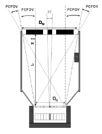
Figure 1: Scheme (not in scale) of the IBIS imaging system: a coded mask of $11.2\times 11.2\times 16$ mm³ tungsten elements, an upper low-energy detector plane (red) of 128$\times$128 CdTe crystals ($4\times 4\times 2$ mm³, pitch pixel-to-pixel = 4.6 mm), a high energy bottom detector plane (green) of 64$\times$64 CsI bars ($8.4\times 8.4\times 30$ mm³, pitch pixel-to-pixel = 9.2 mm), an active BGO veto system (blue) composed of 19 crystals viewed by photomultipliers, a passive shield made by a tube and a Hopper shield (grey), a calibration unit attached to the tube. The Fully Coded (= ${\rm arctan}[(D_{\rm M}-D_{\rm D})/L]$), and the Partially Coded, (= ${\rm arctan}[(D_{\rm M}+D_{\rm D})/L]$), Field of Views are indicated along with the telescope angular resolution (FWHM) $\Theta={\rm arctan}(H/L)$, where $D_{\rm D}$ and $D_{\rm M}$ are the detector and mask dimensions, $H$ is the width of the mask elements and $L$ the distance mask-detector ($\approx$ 3200 mm for ISGRI).

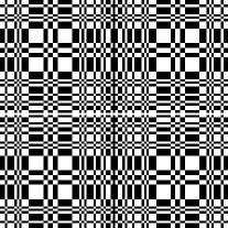
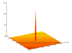
Figure 2: The IBIS mask pattern of 95$\times$95 elements (left) is formed by a replicated 53$\times$53 MURA basic pattern, whose cyclic autocorrelation (right) is a $\delta$ function.

The IBIS coded mask imaging system (Fig. 1) includes a replicated Modified URA (MURA)(Gottesman $\&$ Fenimore 1989) mask of tungsten elements (Fig. 2) and 2 pixellated gamma-ray detector planes, both approximately of the same size of the mask basic pattern: ISGRI, the low energy band (15 keV - 1 MeV) camera (Lebrun et al. 2003) and PICsIT, sensitive to photons between 175 keV and 10 MeV, disposed about 10 cm below ISGRI (Di Cocco et al. 2003). The physical characteristics of the IBIS telescope define a FCFOV of 8^∘ $\times$ 8^∘ and a total FOV (FCFOV+PCFOV) of 19^∘ $\times$ 19^∘ at half sensitivity and of 29^∘ $\times$ 29^∘ at zero sensitivity. The nominal angular resolution (FWHM) is of 12^′. ISGRI images are sampled in 5^′ pixels while PICsIT images in 10^′ pixels. The MURAs are nearly-optimum masks and a correlation inverse is obtained by setting $G=2M-1$ (i.e. $G=+1$ for $M=1$, $G=-1$ for $M=0$) apart from the central element which is set to 0. Simple correlation between such array and the detector plane array provides a sky image of the FCFOV where point sources appear as spikes of approximately the size (FWHM) of 1 projected mask element (12^′) with flat sidelobes (Fig. 2). The detailed shape of the System Point Spread Sunction (SPSF), the final response of the imaging system including the decoding process to the a point source, actually depends also on the instrument features (pixel size, detector deadzones, mask thickness, etc.) and on the decoding process (Gros et al. 2003). For this simple reconstruction (sum of transparent elements and subtraction of opaque ones) and assuming Poissonian noise, the variance in each reconstructed sky pixel of the FCFOV is constant and simply given by $V=G^{2}\star D=\sum_{kl}D_{kl}$, i.e. the total counts recorded by the detector. Therefore the source signal to noise is simply

$$S/N={C_{\rm S}\over{\sqrt{C_{\rm S}+C_{\rm B}}}}={{\rm Reconstructed\leavevmode\nobreak\ Source\leavevmode\nobreak\ Counts}\over\sqrt{\leavevmode\nobreak\ \rm Total\leavevmode\nobreak\ Counts}}$$

Sources outside the FCFOV but within the PCFOV still project part of the mask on the detector and their contribution can (and must) be reconstructed by properly extending the analysis in this region of the sky. In the PCFOV the SPSF does have secondary lobes (Fig. 3), the sensitivity decreases and the relative variance increases towards the edge of the field. In this part of the field also FCFOV sources will produce side lobes (see Sect. 2).

2 Sky image deconvolution

The discrete deconvolution in FCFOV can be extended to the total (FC+PC) FOV by performing the correlation of the detector array $D$ in a non cyclic form with the $G$ array extended and padded with 0 elements outside the mask. Since the number of correlated (transparent and opaque) elements in the PCFOV is not constant as in the FCFOV, the sums and subtractions for each sky position must be balanced and renormalized. This can be written by

$$S_{ij}={\sum_{kl}G^{+}_{i+k,j+l}W_{kl}D_{kl}\over\sum_{kl}G^{+}_{i+k,j+l}W_{kl}}-{\sum_{kl}G^{-}_{i+k,j+l}W_{kl}D_{kl}\over\sum_{kl}G^{-}_{i+k,j+l}W_{kl}}$$

where the decoding arrays are obtained from the G array by setting $G^{+}=G$ for $G>0$, $G^{+}=0$ for $G\leq 0$ and $G^{-}=-G$ for $G<0$, $G^{-}=0$ for $G\geq 0$, and then are enlarged and padded with 0’s outside the mask region. The sum is performed over all detector elements $k,l$ and $i,j$ run over all sky pixels (both of FC and PCFOV). In the FCFOV we obtain the same result of the standard FCFOV correlation. To consider effects such as satellite drift corrections (see Goldwurm 1995), dead areas, noisy pixels or other instrumental effects which require different weighing of pixels values, a specific array $W$ is used. For example $W$ is set to 0 for noisy pixels or detector dead areas and corresponding detector pixels are not included in the computation. The variance, which is not constant outside the FCFOV, is computed accordingly by

$$V_{ij}={\sum_{kl}(G^{+}_{i+k,j+l}W_{kl})^{2}D_{kl}\over(\sum_{kl}G^{+}_{i+k,j+l}W_{kl})^{2}}+{\sum_{kl}(G^{-}_{i+k,j+l}W_{kl})^{2}D_{kl}\over(\sum_{kl}G^{-}_{i+k,j+l}W_{kl})^{2}}$$

since the cross-terms $G^{+}$ and $G^{-}$ vanish. In the FCFOV the variance is approximately constant and equal to the total number of counts on the detector. The values computed by these formula are then renormalized to obtain the images of reconstructed counts per second from the whole detector for an on-axis source. Since mask elements are larger than detector pixels, the decoding arrays are derived as above after $G$ has been sampled in detector pixels by projection and redistribution of its values on a pixel grid. For non integer sampling of elements in pixels (the IBIS case) $G$ will assume continuous values from -1 to 1. Different options can be adopted for the fine sampling of the decoding array (Fenimore $\&$ Cannon 1981, Goldwurm 1995), the one we follow optimizes the point source signal to noise (while slightly spreading the SPSF peak). The SPSF, for an on-axis source and the IBIS/ISGRI configuration, obtained with the described deconvolution is shown in Fig. 3. Note the central peak and the flat level in the FCFOV, and the secondary lobes with the 8 main ghosts of the source peak at distances multiple of the mask basic pattern in the PCFOV. This procedure can be carried out with a fast algorithm by reducing previous formulae to a set of correlations computed by means of FFTs.

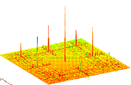
Figure 3: The System Point Spread Function over the complete FOV for the IBIS/ISGRI telescope.

3 Non-uniformity and background correction

In most cases and in particular at high energies the background is not spatially uniform. Further modulation is introduced on the background and source terms by the intrinsic detector non-uniformity. The modulation is magnified by the decoding process (the term $G\star B$ in Sect. 1) and strong systematic noise is generated in the deconvolved images (Laudet $\&$ Roques 1988). The resulting systematic image structures have spatial frequencies similar to those of the modulation on the detector plane. For the IBIS detector, intrinsic non-uniformity is generated by variations in efficiency of single detectors or associated electronics. Anticoincidence effects and scattering may also induce features at small spatial scales, of the order of the mask element size (Bird et al. 2003). The modulation induced by the external background is normally a large scale structure dominated by the differences in efficiency of the veto system and of multiple event tagging. The background intensity may be variable on timescales from hours/days (activation in radiation belts, solar flares) to weeks/months (orbit circularization, solar cycle modulation) (Terrier et al. 2003).

For the PICsIT layer, two more effects should be taken into account: the modulation at the border of the detector semimodules (Di Cocco et al. 2003) caused by the onboard multiple reconstruction system, and the cosmic-rays induced events. The former is due to the fact that multiple events are reconstructed by analysing events per semimodule. When a multiple event is detected by two semimodules, it is considered as two single events. Since this occurs at the borders of the semimodules, there is an excess of single events in these zones, and a corresponding deficit of multiple counts in the same pixels. Obviously this effect becomes important as the energy increases. In Fig. 5 it is shown an example of a single event shadowgram not yet corrected, where the border effects are clearly visible, and after the correction for background and non-uniformities (Natalucci et al. 2003). The second effect is due to spurious events caused by cosmic-rays interaction with CsI crystals (Segreto et al. 2003). This is relevant only at low energies ($<$ 250 keV) and results in a loss of sensitivity of about a factor of 4. It is possible to remove these fake events only if PICsIT is in photon-by-photon mode, while on the histograms it is possible to apply only an a-posteriori correction, by rescaling those pixels that, after the background subtraction, appear to be still noisy.

If the shape of the background does not vary rapidly, regular observations of source empty fields can provide measures of the background spatial distribution which can be used to flat-field the detector images prior to the decoding (contribution of weak sources is smoothed out by summing images corresponding to different pointing aspects) (Bouchet et al. 2001). If $U$ is the detector non-uniformity and $B$ the background structure, then the recorded detector image during an observation is $D=(S\ast M)U+B$ and a basic correction can be performed by $(D-bB_{EF})/U_{C}$, where $B_{\rm EF}$ is obtained from the empty field observations, $U_{\rm C}$ is an estimate of the detector non-uniformity from ground calibrations or Monte Carlo modelling and b is a normalization factor. If $U_{C}$ is a good estimate of $U$ and $B_{\rm EF}$ is close to $B$ we obtain the needed correction. The normalization $b$ is estimated either using the relative exposure times or the total number of counts in the images.

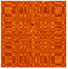
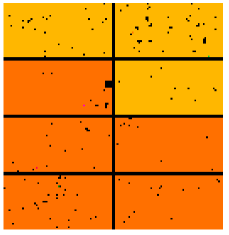
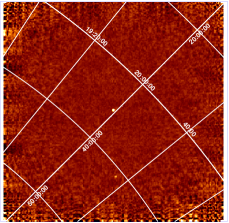
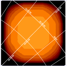
Figure 4: Results of reconstruction procedure applied to IBIS/ISGRI data of the Cygnus region: detector image after background correction (up, left), associated efficiency image (up, right), decoded and cleaned sky image in the whole FOV (FC+PC) (down, left), associated variance (down, right). The algorithm detected, and identified 2 sources: Cyg X-1 at the center of the FOV and Cyg X-3 in the PCFOV.

4 The IBIS scientific data analysis

The specific procedure for the IBIS data analysis starts from the data files obtained with the Integral Science Data Center (ISDC) (Courvoisier et al. 2003) preprocessing and performs a number of analysis steps which are hereafter described for the IBIS standard and photon-photon modes and the ISGRI and PICsIT data only.

The ISDC preprocessing decodes the telemetry packets, prepares the scientific and housekeping (HK) data with the proper satellite onboard times. This analysis task also computes the good time intervals by checking the satellite attitude, the telemetry gaps and the instrument modes and by monitoring the technological parameters. For the IBIS standard mode (Ubertini et al. 2003, Di Cocco et al. 2003) the following data sets are provided, for each elementary observation interval (science window) which corresponds to a constant pointing or slew satellite mode:
- ISGRI event list: position, arrival time, pulse-height channel, rise-time.
- PICsIT spectral-image histograms: 2 sets of $64\times 64$ pixel images in 256 energy channels, one for the integrated single events and the other for the integrated multiple events.
- PICsIT spectral timing histograms: count rates from the whole PICsIT camera integrated in a short time interval (0.97-500 ms, default: 2 ms) for up to 8 energy bands (default: 4 bands).
- Compton events list: ISGRI position, PICsIT position, ISGRI deposited energy, PICsIT deposited energy, ISGRI risetime, arrival time of events in coincidence between ISGRI and PICsIT.
For the IBIS photon-photon mode the same ISGRI and Compton data are provided while PICsIT histograms are replaced by
- PICsIT event list for single and double events: position, deposited energy, arrival time.
The first tasks performed by the IBIS specific software are the computation of the livetimes of the single pixels, of the deadtimes and of the deposited energies for all events. Detector images are then built and corrected. Sky images are reconstructed for each pointing and then combined to obtain mosaic of sky images of the whole observation. Source spectra are extracted by performing image binning and correction on small energy bands and then comparing resulting images to source models. All data products are written in files with the standard FITS and OGIP format in order to allow the use of standard high-level data analysis packages like FTOOLS, XSPEC and DS9.

4.1 Pixels livetimes, deadtimes and energy corrections

From the data of each single science window, prepared by the standard ISDC preprocessing, selected IBIS housekeeping (HK) data are first analyzed to prepare correction parameters for the scientific analysis. The HK tables reporting the initial status (on/off) of detector pixels, their low energy thresholds and their status evolution during the observations are decoded and the information organized to allow computation of livetime of each single pixel during the science window. The deadtime and its evolution is computed from the countrates reported in the HKs for the different IBIS datatypes, also including the time loss of random coincidences during veto rejection or calibration source tagging.

The ISGRI event pulse height channel and risetime information in the science data list are then used to reconstruct event deposited energy (in keV) by correcting the pulse height amplitude for the charge loss effect and for gains and offsets (Lebrun et al. 2003). The correction is performed using look-up tables (LUT) derived from ground and inflight calibrations (Terrier et al. 2003). PICsIT energies are reconstructed on board using gain and offset LUT before histograms are accumulated. A further correction on the PICsIT single events can be performed on ground by using pixel gain and offsets values refined according to temperature variations (Malaguti et al. 2003).

4.2 Image binning and uniformity-background correction

For each pointing science window the event list or the histograms are then binned in detector images for the specified energy bands and for a given risetime interval. The procedure computes an efficiency (or exposure) map combining informations from good time intervals, telemetry or data gaps, deadtimes, livetime of each pixel, and low energy thresholds. The map gives an exposure of each pixels considering all these effects and relative to an effective exposure time of the pointing.

ISGRI images are then enlarged to 130 $\times$ 134 pixels and PICsIT images to 65 $\times$ 67 pixels to include the deadzones between the modules. Residual noisy pixels, i.e. pixels with large values ($>5-10\leavevmode\nobreak\ \sigma$) above the average are then identified and efficiencies of noisy and deadzone pixels are set to 0. The detector image pixels are divided by the non-zero-values of the efficiencies to renormalize their values. For efficiencies equal to 0 the weighting array $W$ is set to 0 and the pixels are not included in the image or spectral reconstructions. The correction for detector and background non-uniformity is then applied using the background images derived from empty field observations and the detector uniformity maps (Terrier et al. 2003, Natalucci et al 2003). For the spectral extraction however the correction is not perfomed at this level, background and non-uniformity are accounted for directly in the fitting procedure.

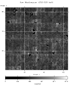
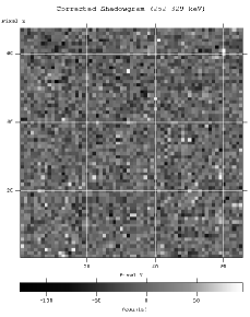
Figure 5: Results of the background correction on a PICsIT single event shadowgram (252-329 keV) of the Crab region. The raw image (left) shows presence of dead pixels and count excess on the module borders, not visible in the background corrected image (right).

4.3 Iterative sky image reconstruction and cleaning

From the corrected detector images the analysis procedure decodes the sky images using the algorithm described in Sect. 2 and iteratively searches for significant peaks in the image. The signal to noise levels (S/N) of detection can be set by the users, and the search can be preferencially performed or even totally restricted to the sources included in an input catalogue. The search procedure is a delicate process due to the presence of the 8 ghosts (per source) and is sensitive to the choices of the S/N levels of search in particular if the background is not fully corrected. The first significant peak is detected and fitted with an analytical approximation of the SPSF to finely determine the position of the source and its flux (Gros et al. 2003). The model of the shadowgram projected by the source at the derived position is computed, decoded, normalized to the observed excess and subtracted from the image. Such a source response model must take into account the mask element thickness, the effects at the mask border, the different opacity of the mask support and of the passive shield, and the transparent zones in or between these elements. However the model includes only the geometrical absorption effects. Proper account of scattering and energy redistribution is included in the energy response. The same routine which computes the model of source shadowgram on the detector is used in the spectral extraction. The source parameters (position, flux, and signal to noise) are stored in an output file and the procedure uses the source catalogue to identify the source. A second excess is then searched and cleaned and the procedure continues till all sources or excesses are identified and cleaned. The image of the main peak of each source is finally restored in the sky image while the secondary lobes are excluded. Units of intensity images are in reconstructed counts per second for an on-axis source, and a variance image is computed in the proper units.

4.4 Image mosaic and final image analysis

The reconstructed and cleaned sky images of each pointing science window are then rotated, projected over a reference image and summed after a properly weighting with their variance and exposure time. There are two ways to implement the rotation of an image. Either the pixel value is redistributed around the reference pixels on which is projected or its value is entirely attributed to the pixel whose center is closer to the projected center of the input pixel. In the first case the source is slightly smoothed and enlarged but the source centroid is well reconstructed, while in the second case discrete effects can produce a bias in the source centroid but the intensity will be better reconstructed and the source less spread.

After the mosaic step is completed the routine restart the search and analysis of point sources in the mosaicked sky image, again using a catalogue for the identification. Results of fluxes and positions are reported in output. Since the point source location error is inversely proportional to the source signal to noise (Gros et al. 2003), location of weak sources is better carried out on mosaicked images. Note that the search for significant excesses (both for single pointing and for the mosaic) must be performed taking into account that these are correlation images and considering the number of independent trials that are made by testing all pixels of the reconstructed sky image. The critical level at which an unknown excess is significant must be increased from the standard 3 $\sigma$ value to typically 5 - 6 $\sigma$ (see e.g. Caroli et al. 1987). In the case of residual (background) systematic modulation, the detection level must be further increased (for example by a factor given by the ratio of measured to computed image standard deviation).

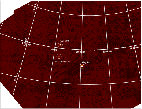
Figure 6: Sky image mosaic of the Cygnus region in the 15-40 keV band composed with IBIS/ISGRI data from 130 pointings for a total exposure of 145 ks. Three sources are detected at high significance level: Cyg X-1, Cyg X-3 and EXO 2030+375.

4.5 Source spectra and light curve extractions

Once the positions of the active sources of the field are known, their fluxes and count spectra are extracted for each pointing science window in predefined energy bins. Detector images and their efficiencies are built for these energy bins, enlarged and then searched for residual noisy pixels. For each source and each energy band a shadowgram model is then computed using the detailed modelling algorithm described above. If $P_{kl}^{n}(\Delta E_{h})$ is the model for the source n and the energy bin $\Delta E_{h}$, the total sky plus background model $T$ at the pixel $k,l$ is defined as

$$T_{kl}^{m}(\Delta E_{h})=\sum_{n=1}^{m}f_{n}^{h}P_{kl}^{n}(\Delta E_{h})E_{kl}^{h}U_{C}^{h}+b^{h}B_{kl}(\Delta E_{h})E_{kl}^{h}$$

where the sum is extended to all ”active” sources of the region and where the background image $B$ is derived from the empty field data, the $U_{\rm C}$ is the estimated detector non-uniformity and $E$ is the efficiency image. This model is fitted to the enlarged and noisy-pixel-corrected detector images $D_{k,l}$ by using the maximum likelihood technique with Poissonian distribution. The optimization gives the multiplicative factors $f_{n}^{h}$ and $b^{h}$ for each energy band which (after proper normalizations and division by the exposure time), provide the source and background count rate spectra. It is important to perform the simultanous fit for the models of all the active sources of the field to avoid contamination by other sources of the interested spectrum. Spectra of the same source collected in different pointing science windows can then be summed to obtain an average spectrum during an observation. The spectra are compared to physical spectral models convolved with the energy response function of the instrument (Laurent et al. 2003) in order to evaluate source physical parameters. Finally, a similar procedure, where the images are binned in large energy bands and small time intervals, provides source light curves on time bins shorter than science windows for the predefined active sources in the field of view. For PICsIT operating in standard mode, light curves of the count rates registered by the whole detector can be generated directly from the spectral timing data and used to search for characteristic variability signatures like pulsations or bursts.

5 Final remarks

The software has been tested using inflight data in several conditions and the performance is satisfactory considering the early phase of the mission. Background corrections have been already implemented for the analysis of PICsIT data while not yet fully used for the ISGRI analysis (but see Terrier et al. 2003). Fig. 5 shows the correction operated on the Crab nebula PICsIT images as described in Sect. 3. In Fig. 6 the resulting sky image mosaic obtained from the IBIS scientific pipeline applied to about 130 elementary pointings on Cygnus X-1, illustrate the quality of the scientific analysis presently available. Images are well reconstructed and cleaned and sources well detected and finely positioned, with typical absolute error radii (90$\%$ confidence level) of less 1^′ for strong source (S/N $>$ 30-40) and less than 3^′ for moderate or weak ones (S/N $\approx$ 10-40) (Gros et al. 2003). Fig. 7 shows a reconstructed PICsIT image of the Crab, a very bright constant and pointlike source for IBIS, often used as calibration source for high energy instruments. Fig. 8 reports a reconstructed Crab count spectrum obtained with the described scientific analysis procedures from the ISGRI data of an observation pointed on the source and performed in staring mode (constant attitude asset during the observation, see Winkler et al. 2003). The spectrum is compared to a model of a simple power law using the instrument energy response files. The best fit in the range 20-700 keV is found for a slope of 2.05 which is compatible with the high energy spectrum of the Crab. To have acceptable $\chi^{2}$, systematic errors of about 10$\%$ have to be included.

These examples give an idea of the performance of the analysis s/w and of the calibration and response files presently available. The procedures described here have been integrated in the ISDC analysis system and constitute the core of the IBIS data analysis software of the Quick Look and Standard Analysis run at the ISDC and of the INTEGRAL Data Analysis System package. The IBIS analysis software and associate calibration files are constantly improved and integrated in the following versions of the ISDC system. The present set has already been used to derive a number of interesting results from the IBIS data of the high energy sources observed with INTEGRAL (see this volume).

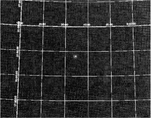
Figure 7: IBIS/PICsIT reconstructed image of the Crab in the energy band 252-329 keV obtained from the IBIS scientific pipeline applied to 55 science windows for a total of 132 ks of exposure.

Figure 8: IBIS/ISGRI reconstructed count spectrum of the Crab from data of a 90 ks exposure pointed observation. The best fit model of a power law and ratios are also shown. The ratios show presence of 10$\%$ systematic erros in particular in the 20-100 keV range.

References

- Bird et al. (2003) Bird, A.J., Barlow, E.J., Bazzano, A., et al., 2003, A&A, this issue
- Bouchet et al. (2001) Bouchet, L., Roques, J.-P., Ballet, J., Goldwurm, A., Paul, J., 2001, ApJ, 548, 990
- Caroli et al. (1987) Caroli, E., Stephen, J.B., Di Cocco, G., Natalucci, L., Spizzichino, A., 1987, Space Sci. Rev., 45, 349
- Courvoisier et al. (2003) Courvoisier, T.J.-L., Walter, R., Beckmann, V., et al., 2003, A&A, this issue
- Di Cocco et al. (2003) Di Cocco, G., Caroli, E., Celesti, E., et al. 2003, A&A, this issue
- Fenimore & Cannon (1978) Fenimore, E.E. & Cannon T.M., 1978, Appl. Opt., 17(3), 337
- Fenimore & Cannon (1981) Fenimore, E.E. & Cannon T.M., 1981, Appl. Opt., 20(10), 1858
- Goldwurm (1995) Goldwurm, A., 1995, Exper. Astron., 6, 9
- Goldwurm et al. (2001) Goldwurm, A., Goldoni, P., Gros, A., et al., 2001, In: Proc. of the 4th INTEGRAL Workshop, A. Gimenez, V. Reglero and C. Winkler. (eds). ESA-SP 459, p. 497
- Gottesman & Fenimore (1989) Gottesman, S.R. & Fenimore, E.E., 1989, Appl. Opt., 28, 4344
- Gros et al. (2003) Gros, A., Goldwurm, A., Cadolle-Bel, M., et al., 2003, A&A, this issue
- Laudet & Roques (1988) Laudet, P., & Roques, J.P., 1988, N.I.M.P.R., A267, 212
- Laurent et al. (2003) Laurent, P., Limousin, O., Cadolle-Bel, M., et al. 2003, A&A, this issue
- Lebrun et al. (2003) Lebrun, F., Leray, J.-P., Lavocat, P., et al., 2003, A&A, this issue
- Malaguti et al. (2003) Malaguti, G., Bazzano, A., Bird, A.J., et al., 2003, A&A, this issue
- Natalucci et al. (2003) Natalucci, L., Bird, A.J., Bazzano, A., et al. 2003, A&A, this issue
- Paul et al. (1991) Paul, J., Ballet, J., Cantin, M., et al. 1991, AdSpR, 11(8), 289
- Segreto et al. (2003) Segreto, A., Labanti, C., Bazzano, A., et al., 2003, A&A, this issue
- Skinner (1995) Skinner, G.K., 1995, Exper. Astron., 6, 2
- Terrier et al. (2003) Terrier, R., Lebrun, F., Bazzano, A., et al., 2003, A&A, this issue
- Ubertini et al. (2003) Ubertini, P., Lebrun, F., Di Cocco, et al., 2003, A&A, this issue
- Winkler et al. (2003) Winkler, C., Courvoisier, T.J.-L., Di Cocco, G., et al., 2003, A&A, this issue