Monte Carlo radiative transfer
in molecular cloud cores

We present the results of a three-dimensional Monte Carlo radiative transfer code for starless molecular cloud cores heated by an external isotropic or non-isotropic interstellar radiation field. The code computes the dust temperature distribution inside model clouds with specified but arbitrary density profiles. In particular we examine in detail spherical (Bonnor-Ebert) clouds, axisymmetric and non-axisymmetric toroids, and clouds heated by an external stellar source in addition to the general interstellar field. For these configurations, the code also computes maps of the emergent intensity at different wavelengths and arbitrary viewing angle, that can be compared directly with continuum maps of prestellar cores. In the approximation where the dust temperature is independent of interactions with the gas and where the gas is heated both by collisions with dust grains and ionization by cosmic rays, the temperature distribution of the gas is also calculated. For cloud models with parameters typical of dense cores, the results show that the dust temperature decreases monotonically from a maximum value near the cloud’s edge (14–15 K) to a minimum value at the cloud’s center (6–7 K). Conversely, the gas temperature varies in a similar range, but, due to efficient dust-gas coupling in the inner regions and inefficient cosmic-ray heating in the outer regions, the gradient is non-monotonic and the gas temperature reaches a maximum value at intermediate radii. The emission computed for these models (at 350 $\mu$m and 1.3 mm) shows that deviations from spherical symmetry in the density and/or temperature distributions are generally reduced in the simulated intensity maps (even without beam convolution), especially at the longer wavelengths. adiative transfer; ISM: clouds, dust, extinction

1 Introduction

Understanding the structure of pre–protostellar cores is an essential step towards an understanding of protostellar evolution. The density distribution immediately prior to the onset of gravitational collapse defines the initial conditions for collapse and hence one has a strong motivation to attempt to derive this density distribution from the observations. Since these objects are most commonly observed by means of their millimeter dust emission, one has a strong interest in understanding the temperature distribution of the dust in the pre–protostellar core and its influence on the emergent intensity distribution at millimeter-submillimeter wavelengths. In this article, we present a radiative transport code which has the interpretation of mm-submm maps of pre–protostellar cores as its main goal.

The approach which we have adopted is influenced by the fact that, as a rule, the density structure of these objects shows evidence for large deviations from spherical symmetry. More precisely, the maps of the millimeter dust emission show clear departures from circular symmetry (see e.g. André et al. 2000; Caselli et al. 2002a,b; Tafalla et al. 2002). In some cases there is also evidence for polarization and hence for a magnetic field (Ward-Thompson et al. 2000). It seems likely to us that such behavior is caused by magnetic fields of energy densities sufficiently large to influence the core structure (see also Shu et al. 1987) and cause flattening along field lines (Basu 2000, Jones & Basu 2002). We can attempt to infer the density distribution on the basis of mm-submm continuum maps if we can derive the temperature distribution in regions where departures from spherical symmetry are important. A first attempt in this direction was made by Zucconi et al. (2001, hereafter ZWG, see also Evans et al. 2001 for the spherically symmetric case) but these authors neglected heating of dust grains due to re-absorption of photons emitted by the cloud itself. Here we present a Monte–Carlo code without this limitation but which is capable of handling a variety of geometries. We expect that this type of analysis will be especially useful as a tool for the interpretation of the high class data we expect to come from future instruments like ALMA and HERSCHEL.

Some high quality data are already available and are consistent with a picture in which the dust temperature of pre-protostellar cores decreases towards the center (Ward-Thompson et al. 2002, Bianchi et al. 2003). ISO observations in the mid-IR (Bacmann et al. 2000) and in the far-IR (Ward-Thompson et al. 2002) suggest dust temperature gradients consistent with heating from the external interstellar radiation field (ISRF). The available models predict a factor of $\sim 2$ increase in temperature from center to edge (ZWG, Evans et al. 2001, André et al. 2003), with the gradient dependent on the cloud structure. The predicted emission of several cores is in reasonable accord with the data, and implies that the assumed equilibrium configurations are either unstable or maintained by a magnetic field.

Additional observational constraints on the thermal structure of prestellar cores are given by spatially resolved measurements of the gas temperature from NH₃ observations. Low-mass cores show fairly uniform gas temperature (e.g. Tafalla et al. 2002 for L1517B and L1498), whereas massive quiescent cores in Orion show significant temperature drops from edge to center (Li et al. 2003). Thus another check on our understanding of core structure is possible if radiative transfer models are also able to predict the gas temperature distribution resulting from the balance of the relevant heating and cooling mechanisms. We therefore have also developed the capability to predict gas temperature distributions for our model cores.

While techniques have been developed for the study of radiative transfer in cold cores in one dimension (e.g. Leung 1976, Rowan-Robinson 1980, Ivezic et al. 1997), their extension to three-dimensional geometries is not straightforward. A Monte Carlo technique has the advantage that it deals easily with any general geometry, independently of the density distribution and the anisotropy of the incident radiation field. The increasingly faster workstations available render this technique very useful, and fully 3-D Monte Carlo radiative transfer codes have been developed recently (e.g. Wolf et al. 1999, Niccolini et al. 2003). However, in these latter studies the radiative sources are internal, and this is a computationally distinct problem from a core heated from the outside for two main reasons. First, as we are interested in cold cores, it is reasonable to expect that they will be optically thin to their own emission, and therefore, for methods that use iteration, the temperature distribution quickly relaxes to the final value; alternatively, for methods that follow individual packets until they exit the domain, each individual packet will interact with the dust often only once. Second, as packets are launched from the outside, a wide range of spatial scales demands a prohibitively large photon statistics, as the probability of a packet being launched in the direction of the innermost cells becomes increasingly small.

In general, our paper confirms and supports the results recently obtained for embedded prestellar cores by Stamatellos & Whitworth (2003) with an independent but similar Monte Carlo radiative transfer code. While Stamatellos & Whitworth (2003) focus on the important effect of the ambient medium in which (spherical) cores are embedded, our paper mostly emphasizes the consequences of deviations from spherical symmetry in the density distribution and anisotropies of the ISRF. The two papers represent therefore complementary attempts to model radiative transfer in molecular cloud cores in less idealized situations than those considered so far.

The structure of this paper is as follows. In Sect. 2, we set the general problem of radiative transfer in a dusty cloud. In Sect. 3, we describe the Monte Carlo method we have used. In Sect. 4, we present our choice of opacities and interstellar radiation field and briefly discuss their effect in the results. In esections 5 and 6 we present our results for two- and three-dimensional models, respectively. Finally, in Sect. 7 we summarize our conclusions.

2 Radiative transfer in a dusty cloud

In local thermodynamic equilibrium and ignoring the effects of scattering of radiation by dust grains, the radiation field in a dusty cloud satisfies the equation of transfer

$${\hat{\bf n}}\cdot\nabla I_{\nu}({\bf r},{\hat{\bf n}})=\rho({\bf r})\kappa_{\nu}({\bf r})\{B_{\nu}[T_{\rm d}({\bf r})]-I_{\nu}({\bf r},{\hat{\bf n}})\},$$ (1)

where $I_{\nu}({\bf r},{\hat{\bf n}})$ is the specific intensity of radiation (in Jy ster^-1) at position ${\bf r}$ in the direction ${\hat{\bf n}}$ at frequency $\nu$, $\rho$ is the total (gas plus dust) density, $\kappa_{\nu}$ the total absorption opacity, $T_{\rm d}$ is the dust temperature, and $B_{\nu}$ is the Planck function,

$$B_{\nu}(T_{\rm d})=\frac{2h\nu^{3}}{c^{2}}\left[\exp\left(\frac{h\nu}{kT_{\rm d}}\right)-1\right]^{-1}.$$ (2)

The dust temperature distribution $T_{\rm d}({\bf r})$ is obtained by solving the equation of balance of emitted and absorbed radiation,

$$\int^{\infty}_{0}\kappa_{\nu}B_{\nu}[T_{\rm d}({\bf r})]\;d\nu=\int^{\infty}_{0}\kappa_{\nu}J_{\nu}({\bf r})\;d\nu,$$ (3)

where

$$J_{\nu}({\bf r})=\frac{1}{4\pi}\oint I_{\nu}({\bf r},{\hat{\bf n}})\;d\Omega$$ (4)

is the mean intensity of radiation (in Jy).

ZWG made the symplifying assumption that the dust grains are only heated by the incident interstellar radiation field $J_{\nu}^{\rm ISRF}$ (assumed isotropic), neglecting re-emission of radiation absorbed by the grains themselves. That is to say, they assumed that the cloud is optically thin to its own radiation. Under this hypothesis, the equation of radiative transfer has the solution

$$J_{\nu}({\bf r})=\frac{J_{\nu}^{\rm ISRF}}{4\pi}\oint\exp[-\tau_{\nu}({\bf r},{\hat{\bf n}})]\;d\Omega,$$ (5)

where

$$\tau_{\nu}({\bf r},{\hat{\bf n}})=\int^{{\hat{\bf n}}R}_{r}\rho({\hat{\bf r}}r^{\prime})\kappa_{\nu}({\hat{\bf r}}r^{\prime})\;dr^{\prime},$$ (6)

is the optical depth from a point ${\bf r}$ inside the cloud to a point ${\hat{\bf n}}R$ on the cloud boundary, in the direction ${\hat{\bf n}}$. The calculation of the radiation field inside the cloud is thus reduced to a large number of integrations along different directions (rays) defined at each grid point. This simplification allowed ZWG to model axisymmetric non-spherical density distributions, but has the disadvantage of slightly underestimating the dust temperature, particularly at the cold center of the cloud.

Our general approach is the following. First, for a given ISRF we compute the radiation field at any point inside the cloud core and solve the equation of balance of radiation emitted and absorbed by dust grains to obtain the dust temperature distribution $T_{\rm d}({\bf r})$. Second, we compute the flux emitted in a given view direction at different wavelengths and we compare the results with observed spectral energy distributions and monochromatic maps for specific objects.

In several cases we have also considered the effect of a spherical envelope surrounding the cloud core on the resulting temperature distribution. The rationale for this is that these objects are always embedded in a photon–dominated region (PDR) which transforms the incident optical–UV field into mid and far IR radiation. Often in practice, this is radiation from transiently heated particles, either small grains or polycyclic aromatic hydrocarbons, emitting in the 3–30 $\mu$m range. Since we wish to focus on the temperature structure of the high density core interior, we have decided to assume that the radiation field incident on embedded cores is cut off in the optical-UV wavelength range and that the radiation absorbed in the PDR is reradiated in the infrared. We thus incorporate the photons reradiated by the PDR in the external field. The error involved here can be estimated by varying the form of the ISRF and appears to be small (though see the discussion of André et al. 2003). Our focus here is on the effects of the core geometry upon temperature structure and we place minor emphasis on the spectral energy distribution of the incident field.

We stress that our approach is general: the density distribution, the optical properties of the dust grains, the intensity and spectral energy of the radiation source(s) are input parameters that can be freely specified and can be adapted to model various astrophysical situations.

3 The Monte Carlo method

In the Monte Carlo technique, the computational domain is divided in a large number of cells of mass $m_{i}$ that absorb and emit radiation. The energy that enters the computational domain is divided in $N_{\gamma}$ monochromatic packets of equal energy, that are launched stochastically from the boundary and followed until they exit the cloud. These packets may be absorbed by the dust particles, resulting in a temperature increase of the cells where they are absorbed, and are immediately reemitted to enforce radiative equilibrium. If the cell $i$ absorbs $N_{i}$ packets, the energy absorbed by the cell per unit time is

$$\frac{dE_{i}^{\rm abs}}{dt}=\left(\frac{N_{i}}{N_{\gamma}}\right)L^{\rm ISRF},$$ (7)

where $L^{\rm ISRF}$ is the luminosity of the ISRF at the cloud’s surface, obtained integrating the mean intensity of the (anisotropic) ISRF over the cloud’s surface and over frequency,

$$L^{\rm ISRF}=\int_{0}^{\infty}d\nu\oint d\Omega\oint J^{\rm ISRF}_{\nu}({\hat{\bf n}}){\hat{\bf n}}\cdot d{\bf S}.$$ (8)

Assuming LTE conditions, the energy emitted by the $i$-th cell per unit time is

$$\frac{dE_{i}^{\rm em}}{dt}=4\pi m_{i}\int_{0}^{\infty}\kappa_{\nu}B_{\nu}(T_{{\rm d},i})\,d\nu$$ (9)

where $T_{{\rm d},i}$ is the dust temperature of the $i$-th cell, obtained by equating the absorbed and emitted energies per unit time,

$$\int^{\infty}_{0}\kappa_{\nu}B_{\nu}(T_{{\rm d},i})\;d\nu=\left(\frac{N_{i}}{N_{\gamma}}\right)\frac{L^{\rm ISRF}}{4\pi m_{i}}.$$ (10)

The integral on the left-hand side of this equation can be tabulated for a grid of values of the dust temperature and opacity. The solution of Eq. (10) can then be easily obtained by iteration and interpolation. In the limit to the continuum, $N_{\gamma}\rightarrow\infty$ and $m_{i}\rightarrow 0$, Eq. (10) is equivalent to Eq. (3), but differs from the approximation adopted in ZWG, Eq. (5), because in $N_{i}$ are included the packets that may have been absorbed more than once in the cloud, and subsequently re-emitted.

We handled re-radiation (and, therefore, energy conservation) using the method devised by Bjorkman & Wood (2001): once a packet is absorbed, it is immediately re-emitted (to conserve energy) at a new frequency determined by the local dust temperature. To achieve this, one starts by noting that if a cell has emissivity $\kappa_{\nu}B_{\nu}(T_{{\rm d},i}-\Delta T_{{\rm d},i})$ prior to absorbing a wave packet, then after packet absorption its temperature increases by an amount $\Delta T_{{\rm d},i}$, and the cell emissivity becomes $\kappa_{\nu}B_{\nu}(T_{{\rm d},i})$. Thus, the increment in the cell emissivity is

$$\Delta j_{\nu} = \kappa_{\nu}[B_{\nu}(T_{{\rm d},i})-B_{\nu}(T_{{\rm d},i}-\Delta T_{{\rm d},i})]$$ (11)

$$\simeq\kappa_{\nu}\left(\frac{dB_{\nu}}{dT_{\rm d}}\right)_{T=T_{{\rm d},i}}\Delta T_{{\rm d},i}.$$

A photon packet is immediately reemitted with a frequency obtained from a probability distribution having the same spectral shape as $\Delta j_{\nu}$,

$$\frac{dP_{i}}{d\nu}=\frac{\kappa_{\nu}}{K}\left(\frac{dB_{\nu}}{dT_{\rm d}}\right)_{T=T_{{\rm d},i}},$$ (12)

where $K=\int^{\infty}_{0}\kappa_{\nu}(dB_{\nu}/dT_{\rm d})\;d\nu$ is a normalization constant. The re-emitted photon packet is then followed until a new interaction occurs, and the procedure is repeated until the photon leaves the cloud. This method ensures energy conservation in a statistical sense. Due to the low temperature of the cores, energy is generally re-radiated at long wavelengths, to which the core has a low optical depth, and the overall effect of re-emission on the dust temperature is more significant in the core’s cold interior but is generally very small.

3.1 Tests of the code

We have tested our Monte Carlo code in different ways. Here we present the results of two complementary tests, one checking the accuracy of the packet propagation procedure and one checking the equality of emitted and absorbed energy.

To test the packet propagation procedure, we have computed dust temperatures profiles for spherically symmetric clouds, for which results can also be obtained with the ray integration method of ZWG. Specifically we have assumed the density profile of a Bonnor-Ebert (BE) sphere, an isothermal, pressure-bounded, equilibrium model, that reproduces the centrally flattened density distribution and the rapid density decrease at large radii observed in most cloud cores. Fig. 1 shows the dust temperature as function of radius for a BE with radius $R=0.1$ pc, central density $n({\rm H}_{2})=4.4\times 10^{6}$ cm^-3, and isothermal gas temperature $T_{\rm g}=12$ K (note that the gas temperature here is merely for the purpose of specifying the assumed density distribution). As shown in Fig. 1, the result obtained using the ray integration method (solid line), is identical to the Monte Carlo result using the same approximation of optically thin re-emission (dotted line). We also notice that when re-emission is taken into consideration (dashed line), there is only a small increase of the central temperature, even in this case, when the extinction through the core center is $A_{2.2\mu\rm{m}}\simeq 25$, and the central dust temperature is little more than 6 K.

To test energy conservation, we have computed the energy emitted per unit time by an arbitrary area element on the cloud’s surface by integrating $I_{\nu}$ (the solution of eq. 1) and $I_{\nu}^{\rm ISRF}$ over solid angles and frequencies, finding a very small discrepancy between the two values (less than 1 %). This test shows that for the given number and size of cells, the accuracy of Eq. (10) and (12), that contain approximations introduced by the discretization of the computational volume, is very good.

4 Dust opacities and the interstellar radiation field

4.1 The interstellar radiation field

Following ZWG and Evans et al. (2001), we adopt as a reference the ISRF given by Black (1994), which is an average for the solar neighbourhood. Scaling the intensity of the ISRF by a factor $G_{0}$ leads to a change in the dust temperature at all radii by a factor of ${G_{0}^{1/(4+\beta)}}$, where $\beta\simeq 2$ is the power law index for the long wavelength opacity. Actually the radiation incident on molecular cloud cores may differ not only in intensity but also in spectral shape, depending on the degree of embedding of the cores in the ambient cloud and on the possible vicinity to hot stars. It appears for example to be the case that many cores associated with the $\rho$ Oph star forming regions are subjected to an incident ISRF roughly an order of magnitude larger than the solar neighbourhood ISRF. An example of what can happen is given by a recent study by André et al. (2003) of a particular core, heated by a ISRF higher than the Black field by an order of magnitude in both the mid-IR and far-IR. This resulted in a higher central temperature and a sharper gradient at the edge than in our models for a similar density distribution. Thus observers attempting to infer density distributions from maps of the mm–submm dust emission must bear in mind the fact that both the radiation field and the geometry can play a role.

In this paper however, our objective is to study the effects of geometry rather than those of the spectral characteristics or intensity of the incident radiation field. Geometry in this context can mean the geometry of the density distribution or that of the radiation field. We thus also consider a case where we use our Monte Carlo model to consider an anisotropic incident ISRF as exists in many galactic reflection nebulae.

4.2 Dust opacities

We adopt the dust opacities tabulated by Ossenkopf & Henning (1994, hereafter OH) in the wavelength range 1 $\mu$m–1.3 mm. Recent work by Bianchi et al. (2003) and by Kramer et al. (2003) has shown that these theoretically derived opacities are consistent with the observed ratio of mm dust continuum intensity and near infrared extinction. It is also clear from the study by OH that one can expect the dust opacity to vary between the lower density outer layers of a core and the high density interior where most of the heavy element content of the core is in the form of ice of various sorts. We neglect such effects in this study mainly because, as shown below, the variation between different OH dust models is relatively mild.

We label the opacity according to the column number in Table 1 of OH: OH1, standard MRN distribution; OH4, MRN with thin ice mantles; OH5, MRN with thin ice mantles, after $10^{5}$ yr of coagulation at density $10^{6}$ cm^-3; OH8, MRN with thick ice mantles, after $10^{5}$ yr of coagulation at density $10^{6}$ cm^-3.

The OH opacities are tabulated for wavelengths between 1 $\mu$m and 1.3 mm. Within this range we have obtained values of the opacity at arbitrary wavelengths by four-point interpolation and above 1.3 mm, we have used a power law extrapolation based on the last two tabulated values. We neglect scattering completely as we are interested in the transport of infrared photons.

The effect of the various opacities on the temperature profile of a cloud is shown in Fig. 2, for the reference case of a BE sphere with central density $n({\rm H}_{2})=4.4\times 10^{6}$ cm^-3, radius 0.1 pc, gas temperature $T_{\rm g}=12$ K, embedded in a spherical envelope with total extinction $A^{\rm env}_{2.2\mu{\rm m}}=0.1$. In this particular example, the gas-to-dust ratio was varied for each opacity prescription in order to keep fixed the total extinction at 2.2 $\mu$m.

As Fig. 2 shows, temperature variations due to different choices of the opacity are generally small. The opacities OH1, OH4 and OH5 have a similar dependence on wavelength, and the resulting temperature difference is equivalent to scaling the intensity of the ISRF by about $10\%$. The OH8 opacity, having a slightly different dependence on wavelength, results in a the temperature profile slightly different from the other three cases. In all remaining models presented in this study we have used OH5.

5 Two-dimensional models

In this section we consider two particular situations that require a two-dimensional modeling of the radiative transfer. In the first example, the external radiation field is isotropic but the density distribution is not spherically symmetric. In the second example, the density profile is spherically symmetric but the incident radiation field is anisotropic, as the cloud is heated by an external stellar source. Both situations are easily handled by our Monte Carlo code.

5.1 Singular isothermal toroids

As a first application of our Monte Carlo code, we consider the radiative transfer in a singular isothermal toroid (Li & Shu 1996), a scale-free, axisymmetric equilibrium configuration of an isothermal cloud under the influence of sef-gravity, gas pressure and magnetic forces. These toroids are characterized by a single parameter, $H_{0}$, representing the fractional amount of support provided by the magnetic field. We choose the particular value $H_{0}=0.5$ to model a cloud with moderate axial ratio ($\sim 2.5$) intermediate between a spherical unmagnetized cloud and a magnetically dominated disklike configuration.

It should be noticed that, in all models presented, we are simply computing the dust temperature of pre-defined core density distributions, and therefore the resulting core is not the solution of the equilibrium equation if gas-dust coupling is assumed. Also, the practical definition of the boundary as an isobaric surface is only possible for spherical clouds, as in this case the isopycnic and isobaric surfaces necessarily coincide. In all other geometries, we take the boundary as the isopycnic surface corresponding to a specified value of the density.

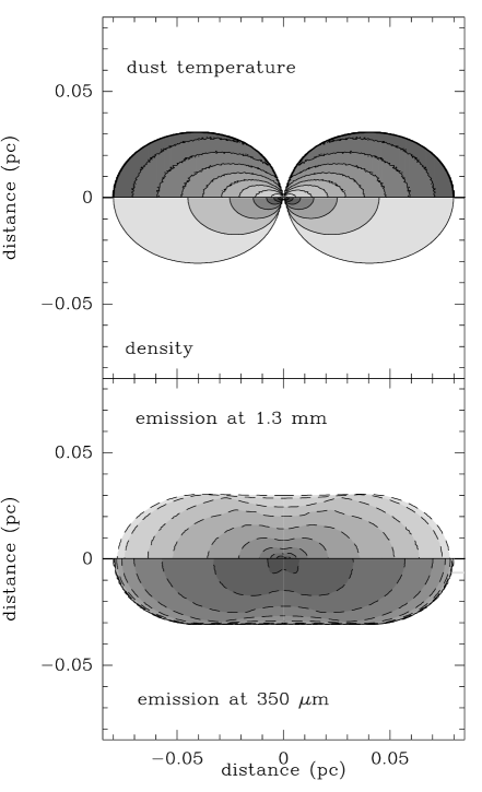
Figure 3: The top panel shows the dust temperature (top half) and density distribution (bottom half) of a singular isothermal toroid with $H_{0}=0.5$, seen edge-on. The density on the boundary is $n({\rm H}_{2})=10^{4}$ cm^-3 and the isopycnic curves are logarithmically spaced by 0.5. The density distribution is azimuthally symmetric and also symmetric with respect to the midplane. The maximum outer temperature is 15 K and the isothermal curves are spaced by 1 K. The bottom panel shows the emission at 1.3 mm (top half) and at 350 $\mu$m (bottom half). The isophotal curves are logarithmically spaced by 0.2 starting from the lower value $0.01\times I_{\nu}^{\rm max}$. With the adopted opacity law (OH5), the peak values are $I_{\nu}^{\rm max}=77$ MJy sr^-1 at 1.3 mm and 382 MJy sr^-1 at 350 $\mu$m (in this and in the following figures, the maps have not been convolved with an observing beam).

In Fig. 3 are shown both the density distribution of the toroid and the resulting temperature distribution. The boundary of the configuration is defined as the isopycnic surface with $n({\rm H}_{2})=10^{4}$ cm^-3. We choose this value of the density because it represents the threshold value that characterizes typical dense (“ammonia”) cores. For a density profile characterized by a $r^{-2}$ law, the visual extinction of the cloud material with density below this threshold value corresponds to about $A_{V}\simeq 2$–3. Notice that the temperature varies over the boundary surface by a factor of about two from the origin to the maximum radius, and this difference is due to an increase of grain exposure to the ISRF as the radius increases, an effect known also for disks of low aspect ratio (e.g. Spagna et al. 1991), and is particularly enhanced in a toroid. It is also evident from Fig. 3 that the temperature decreases outward both in the horizontal and vertical directions.

In Fig. 3, we also show synthetic (unconvolved with an observing beam) maps of the expected dust emission at 350 $\mu$m and 1.3 mm. In particular at 1.3 mm, the “observed contours” reflect fairly faithfully the projected column density and hence the density distribution. At 350 $\mu$m however, the intensity distribution is much more extended than at 1.3 mm. The half-power dimensions are $\sim 1.5^{\prime\prime}\times 3.7^{\prime\prime}$ at 1.3 mm (in angular size at a distance of 140 parsec) but $18^{\prime\prime}\times 25^{\prime\prime}$ at 350 $\mu$m. Thus the effect of heating from the exterior is mainly observable as an increase in size with frequency.

5.2 Anisotropic Radiation Field

While the above discussion concerns cores of non-spherical geometry subject to an isotropic incident radiation field, it should be noted that one expects often to find cases where the incident radiation field is anisotropic. Most obviously, this is the case in galactic reflection nebulae where the radiation field from single early type stars may be dominant. We therefore here (in a slight parenthesis to the discussion elsewhere in this paper) demonstrate the application of our code to such a case and compute the expected temperature distribution in a core subject to radiation from a nearby B star in addition to the isotropic ISRF (note earlier work in this field by Natta et al. 1981).

The vicinity of a star to a prestellar core results in an anisotropic radiation field, leading to a 2-D radiation transfer problem in the case of a spherically symmetric core. It should be noted that this is a case where the approximation of ZWG (Eq. 5) may not hold, as the expected increase in dust temperature may make the core no longer optically thin to its own radiation.

To study the effect of such a field, we start by considering a system composed of a prestellar core represented as a BE sphere, with the physical parameters given in section 3.1, and a B3 star at a distance of 0.15 pc from the edge of the core. The large range of spatial scales involved makes it difficult for a Monte Carlo program to solve this problem consistently, by emitting packets from the star, and following them through the ISM and the prestellar core. We avoid this problem by assuming that the stellar radiation is reprocessed by a tenuous but spatially extended photodissociation region (PDR) surrounding the core, and use a fit to the spectral emission of the PDR computed by Désert et al. (1990). In this way, the situation is reduced to the case treated in section 3.1, with the difference that the incident radiation is characterized by a PDR spectrum, instead of the standard ISRF, and a variable intensity over the surface of the core. We further assume that the total luminosity over any area element on the cloud’s surface is the same as that obtained assuming no attenuation between the star and envelope. Thus, the luminosity of a surface element in spherical coordinates is

$$dL(\theta)\propto\frac{1}{r^{2}(\theta)}\cos\theta_{\rm i}\sin\theta\;d\theta,$$ (13)

where ${\theta}$ is the angle between the point on the surface of the core and the star as seen from the core’s center, $r(\theta)$ is the distance of that point to the star, and $\theta_{\rm i}$ is the angle of incidence of the radiation. The proportionality constant is obtained by setting the total incident luminosity equal to $(\Omega/4\pi)L_{\ast}$, where $\Omega$ is the solid angle of the core as seen from the star.

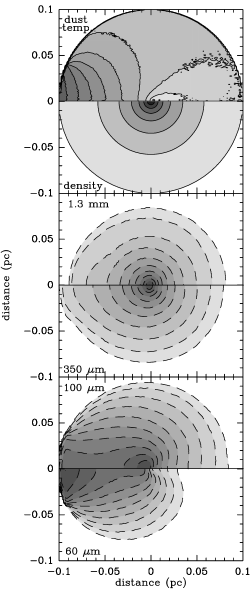
Figure 4: Model results for a spherical (Bonnor-Ebert) cloud core heated by the standard ISRF and a B3 star located at 0.15 pc from the surface of the cloud (on the left side in this figure). The core has central density $n({\rm H}_{2})=4.4\times 10^{6}$ cm^-3, gas temperature $T_{\rm g}=10$ K, and radius $R=0.1$ pc. The top panel shows the dust temperature (top half) and the density (bottom half). Isopycnic curves are logarithmically spaced by 0.5 and the boundary density is $n({\rm H}_{2})=2.3\times 10^{3}$ cm^-3. Isothermal curves are spaced by 2 K starting from $T_{\rm d}=14$ K. The middle and bottom panels show the emission at 1.3 mm, 350 $\mu$m, 100 $\mu$m and 60 $\mu$m. Isophotes are logarithmically spaced by 0.2 starting from $0.01\times I_{\nu}^{\rm max}$. The peak intensity $I_{\nu}^{\rm max}$ is 78 MJy sr^-1 at 1.3 mm, 3347 MJy sr^-1 at 350 $\mu$m, 1404 MJy sr^-1 at 100 $\mu$m and 200 MJy sr^-1 at 60 $\mu$m.

The resulting temperature distribution is shown in the top panel of Fig. 4. As expected, the cloud is hotter on the side facing the star, and the temperature decreases both radially and azimuthally, with the lowest temperature close to the centre of the core, which is almost twice higher than the minimum temperature of the Black ISRF heated core with the same density profile (Fig. 1). The ratio $L_{\ast}/L^{\rm ISRF}$ is $\sim 20$, and the inverse square dependence of $dL$ (see Eq. 13) that makes this ratio over a surface element be much larger close to the star, has the consequence that the isotropic ISRF is negligible almost everywhere. The exception to this is on the core’s side opposite to the star, where the shielding provided by the cloud’s center suffices to make the isotropic ISRF the dominant heating field.

In Fig. 4 we show the simulated emission maps at 1.3 mm, 350$\leavevmode\nobreak\ \mu$m, 100$\leavevmode\nobreak\ \mu$m and 60$\leavevmode\nobreak\ \mu$m. The 1.3 mm map shows slight distortions due to the temperature structure but clearly allows a reasonable determination of the mass distribution in the BE sphere. As one goes to shorter wavelengths however, the distortions become extreme and at 60 microns, one sees essentially the heated surface of the cloud. Thus maps at different wavelengths may allow the identification of a heating source and show where the star is along the line of sight relative to the cloud. In such situations, there will often be mid–IR data available which will additionally define the geometry of the “envelope” or PDR layer hypothesised in our analysis.

6 Three-dimensional models

Reverting to the case of an isotropic radiation field, we now consider the radiative transfer in a fully 3-D density distribution built on the results of Galli et al. (2001) for magnetized disks with uniform mass-to-flux ratio $M(\Phi)/\Phi$ (isopedic). A computationally convenient characteristic of these models is the existence of non-axisymmetric but analytical solutions of the equations of magnetostatics, corresponding to surface density distributions $\Sigma$ separable in polar coordinates $(\varpi,\varphi)$:

$$\Sigma(\varpi,\varphi)=\frac{\Theta a^{2}}{2\pi\epsilon G\varpi}S(\varphi),$$ (14)

where

$$S(\varphi)=\frac{\sqrt{1-e^{2}}}{1+e\cos\varphi},$$ (15)

with $0<e<1$. Here, $\Theta\geq 1$ and $\epsilon\leq 1$ represent the increase of gas pressure and the reduction of the gravitational constant due to magnetic pressure and magnetic tension, respectively, related to the nondimensional mass-to-flux ratio $\lambda=2\pi G^{1/2}M(\Phi)/\Phi$ by the relations (Shu & Li 1997)

$$\epsilon=1-\frac{1}{\lambda^{2}},\qquad\Theta=\frac{\lambda^{2}+3}{\lambda^{2}+1}.$$ (16)

We construct, in a rather ad hoc way, a 3-D model assuming a vertical stratification of gas in hydrostatic equilibrium and imposing the condition that the column density of the resulting density distribution reproduces Eq. (14), obtaining

$$\rho(\varpi,\varphi,z)=\frac{a^{2}\Theta^{2}}{8\pi\epsilon^{2}G\varpi^{2}}S^{2}(\varphi)\;{\rm sech}^{2}\left[\frac{z}{H(\varpi,\varphi)}\right],$$ (17)

where $H(\varpi,\varphi)=a^{2}/\pi G\Sigma(\varpi,\varphi)$.

As a specific example, we adopt the parameters derived by Galli et al. (2001) to match the thermal dust emission map obtained by Ward-Thompson et al. (1999) for the starless core L1544. We assume an effective sound speed $a=0.21$ km s^-1, a nondimensional mass-to-flux ratio $\lambda=2$, an eccentricity $e=0.54$, and we define the core boundary by the isopycnic surface $n({\rm H}_{2})=10^{4}$ cm^-3.

For this model we have also computed the gas temperature. To do this, we first notice that the energy deposited in the gas by cosmic ray ionization is negligible when compared to the energy absorbed by the dust, so that the energy transfer between gas and dust will not significantly affect the grain temperature. Therefore, it is only necessary to solve the equation of thermal equilibrium of the gas,

$$\Gamma_{\rm cr}-\Lambda_{\rm g}-\Lambda_{\rm gd}=0,$$ (18)

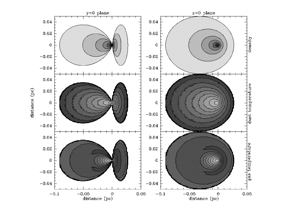
Figure 5: Density and temperature distribution in the magnetic 3-D model. Panels on the left (right) side show results in $y=0$ ($z=0$) plane, respectively. The top panels show the gas density, with isopycnic curves logarithmically spaced by 0.5, and density on the boundary $n({\rm H}_{2})=10^{4}$ cm^-3. The middle panels show the dust temperature distribution, with isothermal curves spaced by 1 K between the minimum (7 K) and maximum (14 K) values. The bottom panels show the gas temperature, with isothermal levels ranging from 7 to 14 K.

with ${\Gamma_{\rm cr}}$ the cosmic-ray heating rate, ${\Lambda_{\rm g}}$ the gas cooling rate by molecular and atomic transitions, and ${\Lambda_{\rm gd}}$ the gas-dust energy transfer rate. For these quantities, we assume the values given by Goldsmith (2001). We also assume a CO depletion factor of the form $f_{\rm dep}=\exp(n/n_{\rm dep})$, where the critical density for CO depletion is taken to be $n_{\rm dep}=5.5\times 10^{4}$ cm^-3. Fig. 5 shows the density, dust temperature and gas temperature of our model, with the left and right panels showing the $y=0$ and the $z=0$ plane, respectively.

This 3-D model and the 2-D toroidal model presented in the previous section show qualitatively similar temperature distributions, but the mismatch between isopycnic and dust isothermal surfaces is enhanced in the 3-D model, particularly in the $y=0$ plane where the geometry is more complex.

The gas temperature, as it depends on both the dust temperature and on the gas density, shows a different distribution from either (Fig. 5). At the dense center, the temperatures of the gas and the dust are well coupled, but they are decoupled at the lower density boundary. This results in a non-monotonic behaviour of the gas temperature, which reaches a maximum at intermediate density (an effect that also occurs in 1D geometry, as shown in Galli et al. 2002). It is also evident, from Fig. (5) that the gas temperature has a slightly higher value in the right side of the singularity than at the left, which is a consequence of the different dust temperature values at the density where the turnover in the gas temperature occurs on the two sides of the singularity.

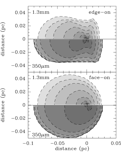
Figure 6: Normalized emission for the 3-D model, seen edge-on (top panel) and face-on (bottom panel). Each panel shows the emission at 1.3 mm (top half) and at 350 $\mu$m (bottom half). Isophotal curves are logarithmically spaced by 0.2 starting from the lower value $0.01\times I_{\nu}^{\rm max}$. With the adopted opacity law (OH5), the peak values are: $I_{\nu}^{\rm max}=89$ MJy sr^-1 at 1.3 mm and 460 MJy sr^-1 at 350 $\mu$m (edge-on case); $I_{\nu}^{\rm max}=72$ MJy sr^-1 at 1.3 mm and 307 MJy sr^-1 at 350 $\mu$m (face-on case).

Fig. 6 shows simulated dust emission maps at 1.3 mm and 350 $\mu$m for the side view and top view. The flattening towards the center due to the dust temperature gradient is evident from the comparison between the emission at the two wavelengths. The vertical density stratification has a fairly strong effect on the shape of the map seen from the side, but is not noticable from the top. In general, one notes a slight “bottleneck” deviation from a purely elliptical shape of the singular isothermal disk model present in Galli et al. (2001). We note also that the “cometary shape” of the edge-on 1.3 mm map is rather similar to that observed towards L1544 and L63 by Ward-Thompson et al. (1999).

7 Conclusions

In this paper we have presented a Monte Carlo model for radiative transfer applicable to the study of the physical conditions in starless molecular cloud cores. The method described is able to compute accurately and efficiently the dust and gas temperature distribution in clouds of specified but arbitrary density profiles heated by the ISRF, an external stellar source, or a combination thereof. In addition, the method allows the computation of synthetic maps of the emission at near-infrared and submillimeter wavelengths for arbitrary viewing angles, and to predict the emergent spectral energy distribution. We have successfully tested our code by detailed comparison with one-dimensional calculations in spherical symmetry (ZWG, Galli et al. 2002) and have shown that the assumption of effective optical thinness is a good one for prestellar cores. As preliminary applications of our code, we have considered the radiative transfer in model clouds of increasing degrees of asymmetry and in a spherical cloud core heated by a neighboring star.

With our method, we confirm the results of ZWG, Evans et al. (2001), and Stamatellos & Whitworth (2003) that the dust temperature in cloud models with physical characteristics typical of dense cores varies monotonically between a minimum value at the center (6–7 K) and a maximum value near the cloud’s edge (14–15 K) for the standard ISRF.

In general, maps at submillimeter wavelengths closely reproduce the column density distribution, even for the most non-isothermal configurations. In the Rayleigh-Jeans regime, in fact, temperature differences of a factor $\sim 2$ along the line-of-sight are washed out by the much larger variation of the density. However, the decrease of the dust temperature at the cloud center has the consequence that submillimeter maps sample preferentially the low-density envelope of prestellar cores, and are therefore unable to distinguish centrally peaked (pivotal) configurations from more flattened density profiles. We also note that our three-dimensional model based on the work of Galli et al. (2001) produces in natural fashion the cometary structure observed towards many prestellar cores.

For a spherical core heated by an external stellar source close to the cloud’s surface, the temperature distribution is non-spherical, but the submillimeter emission generally reproduces the core’s column density profile. Deviations from circular symmetry become extremely apparent on the other hand shortward of 100 $\mu$m where one samples mainly the heated surface layer.

Figure 1: Comparison of dust temperature profiles obtained with different methods for a BE sphere with central density $n({\rm H}_{2})=4.4\times 10^{6}$ cm^-3, gas temperature $T_{g}=12$ K, and radius $R=0.1$ pc. The solid and dotted curves shows the result obtained with the ray integration method of ZWG and the Monte Carlo code, without including the effects of re-emission. The two results are in excellent agreement. The short-dashed curve shows the dust temperature computed with the Monte Carlo code including re-emission. In all three cases the cloud has no envelope.

Figure 2: Dust temperature profiles (including re-emission) for the cloud model shown in Fig. 1 for different choices of the dust opacity: solid curve, OH1; dotted curve, OH4; short-dashed curve, OH5; long-dashed curve, OH8 (see text for the definitions). The gas-to-dust ratio was varied so that the total extinction at 2.2 $\mu$m is the same in all cases. The cloud is embedded in a spherical outer envelope with total extinction $A_{2.2\mu\rm{m}}^{\rm env}=0.1$.

- (1) André, P., Ward-Thompson, D., Barsony, M. 2000, in Protostars & Planets IV, eds. V. Mannings, A. P. Boss, & S. S. Russell, (Tucson, The University of Arizona Press), p. 59
- (2) André, P., Bouwman, J., Belloche, A., Hennebelle, P. 2003, in “Chemistry as a diagnostic of star formation” C. L. Curry & M. Fich, eds., in press
- (3) Bacmann, A. André, P., Puget, J.-L., et al. 2000, A&A, 361, 555
- (4) Bianchi, S., Gonçalves, J., Albrecht, M., Caselli, P., Chini, R., Galli, D., Walmsley, M. 2003, A&A, in press
- (5) Black, J. H. 1994, in The First Symposium on the Infrared Cyrrus and Diffuse Interstellar Clouds, ed. R. M. Cutri & W. B. Latter, ASP Conf. Ser., 58, 355
- (6) Bjorkman, J. E., Wood, K. 2001, ApJ, 554, 615
- (7) Basu, S. 2000, ApJ, 540, L103
- (8) Caselli, P., Walmsley, C. M., Zucconi A., et al. 2002a, ApJ, 565, 331
- (9) Caselli, P., Walmsley, C. M., Zucconi A., et al. 2002b, ApJ, 565, 344
- (10) Désert, F.-X., Boulanger, F., Puget, J. L. 1990, A&A, 237, 215
- (11) Evans, N. J., Rawlings, J. M. C., Shirley, Y., Mundy, L. G. 2001, ApJ, 557, 193
- (12) Galli, D., Shu, F. H., Laughlin, G., Lizano, S. 2001, ApJ, 551, 367
- (13) Galli, D., Walmsley, Gonçalves, J. 2002, A&A, 394, 275
- (14) Goldsmith, P. F. 2001, ApJ, 557, 763
- (15) Ivezic, Z., Groenewegen, M. A. T., Men’schikov, A., Szczerba, R. 1997, MNRAS, 291, 121
- (16) Jones, C. E., Basu, S. 2002, ApJ, 569, 280
- (17) Kramer, C., Richer, J., Mookerjea, B., Alves, J., Lada, C. 2003, A&A, 399, 1073
- (18) Leung, C. M. 1976 ApJ, 209, 75
- (19) Li, D., Goldsmith, P. F., Menten, K. 2003, ApJ, 587, 262
- (20) Li, Z.-Y., Shu, F. H. 1996, ApJ, 472, 211
- (21) Natta, A., Palla, F., Preite-Martinez, A., Panagia, N. 1981, A&A, 99, 289
- (22) Niccolini, G., Woitke, P., Lopez, B. 2003, A&A, 399, 703
- (23) Olofsson, H., Johansson, L. E. B., Hjalmarson, A., Nguyen-Quang-Rieu, Mr. 1982, A&A, 107, 128
- (24) Ossenkopf, V., Henning, T. 1994, A&A, 291, 943 (OH)
- (25) Rowan-Robinson, M. 1980, ApJS, 44, 403
- (26) Shirley, Y., Evans, N. J., Rawlings, J. M. C., Gregersen, E. M. 2000, ApJS, 131, 249
- (27) Shu, F. H., Adams, F. C., Lizano, S. 1987, ARA&A, 25, 31
- (28) Shu, F. H., Li, Z.-Y. 1997, ApJ, 475, 251
- (29) Spagna, G. F. Jr., Leung, C. M., Egan, M., P. 1991, ApJ, 379, 232
- (30) Stamatellos, D., Whitworth, A. P. 2003, A&A, in press
- (31) Tafalla, M., Myers, P. C., Caselli, P., Walmsley, C. M., Comito, C. 2002, ApJ, 565, 331
- (32) Ward-Thompson, D., Motte, F., André, P. 1999, MNRAS, 305, 143
- (33) Ward-Thompson, D., Kirk, J. M., Crutcher, R. M., Greaves, J. S., Holland, W. S., André, P. 2000, ApJ, 537, L35
- (34) Ward-Thompson, D., André, P., Kirk, J. M. 2002, MNRAS, 329, 257
- (35) Wolf, S., Henning, Th, Stecklum, B. 1999, A&A, 349, 839
- (36) Zucconi, A., Walmsley, C. M., Galli, D. 2001, A&A, 376, 650 (ZWG)