TESTING CIRCUIT MODELS FOR THE ENERGIES OF CORONAL MAGNETIC FIELD CONFIGURATIONS

Abstract

Circuit models involving bulk currents and inductances are often used to estimate the energies of coronal magnetic field configurations, in particular configurations associated with solar flares. The accuracy of circuit models is tested by comparing calculated energies of linear force-free fields with specified boundary conditions with corresponding circuit estimates. The circuit models are found to provide reasonable (order of magnitude) estimates for the energies of the non-potential components of the fields, and to reproduce observed functional dependences of the energies. However, substantial departure from the circuit estimates is observed for large values of the force-free parameter, and this is attributed to the influence of the non-potential component of the field on the path taken by the current.

Appl. Opt.

1 Introduction

Solar flares are understood to involve the conversion of magnetic energy in the solar corona into the energy of particles and radiation. In particular flare energy is believed to derive from non-potential coronal magnetic fields, i.e. that part of the magnetic field produced by currents flowing in the solar corona (e.g. Tandberg-Hanssen and Emslie, 1988).

The origin of flare energy in coronal currents has suggested to many authors the use of a circuit analogy (e.g. Alfvén and Carlqvist 1967; Spicer, 1982; Somov 1992; Melrose, 1995; Melrose 1997; Longcope and Noonan 2000; Khodachenko and Zaitsev, 1998; Khodachenko, Haerendel and Rucker, 2003). It is well known that the energy of a system of $N$ distinct current-carrying circuits may be written (e.g. Jackson, 1998)

$$E=\frac{1}{2}\sum_{i=1}^{N}L_{i}I_{i}^{2}+\sum_{i=1}^{N}\sum_{j>i}M_{ij}I_{i}I_{j},$$ (1)

where

$$L_{i}=\frac{\mu_{0}}{4\pi I_{i}^{2}}\int_{C_{i}}d^{3}x_{i}\int_{C_{i}}d^{3}x_{i}^{\prime}\frac{{\bf J}({\bf x}_{i})\cdot{\bf J}({\bf x}_{i}^{\prime})}{|{\bf x}_{i}-{\bf x}_{i}^{\prime}|}$$ (2)

is the self-inductance and

$$M_{ij}=\frac{\mu_{0}}{4\pi I_{i}I_{j}}\int_{C_{i}}d^{3}x_{i}\int_{C_{j}}d^{3}x_{j}^{\prime}\frac{{\bf J}({\bf x}_{i})\cdot{\bf J}({\bf x}_{j}^{\prime})}{|{\bf x}_{i}-{\bf x}_{j}^{\prime}|}$$ (3)

is the mutual inductance, and where ${\bf J}({\bf x})$ is the current density at a point ${\bf x}$ in space, and $C_{i}$ is the volume of the $i^{\rm th}$ circuit. Although Equations (1)—(3) are quite general, their utility relies on having a small number of well-defined circuits with simple geometries for which analytic expressions for $L_{i}$ and $M_{ij}$ may be evaluated, and in particular for which $L_{i}$ and $M_{ij}$ are independent of $I_{i}$ and $I_{j}$. This is the situation for currents flowing in a small number of “wire” loops, i.e. loops with a fixed geometry. Circuit models for coronal magnetic fields adopt wire loop configurations. For example, in the flare model of Melrose (1997) based on reconnection between current-carrying magnetic flux tubes, each flux tube is represented by fixed toroidal structures carrying a uniform axial current. The self-inductance of such a structure is (e.g. Landau and Lifshitz, 1960)

$$L_{i}=\mu_{0}a_{i}C_{i},\quad\quad C_{i}=\ln\frac{8a_{i}}{r_{i}}-\frac{7}{4},$$ (4)

where $a_{i}$ is the major radius of the toroid and $r_{i}$ is the minor radius. Melrose (1997) also adopts the following approximate expression for the mutual inductance between two loops whose centres are separated by a distance $d_{ij}$ and whose axes subtend an angle $\theta_{ij}$:

$$M_{ij}=\mu_{0}\frac{8a_{i}^{2}a_{j}^{2}(C_{i}C_{j})^{1/2}\cos\theta_{ij}}{\left[(a_{i}+a_{j})^{2}+d_{ij}^{2}\right]^{3/2}}.$$ (5)

This formula is not exact but is based on interpolation between known results. An exact formula which holds for two axially-aligned line-current loops separated by a distance $d_{ij}$ is (Stratton, 1941)

$$M_{ij}=\mu_{0}(a_{i}a_{j})^{1/2}\left[\left(\frac{2}{k_{ij}}-k_{ij}\right)K(k_{ij})-\frac{2}{k_{ij}}E(k_{ij})\right],$$ (6)

where

$$\quad k_{ij}^{2}=\frac{4a_{i}a_{j}}{(a_{i}+a_{j})^{2}+d_{ij}^{2}},$$ (7)

and where $K(x)$ and $E(x)$ are complete elliptic integrals.

Real coronal currents do not flow along simple wire loops — they are distributed in the coronal volume, and describe complicated paths. A common model for current-carrying coronal fields is the force-free model, in which the magnetic field ${\bf B}$ satisfies ${\bf J}\times{\bf B}=0$, (as well as $\nabla\cdot{\bf B}=0$) where ${\bf J}=\frac{1}{\mu_{0}}\nabla\times{\bf B}$. In other words the current density is everywhere parallel to the magnetic field. Unfortunately the force-free field equation is in general nonlinear and hence difficult to solve. A restricted set of force-free fields — linear force free fields — are easy to calculate (e.g. Nakagawa and Raadu 1972; Chiu and Hilton 1977; Alissandrakis, 1981; Gary, 1989). For these fields $\nabla\times{\bf B}=\alpha{\bf B}$ where $\alpha$ is a constant, the force-free parameter. Linear force-free models for coronal magnetic fields permit detailed descriptions of current paths in the corona, although they have limitations as large scale models for solar fields (e.g. Sturrock, 1994).

In this paper the accuracies of simple circuit models for coronal magnetic field energies are tested by application to linear force-free field configurations. To our knowledge this is the first quantitative test of the accuracy of the circuit model in the solar context. For simplicity, the comparison is limited to field configurations representing one and two magnetic loops. The order of presentation is as follows. In § 2 the method is outlined, including the adopted boundary conditions (§ 2.1), and the details of the linear force-free (§ 2.2) and circuit (§ 2.3) models. In § 3 the results of the calculations for one loop (§ 3.1) and two loops (§ 3.2) are presented. Finally in § 4 the results are discussed.

2 Method

2.1 Boundary conditions

The plane $z=0$ is taken to represent the photosphere, and the half space above this plane ($z>0$) represents the coronal volume. We consider simple boundary field configurations suggestive of one coronal loop:

$$B_{z}(x,y,0)=B_{1}\exp\left[-\frac{({\bf x}-{\bf x}_{1+})^{2}}{2\sigma_{1}^{2}}\right]-B_{1}\exp\left[-\frac{({\bf x}-{\bf x}_{1-})^{2}}{2\sigma_{1}^{2}}\right],$$ (8)

and two coronal loops:

$$B_{z}(x,y,0) = B_{1}\exp\left[-\frac{({\bf x}-{\bf x}_{1+})^{2}}{2\sigma_{1}^{2}}\right]-B_{1}\exp\left[-\frac{({\bf x}-{\bf x}_{1-})^{2}}{2\sigma_{1}^{2}}\right]$$ (9)

$$+ B_{2}\exp\left[-\frac{({\bf x}-{\bf x}_{2+})^{2}}{2\sigma_{2}^{2}}\right]-B_{2}\exp\left[-\frac{({\bf x}-{\bf x}_{2-})^{2}}{2\sigma_{2}^{2}}\right],$$

respectively, where ${\bf x}=x\hat{\bf x}+y\hat{\bf y}$. The positions ${\bf x}_{1\pm}$ and ${\bf x}_{2\pm}$ define the loop footpoints.

It is convenient to adopt non-dimensional units in which lengths are expressed in terms of a basic length $L$, and magnetic fields are expressed in terms of the peak vertical field $B_{1}$ at the base of loop one, e.g.

$$x=L\overline{x},\quad B_{z}=B_{1}\overline{B}_{z},\quad{\rm etc.},$$ (10)

where bars indicate dimensionless versions of quantities.

2.2 Linear force-free model

A solution to the linear force-free equations is provided by (e.g. Alissandrakis, 1981)

$$b_{x}(u,v,\overline{z}) = \frac{-i(uk-v\overline{\alpha})}{2\pi(u^{2}+v^{2})}e^{-k\overline{z}}b_{z}^{0}(u,v),$$

$$b_{y}(u,v,\overline{z}) = \frac{-i(vk+u\overline{\alpha})}{2\pi(u^{2}+v^{2})}e^{-k\overline{z}}b_{z}^{0}(u,v),$$

$$b_{z}(u,v,\overline{z}) = e^{-k\overline{z}}b_{z}^{0}(u,v),$$ (11)

where $b_{i}(u,v,\overline{z})$ denotes the Fourier transform of $\overline{B}_{i}(\overline{x},\overline{y},\overline{z})$ in $\overline{x}$ and $\overline{y}$ ($u$ and $v$ are the wavenumbers corresponding to $\overline{x}$ and $\overline{y}$ respectively), $b_{z}^{0}(u,v)=b_{z}(u,v,0)$ is the Fourier transform of $\overline{B}_{z}(\overline{x},\overline{y},0)$, $\overline{\alpha}=\alpha L$ is the force-free parameter, and

$$k=\left[4\pi^{2}(u^{2}+v^{2})-\overline{\alpha}^{2}\right]^{1/2}.$$ (12)

Equation (2.2) requires $(u^{2}+v^{2})^{1/2}\geq|\overline{\alpha}|/(2\pi)$. Since large $u$ and $v$ correspond to variation on small spatial scales, this solution is termed the “small scale solution” to the linear force-free field equations. Of course, inversion of this solution in Fourier space involves integration over all $u$ and $v$. The small scale solution only provides a solution matching given boundary conditions $\overline{B}_{z}(\overline{x},\overline{y},0)$ if $b_{z}^{0}(u,v)$ is identically zero for $(u^{2}+v^{2})^{1/2}<|\overline{\alpha}|/(2\pi)$. In general this is not true, and in particular it will not be true for the boundary conditions (8) and (9), for any given $\overline{\alpha}\neq 0$ [although $b_{z}^{0}(u,v)$ is expected to be small for small $u$ and $v$, and identically zero for $u=v=0$ provided the net flux is zero]. In the following we effectively calculate $b_{z}^{0}(u,v)$ for the given boundary conditions and then impose $b_{z}^{0}(u,v)=0$ for $(u^{2}+v^{2})^{1/2}<|\overline{\alpha}|/(2\pi)$.

The physical justification for considering only the small scale solution is that it provides a linear force-free field with finite energy. Following Alissandrakis (1981) and Gary (1989), using Parseval’s theorem the energy of the linear force-free field (2.2) in the half space $\overline{z}>0$ is

$$\overline{E}_{F}=\int_{-\infty}^{\infty}du\int_{-\infty}^{\infty}dv\frac{|b_{z}^{0}(u,v)|^{2}}{\left[4\pi^{2}(u^{2}+v^{2})-\overline{\alpha}^{2}\right]^{1/2}}.$$ (13)

Once again this expression requires the Fourier components $b_{z}^{0}(u,v)$ to be identically zero for $u$ and $v$ such that $(u^{2}+v^{2})^{1/2}<|\overline{\alpha}|/(2\pi)$. The large scale components of the field have infinite energy, and in this sense the general linear force-free boundary value problem has no physical solution (Alissandrakis, 1981). In practice we use the Fast Fourier Transform (FFT) of the boundary field defined on an $N$ by $N$ grid over the region $0\leq\overline{x}\leq 1$, $0\leq\overline{y}\leq 1$. The smallest non-zero wavenumber that is determined from these ‘observations’ of the field (by analogy with magnetograph observations) is $u_{\rm min}=v_{\rm min}=1-1/N$. It follows that the energies determined from the discrete counterpart of (13) are finite for all $N$ provided $|\overline{\alpha}|<\overline{\alpha}_{\rm max}=2\pi$.

Finally we note that the variation of (13) with $\overline{\alpha}$ for small values of the force-free parameter is made obvious by a binomial expansion:

$$\overline{E}_{F}(\overline{\alpha})=\overline{E}_{F}(0) + \frac{\overline{\alpha}^{2}}{16\pi^{3}}\int\!\!\int\frac{|b_{z}^{0}(u,v)|^{2}}{(u^{2}+v^{2})^{3/2}}dudv$$ (14)

$$+ \frac{3\overline{\alpha}^{4}}{256\pi^{5}}\int\!\!\int\frac{|b_{z}^{0}(u,v)|^{2}}{(u^{2}+v^{2})^{5/2}}dudv+\cdots.$$

Hence for small $\overline{\alpha}$ the non-potential component of the field scales with $\overline{\alpha}^{2}$.

2.3 Circuit model

The current in a loop in the circuit model is taken to be the axial current contained within a radius $\overline{R}$ of the centre of a footpoint:

$$\overline{I}_{1} = 2\pi\int_{0}^{\overline{R}}\overline{J}_{z}\overline{r}\,d\overline{r}$$ (15)

$$\approx 2\pi\overline{\alpha}\overline{\sigma}_{1}^{2}\left(1-e^{-\overline{R}^{2}/(2\overline{\sigma}_{1}^{2})}\right),$$

using the boundary conditions (8) or (9), and assuming that the footpoints are well separated. Similarly

$$\overline{I}_{2}\approx 2\pi\overline{\alpha}\beta\overline{\sigma}_{2}^{2}\left(1-e^{-\overline{R}^{2}/(2\overline{\sigma}_{2}^{2})}\right),$$ (16)

where $\beta\equiv B_{2}/B_{1}$, and $\overline{J}_{z}=\mu_{0}LJ_{z}/B_{1}$.

The energy of the single loop model in the half space $\overline{z}>0$ is then estimated using (4):

$$\overline{E}_{C}=\frac{1}{2}\overline{L}_{1}\overline{I}_{1}^{2},$$ (17)

where

$$\overline{L}_{1}=\overline{a}_{1}\overline{C}_{1},\quad{\rm with}\quad\overline{C}_{1}=\ln(8\overline{a}_{1}/\overline{R})-7/4.$$ (18)

Similarly the energy of the two loop system can be expressed as

$$\overline{E}_{C}=\frac{1}{2}\overline{L}_{1}\overline{I}_{1}^{2}+\frac{1}{2}\overline{L}_{2}\overline{I}_{2}^{2}+\overline{M}_{12}\overline{I}_{1}\overline{I}_{2},$$ (19)

where $\overline{M}_{12}$ is the mutual inductance. For the general case (loop major radii $\overline{a}_{1}$, $\overline{a}_{2}$, minor radii $\overline{r}_{1}$, $\overline{r}_{2}$, centres separated by $\overline{d}_{12}$, and axes oriented at an angle $\theta_{12}$) the non-dimensional version of the interpolating formula Equation (5) from Melrose (1997) may be used:

$$\overline{M}_{12}=\frac{8\overline{a}_{1}^{2}\overline{a}_{2}^{2}(\overline{C}_{1}\overline{C}_{2})^{1/2}\cos\theta_{12}}{\left[(\overline{a}_{1}+\overline{a}_{1})^{2}+\overline{d}_{12}^{2}\right]^{3/2}}.$$ (20)

For the more restricted case of line-current loops with their axes aligned ($\theta_{12}=0$) the non-dimensional version of the exact Equation (6) may be used:

$$\overline{M}_{12}=\mu_{0}(\overline{a}_{1}\overline{a}_{2})^{1/2}\left[\left(\frac{2}{\overline{k}_{12}}-\overline{k}_{12}\right)K(\overline{k}_{12})-\frac{2}{\overline{k}_{12}}E(\overline{k}_{12})\right],$$ (21)

where

$$\quad\overline{k}_{12}^{2}=\frac{4\overline{a}_{1}\overline{a}_{2}}{(\overline{a}_{1}+\overline{a}_{2})^{2}+\overline{d}_{12}^{2}}.$$ (22)

3 Results

3.1 One loop

Figure 1 illustrates a single loop configuration, for the boundary conditions $\overline{{\bf x}}_{1+}=(0.5,0.1)$, $\overline{{\bf x}}_{1-}=(0.5,-0.1)$, $\overline{\sigma}_{1}=0.05$, and $\overline{\alpha}=1$. (These values are adopted as nominal values.) To construct this figure, the linear force-free field corresponding to (2.2) was calculated [using the FFT of Equation (8)] on a $128\times 128\times 64$ grid corresponding to the region $0\leq\overline{x}\leq 1$, $0\leq\overline{y}\leq 1$, $0\leq\overline{z}\leq 1$. Field lines were traced for points at a radius $\overline{\sigma}_{1}/2=0.025$ from the positive footpoint.

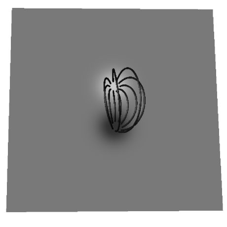
Figure 1: A single loop configuration.

The free energy $\overline{E}_{F}(\overline{\alpha})-\overline{E}_{F}(0)$ of the field can be estimated by taking the FFT of the boundary field with $N$ gridpoints and then evaluating the integral (13) using the trapezoidal rule. We label this estimate $W_{N}$. Figure 2 shows how the result depends on $N$, for the nominal choices of $\overline{{\bf x}}_{1\pm}$, $\overline{\sigma}_{1}$, and $\overline{\alpha}$. The upper panel plots $W_{N}$ versus $N$, for $N=32,64,128,...,4096$. The lower panel plots $W_{N}/W_{N/2}-1$ versus $N$ as a log-log plot. A condition for the sequence of values of $W_{N}$ to converge is that $W_{N}/W_{N/2}$ approaches unity as $N\rightarrow\infty$. The lower panel suggests that this is occurring, and moreover $W_{N}/W_{N/2}-1\sim N^{-1}$. For the calculations in the paper we have used $N=512$. The estimates of $W_{N}$ for $N=512$ and $N=4096$ differ by about $0.5\%$, which suggests that $N=512$ is sufficiently accurate for present purposes.

Figure 2: Upper: Variation of the free energy estimate $W_{N}$ with $N$, for the single loop configuration. Lower: Convergence of the estimates.

The first question to be addressed is the variation of the energy estimates with $\overline{I}_{1}$. To vary $\overline{I}_{1}$ we have varied $\overline{\alpha}$, while keeping $\overline{\sigma}_{1}$ fixed [see Equation (15)]. We have also chosen $\overline{R}=\overline{\sigma}_{1}$, and used the nominal values of $\overline{{\bf x}}_{1\pm}$ and $\overline{\sigma}_{1}$. The field estimate of the energy $W_{512}$ and the circuit estimate $E_{C}$ were calculated for 50 values of $\overline{\alpha}$ between $0.001\overline{\alpha}_{\rm max}$ and $0.99\overline{\alpha}_{\rm max}$, with the values being equally spaced logarithmically. The results are plotted in Figure 3. The diamonds show the values of $W_{512}$ and the crosses show the values of $E_{C}$. The vertical dashed line is $\overline{\alpha}_{\rm max}$ and the horizontal dashed line is the estimate of $\overline{E}_{F}(0)$, the energy of the potential component of the field. The energy estimates for the non-potential component of the field and the circuit energy estimates are generally much smaller than the energy of the potential component of the field. The energy estimates for the non-potential component of the field exhibit a $\overline{I}_{1}^{2}$ dependence ($\overline{\alpha}^{2}$ dependence) for most of the chosen range, but increase more rapidly for large $\overline{I}_{1}$ ($\overline{\alpha}$). This functional dependence is consistent with Equation (14). The field and circuit energy estimates are within a factor of two of one another for most of the chosen range, but are out by more than a factor of 10 close to the maximum value of $\overline{\alpha}$. There is a simple physical interpretation for the observed dependence of the field energy on $\overline{I}$. For small values of the current the field associated with the current is small, and the magnetic field is dominated by the potential component. The current essentially follows the fieldlines of the potential field, i.e. there is a fixed geometrical path for the current. In this case the self-inductance defined by Equation (2) is independent of the current. For larger values of the current this is no longer the case: the field due to the current becomes comparable to the potential component of the field, and the path that the current takes then depends on the current. In particular, larger currents will tend to produce longer current paths, so the effective self-inductance will increase with current. In other words Equation (2) increases with current.

Figure 3: Current dependence of energy estimates for the single loop configuration.

Another question is the dependence of energy on the geometry of the loop. The major radius $\overline{a}$ was varied between 0.05 and 0.25 for the nominal choices of the other parameters, and Figure 4 shows the results. The energy estimates $W_{512}$ were divided by $\frac{1}{2}\overline{I}_{1}^{2}$ [see Equation (4)] to produce effective self-inductances, which are shown by diamonds. Results are shown for $\overline{\alpha}=1.0$ and $\overline{\alpha}=2.0$ — the effective self-inductances for the larger value of $\overline{\alpha}$ are slightly larger, for all values of major radius. The self-inductances $\overline{L}_{1}$ are indicated by crosses. This figure shows that the non-potential component of the field energy varies with major radius in a manner similar to that expected from the circuit model for the chosen range of values. The inferred self-inductance increases monotonically, as expected on the basis of the increase in area under the loop. However the precise functional dependence of the inferred self-inductance is somewhat different from that expected from the simple model $\overline{L}_{1}$. The similar results for the different values of $\overline{\alpha}$ show that the inferred self-inductance is almost independent of the value of the current, as expected on the basis of the argument given above.

Figure 4: Major radius dependence of self-inductance for the single loop configuration.

The minor radius dependence of energy was also examined. Figure 5 shows the effective self-inductance associated with the non-potential component of the magnetic field (diamonds) for $\overline{\sigma}_{1}$ between 0.01 and 0.1, and for the nominal values of the other parameters. The values of $\overline{L}_{1}$ are also plotted (crosses). This figure shows that the variation of the magnetic field energy with $\overline{\sigma}_{1}$ is qualitatively consistent with the circuit model. The effective self-inductance decreases with $\overline{\sigma}_{1}$, as expected from the decrease in area within within the loop as the minor radius of the loop increases.

Figure 5: Minor radius dependence of self-inductance for the single loop configuration.

3.2 Two loops

Figure 6 illustrates a particular two-loop configuration, for the boundary conditions $\overline{{\bf x}}_{1+}=(0.25,0.575)$, $\overline{{\bf x}}_{1-}=(0.25,0.425)$, $\overline{{\bf x}}_{2+}=(0.825,0.5)$, $\overline{{\bf x}}_{2-}=(0.675,0.5)$, $\overline{\sigma}_{1}=\overline{\sigma}_{2}=0.025$, $\beta=1$, and $\overline{\alpha}=1$. These choices correspond to loops with major radii $\overline{a}_{1}=\overline{a}_{2}=0.075$, with a distance $\overline{d}=0.5$ between their centres, and with axes at right angles to one another ($\theta_{12}=\pi/2$).

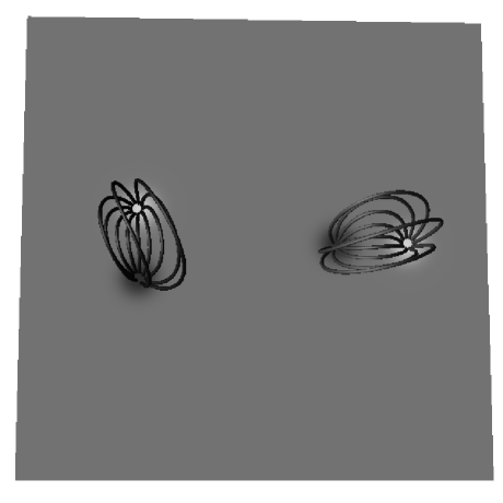
Figure 6: A two-loop configuration with $\theta_{12}=\pi/2$.

There are many energy dependences which could be investigated for two-loop configurations. However, from the point of view of the circuit model the interest is with the energy associated with the interaction between the loops, described by the mutual inductance. The interaction energy is determined in the following way. The field energy $W_{512}$ for the two loops is calculated. Then the field energy $W_{512,1}$ for loop one is calculated (the free energy of the small scale linear force-free field with the boundary conditions of loop one). Similarly the field energy $W_{512,2}$ for loop two is calculated. The energy $W_{512}-W_{512,1}-W_{512,2}$ is the interaction energy. Dividing this quantity by $\overline{I}_{1}\overline{I}_{2}$ defines an effective mutual inductance $\overline{M}_{12}^{\rm eff}$, which may be compared with circuit estimates.

First we consider a comparison with the Stratton (1941) formula (21), since it is an exact expression for mutual inductance (albeit for line currents). Recall that it is applicable only to the case of loops with aligned axes ($\theta_{12}=0$). The dependence of the mutual inductance on the major radius of loop two was investigated for loop parameters $\overline{a}_{1}=0.075$, $\overline{d}=0.5$, $\overline{\sigma}_{1}=\overline{\sigma}_{2}=0.025$, $\theta_{12}=0$, $\beta=1$, $\overline{\alpha}=1$, with the major radius of loop two taking 20 values in the range $0.02$ to $0.2$. Figure 7 shows the results. The points marked by diamonds are the mutual inductances calculated for the field following the procedure outlined above. The points marked with crosses are the mutual inductances given by the formula (21). The inferred mutual inductances are qualitatively consistent with the circuit values, and a similar functional dependence is observed.

Figure 7: Variation of effective inductance with major radius of loop 2 for the two-loop configuration, and comparison with the Stratton (1941) formula.

Next we examine the Melrose (1997) interpolation formula (20), which is more general than the Stratton (1941) formula, but is approximate. We considered a two-loop configuration with fixed parameters but with different values of $\theta_{12}$, corresponding to a rotation of loop two with respect to loop one. Specifically the values $\overline{a}_{1}=\overline{a}_{2}=0.075$, $\overline{d}=0.5$, $\overline{\sigma}_{1}=\overline{\sigma}_{2}=0.025$, $\beta=1$, and $\overline{\alpha}=1$ were chosen, together with 21 values of $\theta_{12}$ in the range $0\leq\theta_{12}\leq\pi$. Figure 8 shows the results. The crosses are the circuit values. Following Equation (20) the circuit model exhibits a simple cosine dependence on $\theta_{12}$, and in particular is zero for $\theta_{12}=\pi/2$, because perpendicular loops have no flux linkage. The diamonds are the values of $\overline{M}_{12}^{\rm eff}$ determined following the procedure outlined above. The observed functional dependence is essentially cosine, and indeed the effective mutual inductance is very close to zero for $\theta_{12}=\pi/2$. However, the values of $\overline{M}_{12}^{\rm eff}$ are considerably larger than the values given by the Melrose formula: the ratio of the values is close to eight over the range of $\theta_{12}$. This figure also shows the mutual inductance obtained using the Stratton (1941) formula for the special case $\theta_{12}=0$ as an asterisk. The Stratton value is slightly larger than $\overline{M}_{12}^{\rm eff}$ for $\theta_{12}=0$, and is considerably larger than the Melrose value. It is notable that the Melrose value differs from the Stratton value by more than an order of magnitude in this case.

Figure 8: Variation of effective inductance with angle between loops for the two-loop configuration, and comparison with the Melrose (1997) formula.

4 Discussion and conclusions

In this paper calculated energies of non-potential components of linear force-free fields are compared with simple circuit model estimates, for boundary conditions suggestive of one and two magnetic loops. The motivation is to test the circuit models, which are often invoked to estimate coronal magnetic field energies. In particular circuit models have been used to describe flare-related energy changes. In the Melrose (1997) model, preferred magnetic configurations for flaring are identified on the basis of geometrical dependences of circuit energy estimates.

In § 3.1 results for a single loop configuration are presented. An important result is the $\overline{\alpha}$-dependence of the energy of the non-potential component of the field. For a range of small values of the force-free parameter $\overline{\alpha}$ the free energy is found to be proportional to $\overline{\alpha}^{2}$, or equivalently to be proportional to the square of the current in the loop, consistent with the circuit model. This result is explained mathematically in terms of the $\overline{\alpha}^{2}$ dependence of the free energy appearing in Equation (14) for small $\overline{\alpha}$. For larger values of current (or $\overline{\alpha}$) the free energy increases more rapidly than the circuit prediction. This result is also expected for the two-loop configuration, since Equation (14) applies for any boundary conditions. A simple physical interpretation of this result is as follows. For small values of $\overline{\alpha}$ the non-potential component of the field is small compared to the potential component, and the current essentially follows the fieldlines of the potential field. Hence as $\overline{\alpha}$ is varied the geometry of the current does not change and the inductances [which are geometrical quantities — see Equations (2) and (3)] are constant. This situation corresponds to the free energy scaling with the square of the current (or $\overline{\alpha}^{2}$). For larger values of $\overline{\alpha}$ the non-potential component of the field becomes comparable to the potential component, and influences the path of the current. In this case the geometry [and hence the inductances as defined by Equations (2) and (3)] depend on $\overline{\alpha}$, which corresponds to the free energy scaling with a higher power of $\overline{\alpha}$. Although demonstrated here for a class of linear force-free fields, this effect is expected to be quite general and to limit the accuracy of simple circuit models in application to any force-free field for large values of current.

In § 3.1 the dependence of the free energy of the field on the geometry of the loop is also investigated (for a modest value of $\overline{\alpha}$). The functional dependences on minor radius and major radius are found to be qualitatively consistent with the circuit model.

Section § 3.2 presents the results for the two-loop configuration. The interaction energy of the two loops is obtained by calculating the free energy of the loops together and then subtracting off the individual free energies of each loop. This procedure is used to calculate an effective mutual inductance $\overline{M}_{12}^{\rm eff}$ for the field. This was then compared with simple circuit model formulae, namely an exact expression for the mutual inductance of two axially-aligned line-current loops due to Stratton (1941), and an approximate expression for the mutual inductance of oblique loops with finite cross section due to Melrose (1997). The Stratton formula is found to qualitatively reproduce the observed variation of $\overline{M}_{12}^{\rm eff}$ with the major radius of one loop. The Melrose formula is compared with $\overline{M}_{12}^{\rm eff}$ as one loop is rotated with respect to the other. The effective mutual inductance of the field reproduces the cosine dependence in the Melrose formula, and in particular the inferred mutual inductance is close to zero for the case of perpendicular loops. However, the calculated values of $\overline{M}_{12}^{\rm eff}$ are almost an order of magnitude larger than the Melrose formula values. Comparison with the Stratton formula for the case of parallel loops confirms that, for the chosen parameters, the Melrose formula underestimates the actual interaction energy. The Melrose expression is an interpolation between known results, and so the discrepancy can be attributed to the approximate nature of the formula.

In this paper linear force-free fields have been used because they are straightforward to calculate. It is likely that real coronal magnetic fields involve currents that are spatially highly concentrated, and hence require a nonlinear force-free model (or a description involving non-zero pressure forces). In this case circuit models may provide quite accurate energy estimates because the configuration closely resembles a set of isolated circuits. However, it is also possible that in the nonlinear case the current path sensitively depends on the value of the current, in particular for large currents, and this may limit the accuracy of simple circuit models, as discussed above.

Another point to note is that circuit models are really only useful if there are a small number of circuits which are easily identified. In this paper we have considered widely separated magnetic structures, which as a result have simple connectivity. In general coronal fields have a complicated topology, and it may be difficult to identify coronal current paths.

Circuit models appear to provide reasonably accurate free energy estimates for coronal magnetic field configurations for a range of values of the current, and also qualitatively describe various functional dependences of the free energy (the dependence on loop major radii, the dependence on the angle between two loops, etc.). Simple circuit models are less accurate for very large values of the current, when the current path depends on the value of the current. Despite this reservation, the results of this paper confirm the general utility of circuit models, in particular in their application to the flare phenomenon.

References

- Alfvén and Carlqvist (1967) Alfvén, H. and Carlqvist, P.: 1967, Sol. Phys., 1, 220.
- Alissandrakis (1981) Alissandrakis, C.E.: 1981, Astron. Astrophys., 100, 197.
- [missing (missing) Chiu, Y.T., and Hilton, H.H. 1977, Astrophys. J., 212, 873.
- Gary (1989) Gary, G.A.: 1989, Astrophys. J. Supp., 69, 323.
- Jackson (1998) Jackson, J.D.: 1998, Classical Electrodynamics, 3rd ed., John Wiley, New York.
- (6) Khodachenko, M., Haerendel, G., and Rucker, H.O.: 2003, Astron. Astrophys., 401, 721.
- Khodachenko and Zaitsev (1998) Khodachenko, M.L. and Zaitsev, V.V.: 1998, Astron. Rep., 42, 265.
- Landau and Lifshitz (1960) Landau, L.D. and Lifshitz, E.M.: 1960, Electrodynamics of Continuous Media, Pergamon, Oxford.
- Longcope and Noonan (2000) Longcope, D.W. and Noonan, E.J.: 2000, Astrophys. J., 542, 1088.
- Melrose (1995) Melrose, D.B.: 1995, Astrophys. J., 451, 391.
- Melrose (1997) Melrose, D.B.: 1997, Astrophys. J., 486, 521.
- Nakagawa and Raadu (1972) Nakagawa, Y. and Raadu, M.A.: 1972, Sol. Phys., 25, 127
- Somov (1992) Somov, B.V.: 1992, Physical Processes in Solar Flares, Kluwer, Dordrecht.
- Spicer (1982) Spicer, D.S.: 1982, Space Sci. Rev., 31, 351.
- Sturrock (1994) Sturrock, P.A.: 1994, Plasma Physics, Cambridge University Press, Cambridge
- Stratton (1941) Stratton, J.A.: 1941, Electromagnetic Theory, McGraw-Hill, New York
- Tandberg-Hanssen and Emslie (1988) Tandberg-Hanssen, E. and Emslie, A.G.: 1988, The Physics of Solar Flares, Cambridge University Press, Cambridge.