Mapping the Cosmic Web with Ly$\alpha$ Emission

Abstract

We use a high-resolution cosmological simulation to predict the distribution of H I Ly$\alpha$ emission from the low-redshift ($z\lesssim 0.5$) intergalactic medium (IGM). Our simulation can be used to reliably compute the emission from optically thin regions of the IGM but not that of self-shielded gas. We therefore consider several models that bracket the expected emission from self-shielded regions. Most galaxies are surrounded by extended ($\gtrsim 10^{2}\mbox{ kpc}$) “coronae” of optically thin gas with Ly$\alpha$ surface brightness close to the expected background. Most of these regions contain smaller cores of dense, cool gas. Unless self-shielded gas is able to cool to $T<10^{4.1}\mbox{ K}$, these cores are much brighter than the background. The Ly$\alpha$ coronae represent “cooling flows” of IGM gas accreting onto galaxies. We also estimate the number of Ly$\alpha$ photons produced through the reprocessing of stellar ionizing radiation in the interstellar medium of galaxies; while this mechanism is responsible for the brightest Ly$\alpha$ emission, it occurs on small physical scales and can be separated using high-resolution observations. In all cases, we find that Ly$\alpha$ emitters are numerous (with a space density $\sim 0.1\,h^{3}\mbox{ Mpc}^{-3}$) and closely trace the filamentary structure of the IGM, providing a new way to map gas inside the cosmic web.

1. Introduction

One of the most striking images to emerge from cosmological simulations is the “cosmic web”. Matter collapses into a web of moderately overdense sheets and filaments, with galaxies and galaxy clusters forming through continued collapse at their intersections. This picture explains both the qualitative distribution of galaxies in redshift surveys (e.g., de Lapparent et al. 1986) and many of the characteristics of the Ly$\alpha$ forest (see e.g. Rauch 1998). However, mapping the cosmic web remains a difficult venture. Ly$\alpha$ forest spectra probe only one-dimensional lines of sight, while galaxy redshift surveys find only the small fraction of baryons embedded inside galaxies, offering an indirect picture of the gaseous filaments.

In this Letter, we use a cosmological simulation to show that surveys of hydrogen Ly$\alpha$ ($\lambda$1216 Å) emission can provide a powerful method to map the cosmic web. Existing analytic estimates suggest that the surface brightness of dense portions of the IGM can be substantial (Hogan & Weymann, 1987; Gould & Weinberg, 1996). Such regions generally lie within filaments but outside of galaxies, so Ly$\alpha$ emission offers a more direct map of the gas distribution in filaments than do galaxy surveys. In fact, Ly$\alpha$ emission from galaxies has been used to detect a filament at high redshift (Möller & Fynbo, 2001); here we focus on intergalactic emission from low redshifts, where the distances and sky background are relatively small and where Ly$\alpha$ maps of the cosmic web can be compared to existing galaxy surveys. We also show that Ly$\alpha$-emitting gas constitutes an intrinsically interesting phase: gas that is cooling around collapsed halos (Haiman et al., 2000; Fardal et al., 2001). The distribution of Ly$\alpha$ emission therefore provides a window onto the growth of bound objects.

2. Simulation and Analysis

We perform our analysis using the G5 cosmological simulation of Springel & Hernquist (2003b). This smoothed-particle hydrodynamics simulation included a multiphase description of star formation which incorporates a prescription for galactic winds (Springel & Hernquist, 2003a). The simulation assumed a $\Lambda$CDM cosmology consistent with the most recent cosmological observations (e.g., Spergel et al. 2003). It has a box size of $100\,h^{-1}$ comoving Mpc (where the Hubble constant $H_{0}=100\,h\mbox{ km s${}^{-1}$ Mpc${}^{-1}$}$ and $h=0.7$ in the simulation), a spatial resolution of $8h^{-1}$ comoving kpc, and a baryonic particle mass of $3.26\times 10^{8}h^{-1}\mbox{ M${}_{\odot}$}$.

Furlanetto et al. (2003,  hereafter F03), who focus on UV emission from metals in the IGM, describe the main components of our analysis procedure; we briefly summarize them here. We first compute two grids of the Ly$\alpha$ emissivity $\varepsilon_{\alpha}$ as a function of hydrogen density $n_{\rm H}$ and gas temperature $T$ using CLOUDY 96 (beta 5, Ferland 2003), assuming ionization equilibrium. For the first grid ($\varepsilon_{\alpha}^{\rm pi}$), we apply the Haardt & Madau (2001) ionizing background, which includes radiation from galaxies and quasars (our main results are insensitive to the background choice; F03). For the second grid ($\varepsilon_{\alpha}^{\rm coll}$), we neglect all photoionization processes; we use this grid to calculate the emissivity of self-shielded gas. We compare the two grids in Figure 1. The solid curve shows $\varepsilon_{\alpha}^{\rm coll}$ (note that $\varepsilon_{\alpha}\propto n_{\rm H}^{2}$ when collisional processes dominate), and the other curves show $\varepsilon_{\alpha}^{\rm pi}$ for several different densities. We see that $\varepsilon_{\alpha}^{\rm coll}$ drops rapidly when the gas recombines at $T\approx 10^{4.2}\mbox{ K}$. In contrast, $\varepsilon_{\alpha}^{\rm pi}$ is still large at low temperatures because the gas remains photoionized. As the density and temperature increase, collisional processes become dominant and $\varepsilon_{\alpha}^{\rm pi}\rightarrow\varepsilon_{\alpha}^{\rm coll}$.

Figure 1.— The normalized Ly$\alpha$ emissivity $\varepsilon_{\alpha}/n_{\rm H}^{2}$, in units of erg cm³ s^-1. The solid curve includes only collisional processes. The dashed, dot-dashed, and dotted curves allow photoionization and show the emissivity for gas with $n_{\rm H}=10^{-6},\,10^{-4}$, and $10^{-2}\mbox{ cm${}^{-3}$}$, respectively.

We wish to compute the emission from a slice of the simulation with fixed $z$, $\Delta z$, and angular size. We first randomly choose the volume corresponding to this slice (see F03). We classify particles inside the slice as “optically thin” or “self-shielded.” The latter set includes those dense and cool particles with a large enough neutral fraction to shield themselves from the ionizing background. We approximate self-shielding by assuming that all gas with $n_{\rm H}>n_{\rm ss}$ and $T<T_{\rm ss}$ is optically thick. We set fiducial thresholds at $n_{\rm ss}=10^{-3}\mbox{ cm${}^{-3}$}$ and $T_{\rm ss}=10^{4.5}\mbox{ K}$; radiative transfer calculations for self-gravitating clouds like those described in Schaye (2001) find that self-shielding becomes important at about this density, assuming that it remains cool (see also Katz et al. 1996). As shown in F03, most particles in this regime lie on a well-defined curve in the $n_{\rm H}$–$T$ plane, beginning at moderate overdensity and $T\sim 10^{4.25}\mbox{ K}$ and asymptotically approaching $10^{4}\mbox{ K}$ as the density increases to $n_{\rm H}\sim 0.1\mbox{ cm${}^{-3}$}$. This locus represents gas that is cooling and falling into the centers of halos. A small but important fraction of particles (those that have recently been heated by shocks) have slightly higher temperatures. Once we have made this classification, we assign emissivities to optically thin particles using the $\varepsilon_{\alpha}^{\rm pi}$ grid and (in our fiducial model) to self-shielded particles using the $\varepsilon_{\alpha}^{\rm coll}$ grid. Unfortunately, the emissivity of self-shielded particles is rather uncertain because the simulation does not include radiative transfer, metal line cooling, or local ionizing sources and because we assume ionization equilibrium. For this reason, we examine their emission more closely in §3.2.

Active star formation also produces substantial Ly$\alpha$ emission when gas in the host galaxy absorbs ionizing radiation from stars and subsequently recombines. In the simulation, star formation occurs in any gas particle whose density exceeds $n_{\rm H}=0.129\mbox{ cm${}^{-3}$}$ (Springel & Hernquist, 2003a). For each such particle, we convert the star formation rate (SFR) reported by the simulation to a Ly$\alpha$ luminosity via $L_{\alpha}=10^{42}\,({\rm SFR}/{\rm M}_{\odot}{\rm yr}^{-1})\mbox{ erg s${}^{-1}$}$, which is accurate to within a factor of a few for metallicities between $0.05\mbox{ Z${}_{\odot}$}<Z<2\mbox{ Z${}_{\odot}$}$ (Leitherer et al., 1999), assuming that $\sim 2/3$ of ionizing photons are converted to Ly$\alpha$ photons (Osterbrock, 1989). The assumption of case-B recombination should be valid provided that most ionizing photons are absorbed in the dense interstellar medium of the galaxy. The actual Ly$\alpha$ luminosity of a galaxy depends strongly on the distribution of ionizing sources, the escape fraction of ionizing photons, the presence of dust, and the kinematic structure of the gas (e.g., Kunth et al. 2003), so this should be taken as no more than a representative estimate. Note that any star formation unresolved by the simulation could significantly change our results. However, Springel & Hernquist (2003b) show that the global SFR in the simulation matches observational estimates well, so such difficulties are probably not severe.

Finally, we locate each particle on a pixelized map, convert its emissivity to surface brightness, and smooth the result with a Gaussian filter of full width at half maximum $\Delta\theta$ (F03).

3. Results

Figure 2a shows a thin slice ($\Delta z=10^{-3}$) of our simulated universe at $z=0.15$. The panel shows a large volume with coarse resolution; the colorscale includes the full dynamic range of surface brightness $\Phi$. Note how filaments stand out clearly in the map. Figure 2b shows part of a filament with a finer resolution ($\sim 13\,h^{-1}$ physical kpc). We include only those pixels with $\Phi>10\mbox{ photons cm${}^{-2}$ s${}^{-1}$ sr${}^{-1}$}$; this is a factor $\sim 10$ smaller than some observational (Brown et al., 2000) and theoretical (Haardt & Madau, 2001) estimates of the diffuse background at $1200$–$2000$ Å. While the mean emission from filaments lies well below the background, we find that numerous discrete regions trace their course: the space density of these Ly$\alpha$ emitters is $\sim 0.1\,h^{3}\mbox{ Mpc}^{-3}$. Wide-field Ly$\alpha$ observations are thus a promising technique to map out the cosmic web. Note that decreasing the threshold to $\Phi>1\mbox{ photons cm${}^{-2}$ s${}^{-1}$ sr${}^{-1}$}$ enlarges the coronae but does not significantly increase their number density.

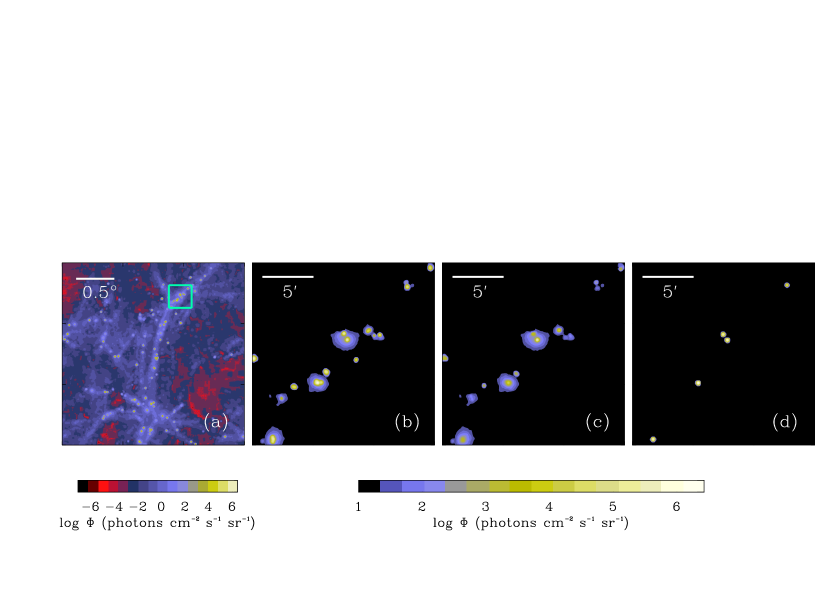
Figure 2.— Maps of Ly$\alpha$ surface brightness $\Phi$ for $z=0.15$ and $\Delta z=10^{-3}$ ($\Delta\lambda=1.2$ Å). Panel (a) assumes an angular resolution of $\sim 29\arcsec$; the rest show the region outlined in green with $7.2\arcsec$ resolution (or $\sim 13\,h^{-1}\mbox{ kpc}$). Except for panel (a), we exclude pixels with $\Phi<10\mbox{ photons cm${}^{-2}$ s${}^{-1}$ sr${}^{-1}$}$. (a), (b): Fiducial model. (c): $\varepsilon_{\alpha}=0$ for self-shielded gas. (d): Estimated Ly$\alpha$ emission from star formation in the slice (such emission was not included in the other panels).

Ly$\alpha$ emission occurs over a wide range of physical scales: generally, emitting regions have a central, high surface brightness ($\Phi\gtrsim 10^{3}\mbox{ photons cm${}^{-2}$ s${}^{-1}$ sr${}^{-1}$}$) core of size $\sim 30$–$50h^{-1}\mbox{ kpc}$ surrounded by an irregular, low surface brightness “corona” that can extend to scales $\gtrsim 10^{2}\mbox{ kpc}$. Thus, the Ly$\alpha$ emission is much more extended than the galaxies, indicating that this view of the cosmic web traces truly intergalactic gas.

Figure 3 shows histograms of the pixel flux probability distribution function (PDF) ${\rm d}P/{\rm d}\log\Phi$. The solid curve in each panel shows our fiducial model (using $\varepsilon_{\alpha}^{\rm coll}$ for self-shielded gas). Figure 3a shows the PDF to very small $\Phi$; we see a broad peak centered at $\Phi\sim 10^{-3}\mbox{ photons cm${}^{-2}$ s${}^{-1}$ sr${}^{-1}$}$ and a tail extending to much higher surface brightness. As described in Paper I, the location of the peak is determined simply by ionization equilibrium in the mean-density IGM and can be estimated analytically (Gould & Weinberg, 1996). Note that the PDF depends strongly on $\Delta\theta$, because the emitting regions have structure on small scales.

Figure 3.— The pixel surface brightness PDF in maps with $z=0.15$ (unless otherwise specified), $\Delta z=10^{-3}$ ($\Delta\lambda=1.2$ Å), and $13\,h^{-1}\mbox{ kpc}$ resolution. In all panels, the solid curve shows our fiducial model. (a): $\varepsilon_{\alpha}=0$ for self-shielded gas (dashed curve) and no self-shielding cut (dotted curve). (b): $z=0.07,\,0.15,\,0.3$, and $0.45$ (dotted, solid, long-dashed, and short-dashed curves, respectively). Also shown is the Ly$\alpha$ emission from star-forming gas (dot-dashed curve) at $z=0.15$. (c): $\varepsilon_{\alpha}=0$ for self-shielded gas, with $n_{\rm ss}=10^{-4},\,10^{-3}$, and $10^{-2}\mbox{ cm${}^{-3}$}$ (dotted, short-dashed, and long-dashed curves, respectively).

Figure 3b shows that the PDF evolves very little from $z=0.07$ to $z=0.45$. The fraction of bright pixels increases slowly with redshift because both the density and temperature of the IGM increase with redshift.

3.1. Ly$\alpha$ Photons From Star Formation

Figure 2d shows the Ly$\alpha$ emission from star formation. While all star-forming regions are surrounded by intergalactic Ly$\alpha$ emission, the converse is not true. We do find that Ly$\alpha$ emission nearly always surrounds star particles, but often these are dwarf galaxies or lack ongoing star formation. The exceptions are galaxies inside hot clusters, which do not always host Ly$\alpha$ emission. Note that Ly$\alpha$ emission produced through star formation is much more compact than the coronae (partly because we assume that all the ionizing photons are absorbed locally). Figure 3b compares the mechanisms in a more quantitative form. The emission from star-forming gas in the simulation (dot-dashed curve) dominates the brightest pixels but is unimportant for $\Phi\lesssim 10^{5}\mbox{ photons cm${}^{-2}$ s${}^{-1}$ sr${}^{-1}$}$. If a large fraction of the ionizing photons escape their host galaxy, the number of pixels affected by local star-formation will increase, but their mean brightness will also decrease. This could be particularly important near active galactic nuclei (AGN), which have large ionizing fluxes and large escape fractions. AGN could “light up” large volumes around their host galaxies in Ly$\alpha$ emission (Haiman & Rees, 2001). We note that the SFR, and hence Ly$\alpha$ emission from star-forming gas, increases with redshift (Hernquist & Springel, 2003).

3.2. Self-Shielded Gas

The largest uncertainty in our calculation is probably the treatment of self-shielded gas. One problem is identifying which particles are shielded from the ionizing background; we find, however, that our results do not change significantly in the range $10^{-4}\mbox{ cm${}^{-3}$}<n_{\rm ss}<10^{-2}\mbox{ cm${}^{-3}$}$, because most gas of these densities has $T\approx 10^{4.1}\mbox{ K}$, where $\varepsilon_{\alpha}^{\rm pi}\approx\varepsilon_{\alpha}^{\rm coll}$ (see Fig. 1). A more important concern is that we may have overestimated the temperature of self-shielded particles because the simulation erroneously allows the ionizing background to heat such particles and underestimates the cooling rates in optically thick regions. Radiative transfer calculations with CLOUDY suggest that the simulation may have overestimated the temperature of particles with $n_{\rm H}\sim 10^{-3}\mbox{ cm${}^{-3}$}$ by $\gtrsim 25\%$, which can be significant given the steep dependence seen in Figure 1. The error increases as the gas density and metallicity increase. In a worst case scenario, all self-shielded gas would have $T<10^{4.1}\mbox{ K}$, producing essentially no emission. In Figure 2c, we approximate this case by setting $\varepsilon_{\alpha}=0$ for all self-shielded gas. Comparing to the fiducial model, we find that the core brightness declines dramatically, but the extended coronae are unaffected. We conclude that the large-scale emission is due to optically thin gas while the brightest regions consist of gas at or near to the self-shielding threshold. The resulting PDF is shown as the short-dashed curve in Figure 3a; it essentially eliminates the bright tail of the distribution. Figure 3c shows that our results do depend on $n_{\rm ss}$ if self-shielded gas has $\varepsilon_{\alpha}=0$. The PDF changes little for $10^{-4}\mbox{ cm${}^{-3}$}<n_{\rm ss}<10^{-3}\mbox{ cm${}^{-3}$}$, because such gas has relatively low density and hence small emissivity. However, it approaches the fiducial model if we set $n_{\rm ss}=10^{-2}\mbox{ cm${}^{-3}$}$, because gas with $n_{\rm H}\gtrsim 10^{-2}\mbox{ cm${}^{-3}$}$ has $T\approx 10^{4.0}\mbox{ K}$ in the simulation and hence a small $\varepsilon_{\alpha}^{\rm coll}$.

On the other hand, the simulation also neglects local ionizing sources. We have already seen that most self-shielded particles reside near galaxies; we would therefore expect the radiation field around these particles to exceed the background. In this case the emissivity is limited by the ionizing flux reaching the gas. We have estimated the number of ionizing photons from young stars in §3.1, although we did not attempt to model the spatial distribution of the resulting emission. In addition, dense gas may no longer be self-shielded, so the diffuse background will also contribute to the Ly$\alpha$ emission. We estimate this extra component by assuming that no particles are self-shielded (dotted curve in Figure 3a). The number of bright pixels increases because $\varepsilon_{\alpha}^{\rm pi}\gg\varepsilon_{\alpha}^{\rm coll}$ for $T<10^{4.1}\mbox{ K}$. In either case, the net effect of local ionizing sources is to increase the Ly$\alpha$ emission.

4. Discussion

We study Ly$\alpha$ emission from gas in the IGM using a high-resolution cosmological simulation. We find that galaxies are typically surrounded by “coronae” of Ly$\alpha$ emission with bright, central cores (of diameter $\lesssim 40\,h^{-1}\mbox{ kpc}$) surrounded by much larger ($\gtrsim 10^{2}\,h^{-1}\mbox{ kpc}$) regions with surface brightness near the background. While the number of Ly$\alpha$ photons due to star formation in the host galaxies can exceed that emitted by the surrounding gas, the spatial extent of the star formation is typically much smaller. High angular-resolution observations (probing physical scales $\lesssim 15\,h^{-1}\mbox{ kpc}$) should be able to separate the two components. Detection of the bright cores is feasible with existing technology, although the wide-field ultraviolet spectrographs most useful for these studies have not yet been built. The Galaxy Evolution Explorer (GALEX), with a large field of view but relatively low spectral resolution ($\sim 10$ Å), may detect the brightest cores. Furthermore, the strong correlation between Ly$\alpha$ emission and galaxies may enable a statistical detection of the signal in deep exposures. A project underway to construct a balloon-borne wide-field UV spectrograph will have a limiting sensitivity $\Phi\sim 500\mbox{ photons cm${}^{-2}$ s${}^{-1}$ sr${}^{-1}$}$ in a single night’s observation (D. Schiminovich, private communication).

We emphasize that the emission from self-shielded gas is uncertain, because the simulation does not include all of the relevant physics. We have considered a range of models bracketing these uncertainties (see §3.2): in our fiducial model, dense, cool gas produces Ly$\alpha$ photons only through collisional processes, but we also consider cases in which it has zero emissivity or in which we allow photoionization. The choice has little effect on the large-scale, low surface brightness emission, which comes primarily from optically thin gas, but it does strongly affect the luminous cores., where most of the gas is shielded from the ionizing background.

We have also neglected dust, which can efficiently destroy Ly$\alpha$ photons. Because the emitting region is often considerably larger than the associated galaxy, much of the emitting gas may be relatively pristine. In the simulation, we find that the majority of particles with large Ly$\alpha$ emissivity contain no metals (or dust), though note that the simulation does not include mixing between simulation particles. At higher redshifts, several large-scale Ly$\alpha$-emitting “blobs” have already been observed (e.g., Steidel et al. 2000), limiting the amount of dust in these environments.

The structure and relatively large spatial size of Ly$\alpha$ emitters, together with their locations, suggest that they are “cooling flows” of gas onto halos. Detailed, high resolution Ly$\alpha$ observations therefore offer a means to study the accretion and cooling of gas onto galaxies. Galactic winds will also affect the distribution of Ly$\alpha$ emission. However, we find that the winds in our simulations have only minor effects on the statistics of Ly$\alpha$ emitters.

On larger scales, the Ly$\alpha$ emitters are distributed along sheets and filaments. Because these objects are numerous (with a space density $\sim 0.1h^{3}$ Mpc^-3), Ly$\alpha$ line observations offer a new and powerful way to map the cosmic web. Figure 2 shows that such observations do not require high resolution; wide-field observations could efficiently locate (in three dimensions) a large number of Ly$\alpha$ emitters. In contrast to galaxy surveys, this approach reveals the location of baryons outside of galaxies. Because Ly$\alpha$ emission traces the cool gas accreting onto galaxies, it also selects a different population of dark matter halos, including many with few (or even no) associated stars. Follow-up observations at high resolution would allow us to compare Ly$\alpha$ emitters to galaxy surveys and learn how galaxies accrete gas at the present day.

References

- Brown et al. (2000) Brown, T. M., et al. 2000, AJ, 120, 1153
- de Lapparent et al. (1986) de Lapparent, V., Geller, M. J., & Huchra, J. P. 1986, ApJ, 302, L1
- Fardal et al. (2001) Fardal, M. A., et al. 2001, ApJ, 562, 605
- Ferland (2003) Ferland, G. J. 2003, Hazy, A Brief Introduction to Cloudy 96.00 (http://www.nublado.org/)
- Furlanetto et al. (2003) Furlanetto, S. R., Schaye, J., Springel, V., & Hernquist, L. 2003, ApJ, submitted (astro-ph/0309736) [F03]
- Gould & Weinberg (1996) Gould, A., & Weinberg, D. H. 1996, ApJ, 468, 462
- Haardt & Madau (2001) Haardt, F., & Madau, P. 2001, in Clusters of Galaxies and the High Redshift Universe Observed in X-rays, ed. D. M. Neumann & J. T. T. Van (21st Moriond Astrophysics Meeting, Les Arc, France)
- Haiman & Rees (2001) Haiman, Z. & Rees, M. J. 2001, ApJ, 556, 87
- Haiman et al. (2000) Haiman, Z., Spaans, M., & Quataert, E. 2000, ApJ, 537, L5
- Hernquist & Springel (2003) Hernquist, L., & Springel, V. 2003, MNRAS, 341, 1253
- Hogan & Weymann (1987) Hogan, C. J., & Weymann, R. J. 1987, MNRAS, 225, 1P
- Katz et al. (1996) Katz, N., Weinberg, D. H., & Hernquist, L. 1996, ApJS, 105, 19
- Kunth et al. (2003) Kunth, D., et al. 2003, ApJ, in press (astro-ph/0307555)
- Leitherer et al. (1999) Leitherer, C., et al. 1999, ApJS, 123, 3
- Möller & Fynbo (2001) Möller, P., & Fynbo, J. U. 2001, A&A, 372, L57
- Osterbrock (1989) Osterbrock, D. E. 1989, Astrophysics of Gaseous Nebulae and Active Galactic Nuclei (Mill Valley, CA: Univ. Sci.)
- Rauch (1998) Rauch, M. 1998, ARA&A, 36, 267
- Schaye (2001) Schaye, J. 2001, ApJ, 562, L95
- Spergel et al. (2003) Spergel, D. N., et al. 2003, ApJS, 148, 175
- Springel & Hernquist (2003a) Springel, V., & Hernquist, L. 2003a, MNRAS, 339, 289
- Springel & Hernquist (2003b) —. 2003b, MNRAS, 339, 312
- Steidel et al. (2000) Steidel, C. C.et al. 2000, ApJ, 532, 170