Inflationary potentials yielding constant scalar perturbation spectral indices

Abstract

We explore the types of slow-roll inflationary potentials that result in scalar perturbations with a constant spectral index, i.e., perturbations that may be described by a single power-law spectrum over all observable scales. We devote particular attention to the type of potentials that result in the Harrison–Zel’dovich spectrum.

I Introduction

Inflation, a cornerstone of the modern framework for understanding the early universe guth81 ; lrreview , predicts the initial conditions for the formation of structure and the cosmic microwave background (CMB) anisotropies. During inflation, the primordial scalar (density) and tensor (gravitational wave) perturbations generated by quantum fluctuations are redshifted beyond the Hubble radius, becoming frozen as perturbations in the background metric muk81 ; hawking82 ; starobinsky82 ; guth82 ; bardeen83 . However, even when there is only one scalar field — the inflaton — the number of inflation models proposed in the literature is large lrreview . Determination of the properties of the scalar perturbations and tensor perturbations from CMB and large-scale structure observations allows one to constrain the space of possible inflation models dodelson97 ; kinney98a ; probes ; wmapinf ; barger ; kkmr ; liddleleach .

It is often adequate to characterize inflationary perturbations in terms of four quantities: the scalar and tensor power spectra, $\mathcal{P}_{\mathcal{R}}$ and $\mathcal{P}_{g}$, and the scalar and tensor spectral indices $n$ and $n_{T}$. In this paper we focus on the scalar spectral index which, unless explicitly indicated otherwise, we refer to simply as the ‘spectral index’. Successful inflation models predict $n$ close to $1$ (the so-called Harrison–Zel’dovich spectrum), and $n$ typically has a small scale dependence. The best data available to date, combining the Wilkinson Microwave Anisotropy Probe wmap and Sloan Digital Sky Survey SDSS data sets, indicate that the evidence for anything other than a scale-invariant spectra is marginal at best, with no evidence for significant running of the scalar spectral index tegmarksloan . Moreover, one of us has recently argued that when information criteria are used to carry out cosmological model selection based on the current data sets available, then the best present description of cosmological data uses a scale-invariant ($n=1$) spectrum liddleparameters . It therefore makes sense to be considering the inflationary potentials associated with that spectrum.

It is known that inflaton potentials $V(\phi)=\exp(-\alpha\phi)$ for constant $\alpha^{2}<2$ lead to perturbation spectra that are exact power laws, i.e. $n$ is a constant lucchin . However, there has not yet been a systematic analysis of the types of inflaton potentials that yield constant $n$. Here we take a first step in that direction, classifying those potentials within the framework of the slow-roll approximation SRref .

In the next section the basic results employed to calculate the properties of the perturbation spectrum using the slow-roll parameterization of the inflaton potential are reviewed. In Sec. III two exact differential equations connecting the potential and the field to the slow-roll parameters are derived and the general method used to calculate all the relevant cosmological quantities is outlined. In Sec. IV this method is applied to the determination of the inflationary potential yielding a $k$-independent density spectral index: both the Harrison–Zel’dovich $(n=1)$ and the general $(n=1-2n_{0}^{2})$ case are considered to lowest order and to next order in the slow-roll parameter approximation. In Sec. V the flow of $\epsilon$ is examined to understand the number of solutions that arise. The conclusions are contained in Sec. VI.

II Review of Basic Concepts

II.1 Inflationary Dynamics and Slow Roll Parameters

The dynamics of the standard Friedmann–Robertson–Walker (FRW) universe driven by the potential energy of a single scalar field – the inflaton $\phi$ – are usually expressed by the Friedmann equation for flat spatial sections and by the energy conservation equation:

$$H^{2} = \frac{8\pi}{3M_{{\rm p}}^{2}}\left[\frac{1}{2}\dot{\phi}^{2}+V(\phi)\right],$$ (2)

$$\ddot{\phi}+3H\dot{\phi}+V^{\prime}(\phi)=0,$$

where $V(\phi)$ is the inflaton potential, $M_{{\rm p}}=G^{-1/2}$ the Planck mass and $H=\dot{a}/a$ the Hubble expansion parameter. Once $V(\phi)$ is specified, the field dynamics are determined by solving the coupled equations (2) and (2). Often it is simplest to do this using the Hamilton–Jacobi approach HJref in which $H(\phi)$ is considered the fundamental quantity to be specified. Equations (2) and (2) then become two first-order equations:

$$H^{\prime}(\phi)^{2}-12\pi H^{2}(\phi)/M_{{\rm p}}^{2} = -32\pi^{2}V(\phi)/M_{{\rm p}}^{4}\,;$$ (3)

$$\dot{\phi} = -M_{{\rm p}}^{2}H^{\prime}(\phi)/4\pi\,,$$ (4)

where ${}^{\prime}\equiv d/d\phi$. Whichever the method, once the dynamics of the inflaton field is known, $a(t)$ is obtained by integrating Eq. (2). Without any loss of generality we assume that $\dot{\phi}>0$ during inflation. Here we use the Hubble slow-roll parameters $\epsilon$, $\eta$ and $\xi^{2}$ as defined in Ref. LPB

$$\epsilon(\phi) \equiv \frac{3\dot{\phi}^{2}}{2}\left[V(\phi)+\frac{\dot{\phi}^{2}}{2}\right]^{-1}=\frac{M_{{\rm p}}^{2}}{4\pi}{\left[\frac{H^{\prime}(\phi)}{H(\phi)}\right]}^{2},$$ (5)

$$\eta(\phi) \equiv -\frac{\ddot{\phi}}{H\dot{\phi}}=\frac{M_{{\rm p}}^{2}}{4\pi}\frac{H^{\prime\prime}(\phi)}{H(\phi)},$$ (6)

$$\xi^{2}(\phi) \equiv \frac{M_{{\rm p}}^{4}}{16\pi^{2}}\frac{H^{\prime}(\phi)H^{\prime\prime\prime}(\phi)}{H^{2}(\phi)}.$$ (7)

The parameters $\eta$ and $\xi^{2}$ are the first terms in an infinite hierarchy of slow-roll parameters, whose $l$-th member is defined by

$$\lambda_{H}^{l}(\phi)\equiv\left(\frac{M_{{\rm p}}^{2}}{4\pi}\right)^{l}\frac{(H^{\prime})^{l-1}}{H^{l}}\frac{d^{(l+1)}H(\phi)}{d\phi^{(l+1)}}.$$ (8)

During slow-roll $\{\epsilon,\lambda_{H}^{l}\}\ll 1$, and inflation ends when $\epsilon=1$. The potential and its derivatives can be expressed as exact functions of these slow-roll parameters: up to second order in derivatives of $V$ one has

$$V(\phi) = \frac{M_{{\rm p}}^{2}}{8\pi}H^{2}(3-\epsilon),$$ (9)

$$\frac{dV(\phi)}{d\phi} = -\frac{M_{{\rm p}}}{2\sqrt{\pi}}H^{2}\sqrt{\epsilon}(3-\eta),$$ (10)

$$\frac{d^{2}V(\phi)}{d\phi^{2}} = H^{2}\left[3\epsilon+3\eta-(\eta^{2}+\xi^{2})\right].$$ (11)

II.2 A Hierarchy of Approximation Orders

As mentioned in the introduction, the observable quantities of interest are the power spectrum $\mathcal{P}_{\mathcal{R}}$ of the curvature perturbation $\mathcal{R}$ on comoving hypersurfaces and the spectrum of gravity waves $\mathcal{P}_{g}$. These define $n(k)$ and $n_{T}(k)$ through

$$n(k)-1 \equiv \frac{d\ln\mathcal{P}_{\mathcal{R}}(k)}{d\ln k},$$ (12)

$$n_{T}(k) \equiv \frac{d\ln\mathcal{P}_{g}(k)}{d\ln k}.$$ (13)

As discussed in Ref. Lidsey:1995np ; Stewart:1993bc , the expressions for these quantities differ depending on the approximation order assumed in the slow-roll expansion. The approximation order is defined in general by considering how many terms in a slow-roll parameter expansion of a generic expression are retained, lowest-order approximation corresponding to retaining only the lowest-order term and next-order approximation corresponding to retaining terms up to the next-to-lowest order term.

For the perturbation power spectra and spectral indices, the lowest-order term is linear in the slow-roll parameters. To order $l_{0}$, these expressions will contain the set of slow-roll parameters $\{\epsilon,\lambda_{H}^{l}\}$ with $l=(1,2,..l_{0})$ where $\lambda_{H}^{l}$ is a term of order $l$. At next-order ($l_{0}=2$), the expressions will contain the parameters $\{\epsilon,\eta,\xi^{2}\equiv\lambda_{H}^{2}\}$ as well as all second-order combinations thereof (namely $\epsilon^{2},\eta^{2}$ and $\eta\epsilon$). Hence, for order consistency, whenever an exact and an approximate expression are combined (as shall often be the case below) the result is accurate only to the order of the approximate expression, and the result must be expanded in a power series of slow-roll parameters up to and including terms of an overall degree consistent with the level of approximation assumed.

Recalling Lidsey et al. Lidsey:1995np , it is then possible to think of an infinite hierarchy of expressions for the perturbation spectra and for the spectral indices. It is unfortunate that, due to the complexity of the problem, only the first two approximation orders are currently available in general: indeed, at next-to-lowest order,

$$\mathcal{P}_{\mathcal{R}}^{1/2}(k) \simeq 2\left[1-\{(2C+1)\epsilon-C\eta\}\right]\left.\frac{H^{2}}{M_{{\rm p}}^{2}|H^{\prime}|}\right|_{k=aH}$$ (14)

$$\mathcal{P}_{g}^{1/2}(k) \simeq \frac{4}{\sqrt{\pi}}\left[1-\{(C+1)\epsilon\}\right]\left.\frac{H}{M_{{\rm p}}}\right|_{k=aH},$$ (15)

$$n(k)-1 \simeq -4\epsilon+2\eta-\{8(C+1)\epsilon^{2}$$ (16)

$$-(6+10C)\epsilon\eta+2C\xi^{2}\},$$

$$n_{T}(k) \simeq -2\epsilon-\{2\epsilon^{2}(3+2C)-4(1+C)\epsilon\eta\},$$ (17)

where $C\simeq-0.73$ Lidsey:1995np ; Stewart:1993bc . As in Ref. Lidsey:1995np , the symbol “$\simeq$” is used to indicate that the results are accurate up to the order of approximation assumed. The lowest-order results are obtained by setting all the terms in curly brackets to zero.

III The Parametrization Method

We now focus on the case of constant $n(k)$. To any order $l_{0}$ in the slow-roll approximation, imposing $k$-independence of $n(k)$ endows the problem with the additional set of $(l_{0}-1)$ relations

$$\frac{d^{i}n(k)}{d(\ln k)^{i}}=0,\qquad i=1,\ldots,(l_{0}-1).$$ (18)

Therefore, since there are $l_{0}+1$ slow-roll parameters at this order, the conditions (18) together with the constancy of $n(k)$ mean that only one of those is independent: throughout the rest of this paper we take it to be $\epsilon$. As we show in this section, it is then possible to determine $\phi(\epsilon)$ and $V(\phi)$ to this order.

The method is the following. First we derive two exact differential equations for $\phi$ and $V$ which, as we shall see below, only contain the slow-roll parameters $\eta$ and $\epsilon$. Then, at a given order $l_{0}$, we impose the conditions given in Eq. (18) which yield $\eta(\epsilon)$. As a result the two differential equations can be integrated to obtain $V(\epsilon)$ and $\phi(\epsilon)$ correct to order $l_{0}$. Finally, provided $\phi(\epsilon)$ can be inverted, we can obtain $V(\phi)$. This will be done in the next section where we also solve for all the dynamics of the problem, namely $H(\phi)$, $a(t)$ and $\phi(t)$.

From Eq.(5) it is straightforward to obtain

$$\frac{d\epsilon}{d\phi}=\frac{2M_{{\rm p}}^{2}}{4\pi}\left[\frac{H^{\prime}H^{\prime\prime}}{H^{2}}-{\left(\frac{H^{\prime}}{H}\right)}^{3}\right],$$ (19)

which, together with the definitions of $\epsilon$ and $\eta$, yields the exact differential equation

$$\frac{d\epsilon}{d\phi}=\frac{4\sqrt{\pi}}{M_{{\rm p}}}\sqrt{\epsilon}(\epsilon-\eta)\,.$$ (20)

Once $\eta(\epsilon)$ is specified, integration of this equation yields $\phi(\epsilon)$.

Also, Eqs. (10) and (20) give

$$\frac{dV}{d\epsilon}=\frac{dV}{d\phi}\frac{d\phi}{d\epsilon}=-\frac{M_{{\rm p}}^{2}H^{2}}{8\pi}\left[\frac{3-\eta}{\epsilon-\eta}\right],$$ (21)

which, divided by Eq. (9), produces the following exact differential equation, useful because it is independent of the Hubble parameter:

$$\frac{1}{V}\frac{dV}{d\epsilon}=\frac{3-\eta}{(\eta-\epsilon)(3-\epsilon)}=\frac{1}{\epsilon-3}+\frac{1}{\eta-\epsilon}.$$ (22)

Given $\eta(\epsilon)$, Eq. (22) can be integrated to give

$$V(\epsilon)=V_{0}|3-\epsilon|\exp\left[\int\frac{d\epsilon}{\eta(\epsilon)-\epsilon}\right],$$ (23)

where $V_{0}$ is the integration constant which can be obtained from the observed perturbation amplitude. Finally from Eq. (9) the following expression for $H$ can be obtained

$$H^{2}(\epsilon)=\frac{8\pi V_{0}}{M_{{\rm p}}^{2}}\exp\left[\int\frac{d\epsilon}{\eta(\epsilon)-\epsilon}\right].$$ (24)

As noted in the previous section, once the integrations in Eqs. (23) and (24) have been carried out, order consistency requires that the resulting expressions are expanded in powers of $\epsilon$ and only terms up to and including order $l_{0}$ are kept.

Once the expressions for $V(\epsilon)$ and $\phi(\epsilon)$ have been computed, it is then possible to determine all the other relevant cosmological quantities. Eq. (24) together with the expression for $\epsilon(\phi)$ gives $H(\phi)$ to the given order $l_{0}$. This, together with the equation obtained for $V(\phi)$ then enables $\phi(t)$ to be calculated using Eq. (2). Once this step is carried out, the time evolution of the Hubble parameter can be derived – either using Eq. (2) or the solution of Eq. (24) – and its integration then yields the dynamics of the scale factor $a(t)$.

Before turning to the specific cases of constant spectral index, it is worth commenting on the apparently singular case of $\eta=\epsilon$. This is nothing other than the usual exact power-law inflation model and is perfectly regular. From Eq. (20), we see that in this case the solution is $\epsilon=\epsilon_{0}$, a constant independent of $\phi$. Substituting this value into Eqs. (5) and (9) we obtain

$$H = {\sqrt{8\pi V_{0}}\over M_{{\rm p}}}\exp\left[-{2\sqrt{\pi\epsilon_{0}}\phi\over M_{{\rm p}}}\right]$$ (25)

$$V = V_{0}(3-\epsilon_{0})\exp\left[-{4\sqrt{\pi\epsilon_{0}}\phi\over M_{{\rm p}}}\right].$$ (26)

Substituting this into the Friedmann equation, Eq. (2), we obtain $\phi(t)$ through

$$\sqrt{8\pi V_{0}}{\epsilon_{0}t\over M_{{\rm p}}}=\exp\left[{2\sqrt{\pi\epsilon_{0}}\phi\over M_{{\rm p}}}\right]\,.$$ (27)

Hence in Eq. (25) we find $a(t)\sim t^{p}$ where $p=1/\epsilon_{0}$, the usual power-law inflation result.

Finally, we note that it is also possible to address the present problem using the definitions of the slow-roll parameters in the expression for the spectral index to obtain a differential equation for $H(\phi)$ beato . While at lowest-order this approach yields results which are equivalent to the ones derived in the next section, the differential equation arising at next-order does not seem to allow an analytical solution and in that case the parametrization method outlined above proves to be preferable.

IV Applications

In this section the method outlined above is applied to the determination of the inflationary potentials which yield a $k$-independent spectral index. Two cases will be considered: the Harrison–Zel’dovich power spectrum, and the case of a $k$-independent spectral index not equal to unity. For each case, both lowest-order and next-order approximation results will be derived.

IV.1 The Harrison–Zel’dovich Case

IV.1.1 Lowest-order approximation

Imposing $n(k)=1$ in the lowest-order expression for the spectral index, Eq. (16), yields

$$\eta(\epsilon)\simeq 2\epsilon.$$ (28)

Thus Eqs. (20) and (23) become

$$\frac{d\epsilon}{d\phi} \simeq -\frac{4\sqrt{\pi}}{M_{{\rm p}}}\epsilon^{3/2},$$ (29)

$$\frac{d\ln V}{d\epsilon} \simeq \frac{1}{\epsilon-3}+\frac{1}{\epsilon},$$ (30)

which can be integrated immediately, giving

$$\phi(\epsilon) \simeq \frac{M_{{\rm p}}}{2\sqrt{\pi\epsilon}},$$ (31)

$$V(\epsilon) \simeq V_{0}(3-\epsilon)\epsilon\simeq V_{0}3\epsilon,$$ (32)

and hence

$$V(\phi)\simeq V_{0}\frac{3M_{{\rm p}}^{2}}{4\pi\phi^{2}}.$$ (33)

Eq. (24) then yields

$$H^{2}(\phi)\simeq\frac{8\pi V_{0}}{M_{{\rm p}}^{2}}\epsilon\simeq\frac{2V_{0}}{\phi^{2}}\,,$$ (34)

and the constant $V_{0}$ can be read off from the lowest-order version of Eq. (14) as

$$V_{0}\simeq\frac{M_{{\rm p}}^{4}}{8}\,{\cal P}_{\cal R}\,.$$ (35)

This, together with the expression for $V^{\prime}(\phi)$, can then be used in the Friedmann equation which becomes

$$\phi^{2}\dot{\phi}\simeq\frac{\sqrt{2V_{0}}M_{{\rm p}}^{2}}{4\pi},$$ (36)

so that

$$\phi(t)\simeq\phi_{0}\ (t/t_{0})^{1/3},$$ (37)

where $\phi_{0}^{3}t_{0}^{-1}=3\sqrt{2V_{0}}M_{{\rm p}}^{2}/4\pi$. Eq. (31) can then be used to compute the dynamics of the slow-roll parameter

$$\epsilon(t)\simeq\frac{M_{{\rm p}}^{2}}{4\pi\phi_{0}^{2}}\left(t/t_{0}\right)^{-2/3}.$$ (38)

Finally, the time evolution of the Hubble parameter and of the scale factor are given by:

$$H(t) \simeq H(t_{0})\left(t/t_{0}\right)^{-1/3},$$

$$\frac{a(t)}{a(t_{0})} \simeq \exp\left\{\frac{\sqrt{8V_{0}}}{3\phi_{0}t_{0}^{-1}}\left[\left(\frac{t}{t_{0}}\right)^{2/3}-1\right]\right\}.$$ (39)

Let us now recall the work of Barrow and Liddle on intermediate inflation Barrow:1993zq . Though the present work differs in spirit from that paper (which starts by postulating a specific dynamics and then goes on to derive the corresponding potential), the two approaches share a common point, as we now outline. In Ref. Barrow:1993zq the scale factor is assumed to take the form

$$a(t)=\exp\left(At^{f}\right),$$ (40)

with $0<f<1$, $A>0=$ constants. The authors then prove that this is an exact solution of the ‘intermediate’ inflation potential

$$V(\phi)=\frac{8A^{2}}{(\beta+4)^{2}}\left[\frac{(2A\beta)^{1/2}}{\phi}\right]^{\beta}\left[6-\frac{\beta^{2}}{\phi^{2}}\right],$$ (41)

where $\beta=4(f^{-1}-1)$, and that it is also a solution in the slow-roll approximation for the potential

$$V(\phi)=\frac{48A^{2}}{(\beta+4)^{2}}\left[\frac{(2A\beta)^{1/2}}{\phi}\right]^{\beta}.$$ (42)

To see how the present results relate to the ones reported in Ref. Barrow:1993zq , we first quote the expressions for the slow-roll parameters obtained in the intermediate inflation case:

$$\epsilon=\frac{\beta^{2}}{2\phi^{2}}\,;\quad\eta=\left(1+\frac{\beta}{2}\right)\frac{\beta}{\phi^{2}}\,.$$ (43)

Exploiting Eq. (43), the equation for the exact intermediate inflation potential can be recast in the form

$$V(\phi)=\frac{16A^{2}}{(\beta+4)^{2}}\left[\frac{(2A\beta)^{1/2}}{\phi}\right]^{\beta}[3-\epsilon(\phi)].$$ (44)

Now, we can think of this expression as a function of the slow-roll parameter $\epsilon$ instead of the field $\phi$. In this perspective, neglecting the $\epsilon$ in the $(3-\epsilon)$ factor is the same as saying that lowest-order slow-roll approximation is assumed and that by order consistency one should retain only the lowest-order term arising from $\phi^{-\beta}(\epsilon)$. In other words, the $\epsilon$ appearing in the $(3-\epsilon)$ factor will generate terms of higher order, all of which can be consistently neglected in a lowest-order calculation.

Note furthermore that imposing the $n(k)=1$ condition in the form consistent with the lowest-order approximation (that is, $\eta=2\epsilon$) and using Eq. (43) yields $\beta=2$ and $f=2/3$. This is consistent with the previous calculation, since inserting this value of $\beta$ into Eq. (42) produces an expression for the inflaton potential analogous to Eq. (33)

$$V(\phi)\sim\frac{3}{\phi^{2}},$$ (45)

thus showing that the present analysis and the one carried out by Barrow and Liddle in Ref. Barrow:1993zq agree on the lowest-order potential able to produce a Harrison–Zel’dovich density power spectrum.

IV.1.2 Next-order approximation

As discussed at the beginning of Sec. III, the two conditions given in Eq. (18) must now be imposed in order to determine $\eta(\epsilon)$. The first condition is simply obtained from Eq. (16): imposing $n(k)=1$ at next-order gives

$$4\epsilon-2\eta+8(C+1)\epsilon^{2}-(6+10C)\epsilon\eta+2C\xi^{2}\simeq 0.$$ (46)

The second condition, $dn/d\ln k=0$, yields Lidsey:1995np

$$-2\xi^{2}-8\epsilon^{2}+10\epsilon\eta\simeq 0.$$ (47)

These expressions then allow us to solve for $\xi^{2}$ and $\eta$ as functions of $\epsilon$, giving

$$\eta(\epsilon) \simeq \frac{2\epsilon+4\epsilon^{2}}{3\epsilon+1}\simeq 2\epsilon-2\epsilon^{2},$$

$$\xi^{2}(\epsilon) \simeq \frac{6\epsilon^{2}+8\epsilon^{3}}{3\epsilon+1}\simeq 6\epsilon^{2}.$$ (48)

Eqs. (20) and (23) become

$$\frac{d\epsilon}{d\phi} \simeq -\frac{4\sqrt{\pi}}{M_{{\rm p}}}\sqrt{\epsilon}\;\frac{\epsilon(\epsilon+1)}{3\epsilon+1},\qquad$$ (49)

$$\frac{d\ln V}{d\epsilon} \simeq \frac{1}{\epsilon-3}+\frac{3\epsilon+1}{\epsilon(\epsilon+1)}.$$ (50)

These can be integrated exactly to yield

$$\phi(\epsilon) \simeq \frac{M_{{\rm p}}}{2\sqrt{\pi}}\left[\frac{1}{\sqrt{\epsilon}}-2\tan^{-1}(\sqrt{\epsilon})\right]$$ (51)

$$\simeq\frac{M_{{\rm p}}}{2\sqrt{\pi}}\left(\frac{1}{\sqrt{\epsilon}}-2\sqrt{\epsilon}\right),$$

$$V(\epsilon) \simeq V_{0}\epsilon(3-\epsilon)(1+\epsilon)^{2}\simeq V_{0}(3\epsilon+5\epsilon^{2}).$$ (52)

In this case it is neither straightforward nor very enlightening to obtain an explicit expression for the potential as a function of the field. Numerically, however, we can determine $V(\phi)$ from Eqs. (51) and (52). The result is plotted in Fig. 1 together with the lowest-order result.

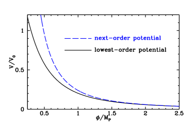
Figure 1: Potentials giving the Harrison–Zel’dovich density spectral index, computed to lowest-order approximation and to next-order approximation.

IV.2 General power-laws

Having determined the inflationary potential generating a Harrison–Zel’dovich spectrum, in this Section we consider the more general case for which

$$n(k)=1-2n_{0}^{2}\qquad\forall k.$$ (53)

We focus primarily on the $n_{0}^{2}>0$ case: the results for $n_{0}^{2}<0$ are obtained by analytic continuation, with some care being taken over the number of solutions available in that case.

IV.2.1 Lowest-order approximation

Inserting the lowest-order expression for $n(k)$, Eq. (16), into Eq. (53), gives

$$\eta(\epsilon)\simeq 2\epsilon-n_{0}^{2},$$ (54)

so that Eqs. (20) and (23) become

$$\frac{d\epsilon}{d\phi} \simeq \frac{4\sqrt{\pi}}{M_{{\rm p}}}\sqrt{\epsilon}(n_{0}^{2}-\epsilon),$$ (55)

$$\frac{d\ln V}{d\epsilon} \simeq \frac{1}{\epsilon-3}+\frac{1}{\epsilon-n_{0}^{2}}.$$ (56)

Let’s first consider the $n_{0}^{2}>0$ case. Depending on whether $\epsilon>n_{0}^{2}$ or $\epsilon<n_{0}^{2}$, integration of Eq. (55) above yields

$$\phi(\epsilon)\simeq\frac{M_{{\rm p}}}{2n_{0}\sqrt{\pi}}\left\{\begin{array}[]{cc}\coth^{-1}\left(\sqrt{\epsilon/{n_{0}^{2}}}\right)&\qquad(\epsilon>n_{0}^{2})\\ \tanh^{-1}\left(\sqrt{\epsilon/{n_{0}^{2}}}\right)&\qquad(\epsilon<n_{0}^{2})\\ \end{array}\right.$$ (57)

Similarly, integration of Eq. (56) gives

$$V(\epsilon)\simeq V_{0}(3-\epsilon)|\epsilon-n_{0}^{2}|\simeq\pm V_{0}[\epsilon(3+n_{0}^{2})-3n_{0}^{2}],$$ (58)

where upper (lower) sign refers to the $\epsilon>n_{0}^{2}$ $(\epsilon<n_{0}^{2})$ case. Combining these results produces

$$V(\phi)\simeq V_{0}n_{0}^{2}\left\{\begin{array}[]{cc}-3+(3+n_{0}^{2})\coth^{2}\left(\frac{\displaystyle{2n_{0}\sqrt{\pi}}}{\displaystyle{M_{{\rm p}}}}\phi\right)&(\epsilon>n_{0}^{2})\\ 3-(3+n_{0}^{2})\tanh^{2}\left(\frac{\displaystyle{2n_{0}\sqrt{\pi}}}{\displaystyle{M_{{\rm p}}}}\phi\right)&(\epsilon<n_{0}^{2})\\ \end{array}\right.$$ (59)

Examples of such potentials for $\epsilon>n_{0}^{2}$ are illustrated in Fig. 2.

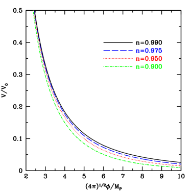
Figure 2: Four potentials computed to lowest order, yielding density perturbation spectral indices of 0.9, 0.95, 0.975, 0.99.

When $n_{0}^{2}<0$, the corresponding lowest-order results for $V(\epsilon)$ and $\phi(\epsilon)$ are given by

$$V(\epsilon)\simeq V_{0}\left[\epsilon(3+n_{0}^{2})-3n_{0}^{2}\right],$$ (60)

and

$$\phi(\epsilon)\simeq\frac{M_{{\rm p}}}{2\sqrt{\pi|n_{0}^{2}|}}\tan^{-1}\left(\sqrt{\frac{\epsilon}{|n_{0}^{2}|}}\right).$$ (61)

Inverting Eq. (61) we obtain

$$V(\phi)\simeq V_{0}|n_{0}^{2}|\left[(3+n_{0}^{2})\tan^{2}\left(\frac{2\phi\sqrt{\pi|n_{0}^{2}|}}{M_{{\rm p}}}\right)-3\right],$$ (62)

where now only one solution exists because $\epsilon-n_{0}^{2}>0$.

At this point it seems rather puzzling that there are two different solutions for the potential when $n_{0}^{2}>0$, and only one when $n_{0}^{2}<0$. In Sec. V it will be shown that the reason for this is related to the behavior that Eq. (55) exhibits as a function of the initial value of the slow-roll parameter, $\epsilon_{0}$.

IV.2.2 Next-order approximation

First it is necessary to express the slow-roll parameters $\eta$ and $\xi^{2}$ as functions of $\epsilon$ and $n_{0}^{2}$. At next-order the condition (53) gives

$$4\epsilon-2\eta+8(C+1)\epsilon^{2}-(6+10C)\epsilon\eta+2C\xi^{2}\simeq 2n_{0}^{2}.$$ (63)

On imposing the condition $dn(k)/d\ln k=0$ we find

$$\eta(\epsilon) \simeq \frac{2\epsilon+4\epsilon^{2}-n_{0}^{2}}{3\epsilon+1}$$

$$\simeq-n_{0}^{2}+(2+3n_{0}^{2})\epsilon-(2+9n_{0}^{2})\epsilon^{2},$$

$$\xi^{2}(\epsilon) \simeq \frac{6\epsilon^{2}+8\epsilon^{3}-5n_{0}^{2}\epsilon}{3\epsilon+1}$$

$$\simeq-5n_{0}^{2}\epsilon+(6+15n_{0}^{2})\epsilon^{2},$$

so that Eqs. (20) and (23) in this case take the form

$$\frac{d\phi}{d\epsilon} \simeq -\frac{M_{{\rm p}}}{4\sqrt{\pi}}\frac{1}{\sqrt{\epsilon}}\frac{3\epsilon+1}{\epsilon^{2}+\epsilon-n_{0}^{2}},$$ (66)

$$\frac{d\ln V}{d\epsilon} \simeq \frac{1}{\epsilon-3}+\frac{3\epsilon+1}{\epsilon^{2}+\epsilon-n_{0}^{2}}.$$ (67)

To solve these equations, let $a$ and $b$ be the two roots of $\epsilon^{2}+\epsilon-n_{0}^{2}=0$ so that

$$2a=-1-\delta\;,2b=-1+\delta\;\;\;{\rm with}\;\;\;\delta=\sqrt{1+4n_{0}^{2}}.$$ (68)

Furthermore we assume $0<n_{0}^{2}\ll 1$, so that $a\simeq-(1+n_{0}^{2})<0$ and $b\simeq n_{0}^{2}>0$. Using

$$\frac{3\epsilon+1}{\epsilon^{2}+\epsilon-n_{0}^{2}}=\frac{p_{+}}{\epsilon-a}+\frac{p_{-}}{\epsilon-b}\;\;\;{\rm with}\;\;\;p_{\pm}=\frac{(3\pm\delta^{-1})}{2}$$ (69)

one can integrate Eq. (66) to find, in the cases $\epsilon>b\simeq n_{0}^{2}$ and $\epsilon<b\simeq n_{0}^{2}$ respectively,

$$\phi(\epsilon)\simeq\frac{M_{{\rm p}}}{2\sqrt{\pi}}\left\{\begin{array}[]{c}-\frac{\displaystyle{p_{+}}}{\displaystyle{\sqrt{|a|}}}\tan^{-1}\sqrt{\frac{\displaystyle{\epsilon}}{\displaystyle{|a|}}}+\frac{\displaystyle{p_{-}}}{\displaystyle{\sqrt{b}}}\coth^{-1}\sqrt{\frac{\displaystyle{\epsilon}}{\displaystyle{b}}}\\ -\frac{\displaystyle{p_{+}}}{\displaystyle{\sqrt{|a|}}}\tan^{-1}\sqrt{\frac{\displaystyle{\epsilon}}{\displaystyle{|a|}}}+\frac{\displaystyle{p_{-}}}{\displaystyle{\sqrt{b}}}\tanh^{-1}\sqrt{\frac{\displaystyle{\epsilon}}{\displaystyle{b}}}\\ \end{array}\right.$$ (70)

Finally, integration of Eq. (67) yields

$$V(\epsilon)\simeq V_{0}(3-\epsilon)\left|\epsilon-a\right|^{p_{+}}\left|\epsilon-b\right|^{p_{-}}$$ (71)

As in Sec. IV.1.2 the potential and the field have been successfully parametrized with respect to $\epsilon$: they can be inverted numerically to find $V(\phi)$.

V The flow of $\epsilon$

As was pointed out in Sec. IV.2, it is interesting that more than one solution arises in the general power-law case. To further explore the reason for this, it is necessary to consider again the evolution of $\epsilon(\phi)$ given by Eq. (55), keeping in mind that without loss of generality $\dot{\phi}>0$ is assumed.

V.1 The $n_{0}^{2}>0$ case

From Fig. 3, which shows $d\epsilon/d\phi$ as function of $\epsilon$, it is possible to note that $d\epsilon/d\phi$ is positive for $\epsilon<n_{0}^{2}$ and is negative for $\epsilon>n_{0}^{2}$. One can see that if $\epsilon_{0}$, the initial value of $\epsilon$, is smaller than $n_{0}^{2}$, then the slow-roll parameter $\epsilon$ will increase toward $n_{0}^{2}$, while if the initial value $\epsilon_{0}$ is greater than $n_{0}^{2}$, then $\epsilon$ will decrease toward $n_{0}^{2}$. In the $n_{0}^{2}>0$ case, then, independent of its initial value $\epsilon_{0}$, $\epsilon$ will tend toward the point $\epsilon=n_{0}^{2}$.

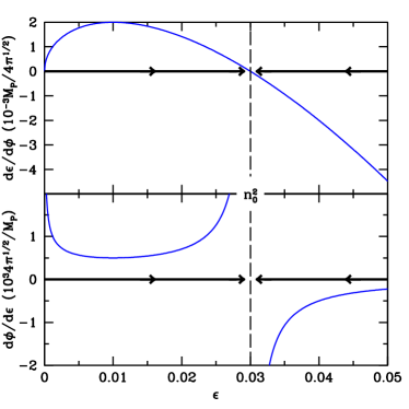
Figure 3: The values of $d\epsilon/d\phi$ and $d\phi/d\epsilon$ for an assumed value of $n_{0}^{2}=0.03$. Notice that the sign of the derivatives implies that for $\epsilon\rightarrow n_{0}^{2}$ the value of the field tends toward infinity.

We have already seen that if $\epsilon=\eta$, then $\epsilon$ is a constant given by $\epsilon_{0}=n_{0}^{2}$, and that this fixed point corresponds to power-law inflation generating a $k$-independent density spectral index given by $n(k)=1-2n_{0}^{2}$. This result also allows one to reconcile the apparent contradictory requirements for the generation of a Harrison–Zel’dovich power spectrum stemming from the lowest-order slow-roll approximation condition, $\eta=2\epsilon$, and by power-law inflation definition $\epsilon=\eta=\xi=\cdots=n_{0}^{2}$. One can see once again that a Harrison–Zel’dovich power spectrum can be generated by power-law inflation in the limit $n_{0}^{2}\rightarrow 0$ (i.e. $p\rightarrow\infty$), which corresponds to pure de Sitter expansion Lidsey:1995np .

Turning our attention to the case $\epsilon_{0}\neq n_{0}^{2}$, it is easier to consider the derivative of $\phi$ with respect to $\epsilon$,

$$\frac{d\phi}{d\epsilon}\simeq\frac{M_{{\rm p}}}{4\sqrt{\pi}}\frac{1}{\sqrt{\epsilon}(n_{0}^{2}-\epsilon)},$$ (72)

which is also shown in Fig. 3. The interesting feature here is that the point $\epsilon=n_{0}^{2}$ represents an asymptote of $d\phi/d\epsilon$: integrating it on either side with $\epsilon\rightarrow n_{0}^{2}$ yields a logarithmically-diverging field. This necessarily implies that the value of the field, parametrized by $\epsilon$, will tend to infinity while $\epsilon$ tends toward $n_{0}^{2}$. Remembering that Eq. (55) is integrated to yield $\phi(\epsilon)$, it is then possible to note that the three distinct regions $\epsilon<n_{0}^{2}$, $\epsilon=n_{0}^{2}$ and $\epsilon>n_{0}^{2}$ will give rise to three different dynamical behaviors for $\phi$, which, once inserted in the expression for $V(\epsilon)$, are able to produce the same density perturbation spectral index. The apparent puzzle that arose at the end of Sec. IV.2.1 has therefore been solved: there are in fact two potentials, and both their domains are $\phi\in[0,\infty[$. It is now possible to understand that each one of them – together with power law inflation – is able to generate the desired power spectrum, depending on the initial condition chosen for the slow-roll parameter.

V.2 The $n_{0}^{2}\leq 0$ case

The cases $n_{0}^{2}=0$ and $n_{0}^{2}<0$ are similar. From Eq. (55) we see that, independent of $\epsilon_{0}$, the value of $\epsilon$ will tend toward zero as inflation proceeds. In the $n_{0}^{2}<0$ case the solution derived Sec. IV.2 is the only one available, while in the special case $n_{0}^{2}=0$ (Harrison–Zel’dovich) it is possible to claim that two different inflationary potentials will be able to generate such a power spectrum: the flat one giving rise to the classical de Sitter expansion, and the one derived in Sec. IV.1.1, whose first term is proportional to $\phi^{-2}$.

VI Discussion

The analysis that has been carried out shows that inflaton potentials yielding the Harrison–Zel’dovich flat spectrum can be determined to lowest-order and next-order approximation in the slow-roll parameters. Similarly, potentials producing a $k$-independent spectral index slightly different from unity have been derived to lowest-order and to next-order.

It is also possible to speculate that the same procedure can be carried out to any order of expansion in the slow-roll parameters. This is because the implications of the spectral index $k$-independence are not as trivial as they may seem at first glance. Notice in fact that every time a higher approximation order is assumed, new slow-roll parameters will appear in the expression for the spectral index: going from lowest-order to next-order, for example, $\xi^{2}$ was introduced. This is hardly surprising, though, because these new parameters just correspond to higher derivatives of $V(\phi)$ or $H(\phi)$ (whatever is the degree of freedom chosen to express the slow-roll parameters) and a higher order treatment necessarily needs to take into account more derivative terms of the potential. However, the requirement of the spectral index to be $k$-independent implies not only a particular value for $n(k)$ but also that all its derivatives are equal to zero:

$$\frac{d^{i}n(k)}{d(\ln k)^{i}}=0,\textrm{ with }i=1,2,...$$ (73)

Furthermore, the expression for the ${(l_{0}-1)}^{th}$ derivative of the spectral index contains slow-roll parameters up to the $l_{0}^{th}$ one. So once the approximation order $l_{0}$ is chosen, the problem is characterized by $l_{0}+1$ parameters and $l_{0}$ equations of constraint relating them. This allows the expression of all the slow-roll parameters $\lambda_{H}^{l}$ as functions of $\epsilon$. The choice of $\epsilon$ is not arbitrary, because once the expression for $(\eta-\epsilon)$ appropriate for the approximation level assumed is derived, the exact expressions for $d\epsilon/d\phi$ and for $d\ln V/d\epsilon$, Eqs. (20) and (22), can be exploited to compute $\phi$ and $V$ as functions of $\epsilon$ thus yielding the map $\phi\rightarrow V(\phi)$.

References

(1)
A. Guth,
Phys. Rev. D23, 347 (1981)
(2)
D. H. Lyth and A. Riotto,
Phys. Rep. 314 1 (1999);
A. Riotto,
hep-ph/0210162; W. H. Kinney, astro-ph/0301448.
(3)
V. F. Mukhanov and G. V. Chibisov,
JETP Lett. 33, 532 (1981).
(4)
S. W. Hawking,
Phys. Lett. 115B, 295 (1982).
(5)
A. Starobinsky,
Phys. Lett. 117B, 175 (1982).
(6)
A. Guth and S. Y. Pi,
Phys. Rev. Lett. 49, 1110 (1982).
(7)
J. M. Bardeen, P. J. Steinhardt, and M. S. Turner,
Phys. Rev. D28, 679 (1983).
(8)
S. Dodelson, W. H. Kinney, and E. W. Kolb,
Phys. Rev. D56, 3207 (1997).
(9)
W. H. Kinney,
Phys. Rev. D58, 123506 (1998).
(10)
W. H. Kinney, A. Melchiorri, A. Riotto,
Phys. Rev. D63, 023505 (2001);
S. Hannestad, S. H. Hansen, and F. L. Villante,
Astropart. Phys. 17 375 (2002);
S. Hannestad, S. H. Hansen and F. L. Villante,
Astropart. Phys. 16, 137 (2001);
D. J. Schwarz, C. A. Terrero-Escalante, and A. A. Garcia,
Phys. Lett. B517, 243 (2001);
X. Wang, M. Tegmark, B. Jain and M. Zaldarriaga, Phys. Rev. D68, 123001
(2003).
(11)
H. V. Peiris et al. [WMAP collaboration], Astrophys. J. Supp. 148,
213 (2003).
(12)
V. Barger, H. S. Lee and D. Marfatia, Phys. Lett. B565, 33 (2003).
(13)
W. H. Kinney, E. W. Kolb, A. Melchiorri, and A. Riotto,
hep-ph/0305130.
(14)
S. M. Leach and A. R. Liddle, Phys. Rev. D68, 123508 (2003).
(15) C. L. Bennett et al. [WMAP collaboration], Astrophys. J.
Supp. 148, 1 (2003); D. N. Spergel et al. [WMAP collaboration],
Astrophys. J. Supp. 148, 175 (2003).
(16)
M. Tegmark et al. [SDSS Collaboration],
astro-ph/0310725.
(17)
M. Tegmark et al. [SDSS Collaboration], astro-ph/0310723.
(18)
A. R. Liddle, astro-ph/0401198.
(19)
F. Lucchin and S. Matarrese,
Phys. Rev. D32, 1316 (1985);
Phys. Lett. B164, 282 (1895).
(20) P. J. Steinhardt and M. S. Turner, Phys. Rev. D29, 2162
(1984); E. W. Kolb and M. S. Turner, The Early Universe,
Addison–Wesley, Redwood City (1990).
(21) D. S. Salopek and J. R. Bond, Phys. Rev D42, 3936 (1990).
(22) A. R. Liddle, P. Parsons, and J. D. Barrow, Phys. Rev.
D50, 7222 (1994).
(23)
E. D. Stewart and D. H. Lyth,
Phys. Lett. B302, 171 (1993).
(24)
J. E. Lidsey, A. R. Liddle, E. W. Kolb, E. J. Copeland, T. Barreiro, and M.
Abney,
Rev. Mod. Phys. 69, 373 (1997).
(25)
E. Ayón-Beato, A. García, R. Mansilla, and C. A.
Terrero-Escalante, Phys. Rev. D62 103513 (2000); C. A.
Terrero-Escalante, E. Ayón-Beato, and A. García, Phys.
Rev. D64 023503 (2001).
(26)
J. D. Barrow and A. R. Liddle, Phys. Rev. D47, 5219 (1993).