Efficiency Gains from Time Refinement on AMR Meshes and Explicit Timestepping

Abstract

Block-structured AMR meshes are often used in astrophysical fluid simulations, where the geometry of the domain is simple. We consider potential efficiency gains for time sub-cycling, or time refinement (TR), on Berger-Collela and oct-tree AMR meshes for explicit or local physics (such as explict hydrodynamics), where the work per block is roughly constant with level of refinement. We note that there are generally many more fine zones than there are coarse zones. We then quantify the natural result that any overall efficiency gains from reducing the amount of work on the relatively few coarse zones must necessarily be fairly small. Potential efficiency benefits from TR on these meshes are seen to be quite limited except in the case of refining a small number of points on a large mesh — in this case, the benefit can be made arbitrarily large, albeit at the expense of spatial refinement efficiency.

1 Introduction

1.1 Block-Structured AMR

Adaptive mesh refinement on rectangular grids (henceforth AMR) was introduced in bergeroliger , and improved for conservation laws in bergercollela , henceforth BC89. In the patch-based meshes of the sort described in BC89, the patches increase in resolution by a fixed even integer factor $N$. One can place a finer patch anywhere in the domain of a ‘parent’ patch of one fewer level of refinement. A patch is not required to have only a single parent, but must be completely contained within patches of the next lowest level of refinement. Note that these meshes are non-conforming; the face of a zone in a parent patch will abut $N$ faces in the child patch. A final restriction in the nesting of the meshes is that there must be at least one zone of the next lower level refinement about the perimeter of a patch.

Another mesh we will consider here is an oct-tree mesh (quad-tree in 2-d, binary tree in 1d), such as is implemented in the Paramesh package paramesh used in the Flash code flashcode . This oct-tree mesh is a more restrictive version of an $N=2$ patch-based mesh as described in BC89. If a block needs additional resolution somewhere in its domain, the entire block is halved in each coordinate direction, creating $2^{d}$ children, where $d$ is the dimensionality. Leaf blocks are defined to be those blocks with no children, and are thus at the bottom of the tree — they are the finest-resolved blocks in their region of the domain. Frequently, only leaf blocks are evolved to compute the solution to the equations, since a refined parent block’s domain is completely spanned by its children.

The only difference between the two meshing approaches of immediate interest is the resulting different refinement patterns. We will use ‘patch’ and ‘block’ interchangeably in this paper.

1.2 Time Refinement

In BC89, the timestep set by the data on the finest mesh is used to evolve that data, and data on the coarser meshes is evolved at a multiple thereof so that there is a constant ratio at each level $l$ of $\Delta t_{l}$ to $\Delta x_{l}$. The assumption here is that there is one roughly spatially constant characteristic speed throughout the entire domain, so that the maximum allowable timestep at any given resolution is directly proportional to the size of the mesh for any given block or patch. When coupled with the assumption in structured AMR of some fixed jump in refinement between levels, this makes for a very natural time evolution algorithm, shown pictured in Figure 1 for a mesh with three different levels of refinement, with resolution jumps by constant factors of $N$; shown is $N=2$.

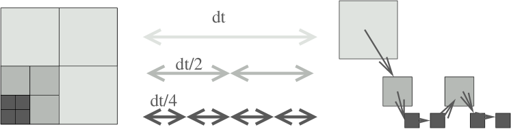
Figure 1: A structured AMR mesh containing blocks at three different levels of refinement, showing the order of operations (far right) of an explicit time evolution algorithm. The largest block is evolved at the system timestep, and smaller blocks are subcycled at smaller timesteps. Between evolution at different levels of the mesh, time averaging and flux corrections must be done — these are not shown here.

Here the largest blocks are evolved at some system timestep $dt$, and smaller blocks are ‘subcycled’ at proportionally smaller timesteps. This defines a ‘work function’ for each block; the finest blocks must be evolved every sub-timestep so we take their work value to be 1 times the number of zones in the block or patch; the blocks one level of refinement ‘up’ need only be evolved every $N$ sub-timesteps, so that their work value is $1/N$ times the number of zones, etc. The work function for an entire mesh is the sum of the work values of each block or patch in the mesh.

There are costs associated with this time refinement (hereafter TR). Memory is needed to store information at multiple timesteps. There are overheads from extra copies and time-centering of fluxes. The modified time-structure of work leads to load-balance issues in parallel jobs. Further complicating parallel performance is increased communication complexity (although, it is to be pointed out, not necessarily increased communication).

Nonetheless, one might hope that these costs are outweighed by the time savings of not evolving large blocks at unnecessarily small timesteps; in the example of Figure 1, of evolving the larger blocks at timesteps of $dt$ or $dt/2$ instead of $dt/4$. As a first step to quantify the possible benefits, we estimate the reduction in computational cost in simple cases §2. We then use the same approach to examine meshes from simulations performed with a tree-based mesh in §3. In our final section we summarize our results.

2 Simple Mesh Configurations

Here we calculate both the number of evolved blocks in a simple mesh, and a weighted sum representing the ideal amount of work done by a TR method, using the work function described in the previous section. We then calculate a work ratio, $R$ — the amount of work that would be done by the idealized TR divided by that done with no time refinement. With no time refinement, each block must be stepped through each sub-timestep, so that the amount of work done is simply the number of blocks; thus, the work ratio is simply (TR work function)/(number of blocks). For $R=1$, there is no reduction in work; for $R<1$, TR reduces the amount of computational work.

One can interpret the work ratios as performance metrics for the TR, assuming that – all physics benifits from the time subcycling in proportion to the reduction in number of blocks evolved each step; the memory overhead from TR is unimportant; all larger blocks actually can be evolved at timesteps of larger size in proportion to their physical size; there is no single-processor overhead from TR from memory copies or flux averaging; there is no parallel overhead from increased complexity in communications; and there is no parallel from increased load-balancing issues.

2.1 Point refinement

The best case for efficiency gains for spatial refinement is clearly one isolated point of refinement. For a patched-based mesh, we imagine refinements as shown on the left of in Figure 2.

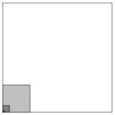
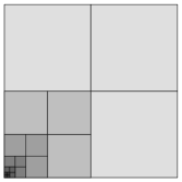
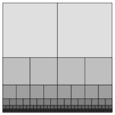
Figure 2: Fully refining a zero-thickness point with an idealized patch-based type mesh (far left) and an oct-tree mesh (left); Fully refining an interface with a patch-based mesh (right) and oct-tree mesh (far right). For the patch-based mesh, it is assumed that a patch can be placed anywhere on existing patches, with some fixed integral increase in resolution (shown here is $N=4$, $L=3$). For the oct-tree mesh, $N$ is fixed at 2, and shown is $L=5$.

We begin with domains of length one in all directions. The completely unrefined domain is defined to be at level $l=1$ of refinement. Consider placing increasingly fine patches at the corner, until we resolved the finest scale $\Delta x$ we wished. If this requires $L-1$ more levels of refinement, each decreasing the zone size by an integer factor $N$, then we have $\Delta x\sim(1/N)^{L-1}$. We will assume $\Delta x\ll 1/2$.

We consider the mesh in terms of the smallest uniform unit — for the oct-tree mesh, this is a single block, which will be of size $n_{x}\times n_{y}\times n_{z}$ zones. For the patch-based mesh, since the patches can be of arbitrary size (and shape), we consider zones individually. (Because we are not modelling guardcell filling, we can safely ignore the fact that these zones are actually components of patches). Thus, in the results given below, an oct-tree mesh with (say) $8\times 8$-zone blocks at a maximum refinement $L=5$ has the same resolution as a patch-based mesh with $L=8$.

The amount of work required by a non-TR code with only explicit or local solves will, by assumption, be the same for each block, so that $W_{\mathrm{noTR}}=N_{\mathrm{blocks}}$. The amount of work with time refinement, $W_{\mathrm{TR}}$, will be a weighted sum of blocks. For the pointwise-refined patch mesh, the number of blocks will simply be $N_{\mathrm{blocks}}=L$, as there is only one block per level. The amount of TR work is

$$W_{\mathrm{TR}}=\sum_{l=1}^{L}1\cdot\left(\frac{1}{N}\right)^{L-l}\sim\frac{N}{N-1}.$$ (1)

Thus the work ratio will be

$$R=\frac{W_{\mathrm{TR}}}{W_{\mathrm{noTR}}}=\frac{W_{\mathrm{TR}}}{N_{\mathrm{blocks}}}=\frac{N}{L(N-1)}.$$ (2)

For ideal spatial AMR, where one can do all the refinement with only one jump, $L=2$, and so the amount of work done by a TR algorithm is bounded from below at $1/2$ of the non-TR work. At the other limit, for a much less aggressive AMR with $N=2$, then the work can be made an arbitrarily small fraction of the non-TR algorithm, with $R=2/L$ — but note that this work ratio is achieved only by operating on $L/2$ times as many blocks as in the best case for spatial AMR.

The oct-tree meshes refining on a point is shown on the right of Figure 2. In this case, there are $2^{d}$ highest refined blocks in the corner, with the rest of the $2^{d}-1$ surrounding blocks at the next highest refinement, surrounded by the $2^{d}-1$ surrounding blocks at the next highest level of refinement, and so on.

Thus the total number of leaf blocks is

$$N_{\mathrm{blocks}}=(2^{d})+\sum_{l=L-1}^{1}{\left(2^{d}-1\right)}=2^{d}(L-1)-L+2$$ (3)

Weighting them by the amount of work,

$$W_{\mathrm{TR}}=(2^{d})+\sum_{l=L-1}^{1}{\left(\frac{(2^{d}-1)}{2^{(L-l)}}\right)}\sim 2^{(d+1)}-1$$ (4)

making the work ratio

$$R=\left\{\begin{array}[]{cl}3/L&1d\\ 7/(3L-2)&2d\\ 15/(7L-6)&3d\end{array}\right.$$ (5)

As with the patch-based result, this ratio goes to zero for arbitrarily large $L$. These results are similar to the $N=2$ patch-based result, but TR performs better here, and the spatial refinement worse — both of these are due to the fact that the oct-tree mesh generates more intermediate-level blocks.

2.2 Planar Interface Refinement

The refinement of an interface is shown on the right of Figure 2. In the patch-based case, we continually place a grid of $N$-by-1 (in 2d) or $N^{2}$-by-1 (in 3d) patches along the interface, until the required resolution is achieved.

In this case, performing the same calculation as in the previous section, one obtains

$$R\approx 1-\frac{N-1}{N^{d}-1}.$$ (6)

Here, there is a fixed lower bound for the amount of work the TR can achieve. In the spatially-optimal large-$N$ limit, no work is saved at all: $R\rightarrow 1$. At the other limit, for $N=2$, in 2d, $R\rightarrow 2/3$; in 3d, $R\rightarrow 6/7$.

In the oct-tree mesh we begin with one block at the coarsest level. It must be divided into 4 in this 2D example, or, in general, $2^{d}$. Half of these blocks will be further refined. This continues until we reach the maximum level of refinement. The work ratio one finds is

$$R=\left\{\begin{array}[]{cl}7/9&2d\\ 45/49&3d\end{array}\right.$$ (7)

In the point-refinement case of the previous subsection, a point of zero volume needed to be refined; as a result, there were the same number of blocks at each level, and thus a significant time savings could be obtained by doing less work at the coarser blocks. However, as we begin to see here, as soon as a non-trivial volume of the mesh needs to be refined, there is significantly less savings to be had.

2.3 Circular Region Refinement

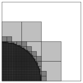
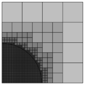
Figure 3: Fully refining the interior of a circle, shown here with radius of $0.49$ of the box size, with an idealized patch-based type mesh (left) and an oct-tree mesh (right). The patch-based mesh shown has $L=3$ and $N=4$. For the oct-tree mesh, $N$ is fixed at 2, and shown is $L=6$.

The loss of efficiency gains when a non-zero fraction of the mesh must be refined is even clearer when a region, rather than an interface, is fully refined. In Fig. 3 we see the results of fully refining the interior of a quarter-circle with the center at one of the corners of the domain. Clearly, the number of finest blocks greatly outnumber intermediate or large blocks, so one might guess that there is very little efficiency gain that can be had from reducing work on the larger blocks.

	L=2	3	4	5	6	7	8
r = 0.0	0.786	0.625	0.510	0.426	0.363	0.316	0.279
0.1	0.786	0.625	0.510	0.510	0.638	0.765	0.879
0.2	0.786	0.625	0.625	0.714	0.806	0.895	0.940
0.5	0.962	0.843	0.851	0.888	0.931	0.963	0.981
0.9	1.	0.973	0.962	0.962	0.973	0.982	0.989

Table 1: Work ratio for a 2d Oct-tree mesh with a circular region of radius $r$ (in units of the domain) completely refined.

Because in this case the refinement pattern is complicated enough that the process must be iterated to check that each zones neighbors are no further than one level of refinement appart, we do not provide analytic work ratios. Tables 1 and 2 show the work ratios for an Oct-Tree mesh and an $N=2$ patch-based mesh in refining a circular region of radius $r$. Again, the $r=0$ results reproduce the expected point refinement, but as soon as a non-zero radius must be refined, the efficiency gains drop significantly further than in the case of only refining an interface, as more small blocks are needed to refine a region than the interface. In Table 2 we also show results for the patch based mesh with $N=4$; we see as in previous sections that for the same resolution, increasing $N$ (which increases the spatial efficiency of AMR) decreases the possible gains from time subcycling.

	N=2, L= 2	3	4	5	6	7	8	N=4, L=2	3	4
r = 0.0	0.583	0.468	0.387	0.328	0.283	0.249	0.221	0.438	0.332	0.510
0.1	0.583	0.468	0.444	0.552	0.658	0.754	0.802	0.719	0.891	0.510
0.2	0.583	0.548	0.618	0.694	0.768	0.806	0.833	0.812	0.914	0.625
0.5	0.75	0.737	0.763	0.798	0.825	0.840	0.848	0.896	0.938	0.851
0.9	0.847	0.827	0.826	0.833	0.842	0.848	0.852	0.938	0.947	0.962

Table 2: Work ratio for a 2d patch-based mesh, $N=2$ and $N=4$, with a circular region of radius $r$ (in units of the domain) completely refined.

3 Meshes from simulations

The calculations of the previous section are for very simple refinement geometries. In this section, we apply the same work function used in §2 to the output of previous actual AMR simulations which use oct-tree based meshes for AMR. We continue to assume the same idealized performance results of the previous section.

We begin with examining results from a standard test problem, a Sedov explosion sedov , as included with the Flash code and described in flashcode . In this simulation, a high pressure at a point causes a spherical shock wave to expand outwards; this is analogous to the circular region analysis of the previous section. The adaptive mesh for different stages of this simulation in 2d are shown in 4.

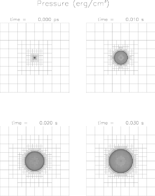
Figure 4: The mesh of a Sedov explosion, from the Flash setup test described in flashcode , with a maximum of 8 levels of refinement. Each block shown contains $8\times 8$ zones.

Results from the meshes shown are tabulated in Table 3. The number of blocks listed in the table is the number of ‘leaf’ blocks – e.g., the blocks that are actually evolved. Also given in the table is the work ratio ($R$) and the work ratio of spatial AMR to a uniform mesh at the highest resolution ($R_{\mathrm{AMR}}=W_{\mathrm{noTR}}/W_{\mathrm{uniform}}$). We include $R_{\mathrm{AMR}}$ to compare the relative importance of performance gains for the spatial refinement and the time subcycling.

TR provides a large performance gain initially, when there is only one point that is refined. However, consistant with previous results, immediately as the point becomes a region of non-zero measure, idealized performance gains drop to $30\%$–$10\%$. Regardless of the refinement, the TR provides a very small performance enhancement compared to that of the spatial refinement.

time	$N_{\mathrm{blocks}}$	$R$	$R_{\mathrm{AMR}}$
0.00	256	0.426	0.0156
0.01	892	0.805	0.0544
0.02	1552	0.835	0.0947
0.03	2092	0.874	0.127

Table 3: Results from simulations of a Sedov explosion. Listed at different evolution times are the number of leaf blocks in the mesh, the work ratio, and the work ratio for spatial AMR to uniform grid.

The reason for the small predicted efficiency gains, consistent with the discussion of the previous section, is that there quickly become more fine blocks than coarse blocks in the simulation. By the last frame shown in Figure 4, there are no blocks being evolved at the the coarsest level of refinement, and indeed 80% of the blocks are at the highest level of refinement. Thus, even if all other blocks required zero work to evolve, we could only achieve a $20\%$ speedup.

Next we consider an interface problem – a 2d detonation that will eventually undergo a cellular instability. These simulations are from results published in celldet2d . A mesh is shown in Figure 5. This corresponds almost exactly to the idealized interface problem of the previous section, but here the domain is very long in one direction, increasing the number of low-cost coarsest blocks in the domain. This change in distribution of blocks means that this problem can benefit more from TR. The numerical results are shown in Table 4.

Figure 5: Half of the domain for the initial condition of a detonation, where the long domain is refined nowhere except at a sharp interface. The domain originally consists of a top-level mesh of $1\times 20$ blocks. This mesh is then refined at an interface. Shown is the meshes 6, zoomed in near the interface. Not shown are 10 coarsest blocks to the right.

Max refinement	$N_{\mathrm{blocks}}$	$R$	$R_{\mathrm{AMR}}$
4	62	0.633	0.0484
5	110	0.688	0.0215
6	206	0.727	0.0101
7	398	0.751	0.00486

Table 4: Results from initial conditions for a 2-d detonation problem, as in Figure 5. $R$ is less than the $7/9$ calculated in the previous section, because of the large number of extra coarsest blocks added to the domain.

Here we see TR’s efficiency gains actually decrease with increasing resolution, and also see a familiar pattern of TRs efficiency gains going in the opposite direction of spatial AMR efficiency gains. Even at the resolution where TRs efficiency gains are largest, they are much smaller than the improvement from using spatial AMR.

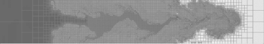
Figure 6: Development of Rayleigh-Taylor instability at 3 epochs, from simulations presented in vandv . These are fairly high-resolution simulations, with a maximum of 8 levels of refinement on a top-level mesh with $6\times 1$ coarsest blocks.

We next consider the development of the Rayleigh Taylor instability. (Figure 6). This is an interface problem, but in this set of simulations, the center region of the box is resolved to ensure resolution of the velocity perturbations in the region near the interface. Because this region is fully refined, many ‘full cost’ finest blocks are added. This decreases the scope of improvement from TR, as seen in Table 5.

time	$N_{\mathrm{blocks}}$	$R$	$R_{\mathrm{AMR}}$
0.0	33150	0.993	0.337
1.8	33150	0.993	0.337
3.6	60816	0.987	0.619

Table 5: Numerical results from simulations of a Rayleigh-Taylor instability, shown in Figure 6.

4 Conclusion

We have considered efficiency gains for time subcycling for explict or local physics. In these cases the work per block is roughly constant. Further, in most cases there are many more fine blocks than coarse blocks — this is due to simple geometry, as a mesh that refines a significant fraction of its domain will be strongly weighted in favour of small blocks, which must be evolved at a small timestep. Thus, Any attempt to improve performance by focusing on the relatively few larger blocks can only reduce a small fraction of the work that needs to be done to evolve the system one timestep. On the other hand, in studies where only a small number of points in a large domain must be fully resolved, there may be significant efficiency gains from TR methods. Some cosmological hydrodynamical simulations normanextreme are examples of this situation.

We have not considered here accuracy; taking fewer timesteps may increase accuracy with some solvers, although this isn’t clear for moderately time-accurate algorithms having errors of $O({\Delta t}^{p})$, $p>1$; further, the coarsely refined regions which would benefit from the fewer timesteps are presumably coarsely refined because the overall solution quality is less sensitive to the error in those regions than it is to that of the highly refined parts of the domain. We also do not consider global or implicit solves, where the timestepping algorithm in Fig. 1 must be modified. Global or implicit solves will, depending on the methods used, change the amount of work done per block at different levels of refinement, which can change the results given here considerably.

We have modelled only computational cost in this work. Most of the other costs, cf. §2, work to decrease the efficiency gains of TR. One unmodelled effect that could increase the gains is the reduction of guardcell fills on large blocks. For the oct-tree mesh, where the number of zones per block is fixed, the reduction in guardcell filling work is reduced in the same way as the computational work, so that our conclusions are unchanged. For the patch-based mesh, the effect on the guardcell filling will be dependant on the shape of the refined region and the algorithm used for merging patches of the same refinement level, so that it is difficult to say anything in general.

Thus, block-structured TR significantly enhances performance of local or explicit physics solvers only under fairly narrow circumstances. In circumstances where TR is unlikely to produce much performance enhancement, the added code complexity, memory overhead, and parallel load-balancing issues may make the costs of the technique exceed its benefits.

The authors thank B. Fryxell for useful discussions with this paper, and K. Olson with his help with Paramesh over the past years. We thank A. Calder for data from RT simulations, and F. X. Timmes for data from cellular detonation simulations. We thank T. Plewa, G. Weirs, R. Kirby, and R. Loy for suggesting this work. Support for this work was provided by the Scientific Discovery through Advanced Computing (SciDAC) program of the DOE, grant number DE-FC02-01ER41176 to the Supernova Science Center/UCSC. LJD was supported by the Department of Energy Computational Science Graduate Fellowship Program of the Office of Scientific Computing and Office of Defense Programs in the Department of Energy under contract DE-FG02-97ER25308.

The Flash code is freely available at http://flash.uchicago.edu/.

References

- [1] T. Abel, G. L. Bryan, and M. L. Norman. The Formation of the First Star in the Universe. Science, 295:93–98, January 2002.
- [2] M. J. Berger and P. Collela. Local adaptive mesh refinement for shock hydrodynamics. J. Comp. Phys., 82:64–84, 1989.
- [3] M. J. Berger and J. Oliger. Adaptive mesh refinement for hyperbolic partial differential equations. J. Comp. Phys., 53:484–512, 1984.
- [4] A. C. Calder, et al. On validating an astrophysical simulation code. ApJSS, 143:201–230, 2002.
- [5] B. Fryxell, et al. FLASH: An Adaptive Mesh Hydrodynamics Code for Modeling Astrophysical Thermonuclear Flashes. ApJSS, 131:273–334, November 2000.
- [6] P. MacNeice, et al. Paramesh: A parallel adaptive mesh refinement community toolkit. Computer Physics Communications, 126:330–354, 2000.
- [7] L. I. Sedov. Similarity and Dimensional Methods in Mechanics. Academic Press, New York, 1959.
- [8] F. X. Timmes, et al. On the Cellular Structure of Carbon Detonations. ApJ, 543:938–954, November 2000.