Ionizing radiation fluctuations and large-scale structure in the Lyman-alpha forest

Abstract

We investigate the large-scale inhomogeneities of the hydrogen ionizing radiation field in the Universe at redshift $z=3$. Using a raytracing algorithm, we simulate a model in which quasars are the dominant sources of radiation. We make use of large scale N-body simulations of a $\Lambda$CDM universe, and include such effects as finite quasar lifetimes and output on the lightcone, which affects the shape of quasar light echoes. We create Ly$\alpha$ forest spectra that would be generated in the presence of such a fluctuating radiation field, finding that the power spectrum of the Ly$\alpha$ forest can be suppressed by as much as $15\%$ for modes with $k=0.05-1\;h^{-1}{\rm Mpc}$. This relatively small effect may have consequences for high precision measurements of the Ly$\alpha$ power spectrum on larger scales than have yet been published. We also investigate a second probe of the ionizing radiation fluctuations, the cross-correlation of quasar positions and the Ly$\alpha$ forest. For both quasar lifetimes which we simulate ($10^{7}$ yr and $10{{}^{8}}$yr), we expect to see a strong decrease in the Ly$\alpha$ absorption close to other quasars (the “foreground” proximity effect). We then use data from the Sloan Digital Sky Survey First Data Release to make an observational determination of this statistic. We find no sign of our predicted lack of absorption, but instead increased absorption close to quasars. If the bursts of radiation from quasars last on average $<10^{6}$ yr, then we would not expect to be able to see the foreground effect. However, the strength of the absorption itself seems to be indicative of rare objects, and hence much longer total times of emission per quasar. Variability of quasars in bursts with timescales $>10^{4}$yr and $<10^{6}$ yr could reconcile these two facts.

1. Introduction

The Ly$\alpha$ forest is a useful probe of the structure of the high redshift Universe. Over most of the volume of space, the hydrogen responsible for Ly$\alpha$ absorption is in photoionization equilibrium with a background radiation field. The optical depth for Ly$\alpha$ absorption at a given point in space is related simply to the density (see e.g., Bi 1993, Hui, Gnedin & Zhang 1997, Croft et al. 1997) and also inversely to the intensity of the ionizing radiation. The correlation of Ly$\alpha$ absorption with the density field has been much studied, including its use as a probe of matter clustering (e.g., Hui 1999, Nusser & Haehnelt 1999, McDonald et al. 2000, Viel et al. 2002). The inhomogeneities of the radiation field however have not been much examined in this context (although see the recent work of Meiksin & White 2003ab). In this paper we present a method for predicting the large-scale fluctuations in the radiation field and their effect on Ly$\alpha$ forest spectra and their statistical properties.

The study of the reionization of the Universe using radiative transfer in simulations is a rapidly growing field (e.g., Abel et al. 1999, Gnedin 2000, Ciardi et al 2001, Sokasian et al. 2001, Razoumov et al. 1999,2002) At redshifts soon after the reionization epoch, the Universe is still relatively optically thick, and the fluctuations in the radiation field are expected to be very large (e.g., Meiksin & White 2003b). As the Universe expands, however, the dilution of the density field reduces the number density of neutral hydrogen atoms also, so that by $z=3$ (the epoch we will study in this paper), the mean free path of ionizing photons is expected to be $\lower 2.15277pt\hbox{$\;\buildrel>\over{\sim}\;$}100\;h^{-1}{\rm Mpc}$ comoving (Haardt and Madau 1996, hereafter HM96). If the dominant sources of photons are rare objects such as quasars, then only a few will lie within each attentuation radius (the mean distance to reach a unit optical depth for absorption). Fluctuations in the radiation field will be relatively gentle, but occur on large scales, comparable to the mean separation between sources (e.g., Zuo 1992a, Fardal and Shull 1993). This epoch is difficult to treat accurately with simulations, because one would like to resolve both the small scale clumping of the IGM and the large distance between rare sources. In this paper we will make use of hybrid approach which combines large dark matter simulations with optical depths calibrated from a high resolution hydrodynamic run.

The intensity fluctuations in the ionizing background have been studied using an analytical technique by Zuo (1992a,b) for randomly distributed sources. The effect on the Ly$\alpha$ forest was also studied by Fardal and Shull (1993) who used the same techniques, as well as Monte Carlo simulations, again for randomly distributed clouds. Croft et al. (1999) made a simple study of the effect of such fluctuations on the recovery of the matter power spectrum from the Ly$\alpha$ forest, finding no significant effect on the small scales ($k>0.2\;h\;{\rm Mpc}^{-1}$) then observationally accessible but a potentially interesting effect on large scales. All of these approaches assumed a uniform IGM which attentuates photons isotropically (no shadowing is possible), as well as ignoring the effect of finite source lifetimes. More recent work has been carried out by Gnedin and Hamilton (2002), in a small simulation volume ($4\;h^{-1}{\rm Mpc}$) at $z=4$, finding that fluctuations are negligible on these scales and below. Meiksin and White (2003ab) find strong fluctuations at $z>5$, combining a PM dark matter simulation with a uniform attentuation approximation.

The redshift ($z=3$) which we focus on in this paper is one for which much observational data is available, both for the Ly$\alpha$ forest, and for Lyman Break Galaxies (e.g., Adelberger et al. 2003, Steidel et al. 2003 ). The structure in the radiation field itself is expected to be quite interesting and complex, manifesting itself on much larger scales than the structures in the density field. We aim to investigate how the clustering of the Ly$\alpha$ forest will be influenced by the structure of the radiation field, which in turn depends on the lifetime of quasar sources, and the fractional contribution of quasars to the overall background radiation intensity. We will also investigate the Ly$\alpha$ forest absorption in lines of sight which pass close to foreground quasars (testing what is sometimes known as the foreground proximity effect). Here, close to the sources of radiation, the effect of inhomogeneities in the radiation field should manifest themselves most strongly. Comparison with observational measurements have the potential to constrain the source lifetime and possibly the geometry of space.

The paper is set out as follows. In §2, we describe the set of simulations which we will use. In §3 we describe our raytracing method which we we apply to the outputs of these simulations. We detail some properties of the resulting radiation field before describing our procedure for generating Ly$\alpha$ forest spectra in the presence of this field. In §4, we measure the power spectum of the Ly$\alpha$ forest flux in these spectra, and investigate its dependence on quasar lifetime, beaming of radiation, and the inclusion of light cone effects. In §5 we turn to the Ly$\alpha$ forest averaged around foreground quasars, showing simulation results. We also compute this statistic from the Sloan Digital Sky Survey First Data Release and carry out a comparison with the models. Our summary and discussion form §6.

2. Simulations

We will use N-body simulations of large-scale structure in order to create a framework involving sources and sinks of radiation. Our aim is to examine the statistical properties of the radiation field on large scales, and to make use of sparsely distributed sources (QSOs). Because of both these factors, we must use large simulation volumes, and we choose to run several realizations with different random phases. We also have run different box sizes with different mass resolutions in order to carry out a resolution study. The main set of simulations which we will use are dark matter only. In order to compute the optical depth to absorption for ionizing photons which pass through the simulation, we have adopted a hybrid approach, making use of an output of a full hydrodynamic simulation. We calibrate the optical depths associated with the dark matter in our large low resolution simulations using information from the high resolution hydro run. In the near future, when large box high resolution gas dynamical simulations become available, this hybrid approach will not be necessary.

The cosmological model we choose to simulate is a cosmological constant-dominated CDM universe, consistent with measurements from the WMAP satellite (Bennett et al. 2003, Spergel et al. 2003). We use with $\Omega_{\Lambda}=0.7$, $\Omega_{\rm m}=0.3$ $\Omega_{\rm b}=0.04$, and a Hubble constant $H_{0}=67{\rm\;km\;s^{-1}}\;{\rm Mpc}^{-1}$. The initial linear power spectrum is cluster-normalized with a linearly extrapolated amplitude of $\sigma_{8}=0.9$ at $z=0$.

2.1. Collisionless dark matter only

As stated above, we use dark matter only simulations for most of the work in this paper, which were run with the $P^{3}M$ code of Efstathiou et al. (1985). We have three sets of simulations, each with $200^{3}$ particles, and within each set run 5 realizations with different random phases. Unless stated otherwise, our results will be averages over the 5 realizations in each case. Our three sets of simulations have different box sizes and force resolutions. The box sizes are $500\;h^{-1}{\rm Mpc}$, $250\;h^{-1}{\rm Mpc}$ and $125\;h^{-1}{\rm Mpc}$ for what we term the “d500”, “d250” and “d125” sets. Their comoving force resolutions are $130h^{-1}{\rm kpc}$, $65h^{-1}{\rm kpc}$ and $33h^{-1}{\rm kpc}$ respectively, and they were all run from redshift $z=24$ to redshift $z=3$. The mass per particle for the runs is $1.3\times 10^{12}h^{-1}{\rm M_{\odot}}$ for the d500, $1.6\times 10^{11}h^{-1}{\rm M_{\odot}}$ for d250, and $2.0\times 10^{10}h^{-1}{\rm M_{\odot}}$ for d125.

2.2. Hydrodynamic simulation

We make use of the $z=3$ simulation output of the simulation described in White, Hernquist & Springel (2001), and Croft et al. (2002), and which was kindly provided by Volker Springel and Lars Hernquist. The box size is $33.5\;h^{-1}{\rm Mpc}$, and there are $300^{3}$ particles representing the gas, and $300^{3}$ representing the collisionless dark matter. The particle masses are therefore $1.5\times 10^{7}\,h^{-1}{\rm M_{\odot}}$ for the baryons and $1\times 10^{8}\,h^{-1}{\rm M_{\odot}}$ for the DM. The simulation was run using the smoothed particle hydrodynamics (SPH) code GADGET (Springel et al. 2001), and includes gas dynamics, cooling, and a multiphase treatment of star formation (see Springel & Hernquist 2003). Also, importantly, it was run including a uniform background of ionizing radiation, based on the results of HM96.

3. Method

Solving the general radiative transfer (RT) problem in the Universe is extremely challenging. Depending on the specific application, there are many shortcuts and innovative treatments which can be used. For example, when looking at growth of ionized regions in an optically thick neutral medium, the jump condition can be solved by casting along rays (Sokasian, Abel and Hernquist, 2001). A summary of the many different recent approaches to solving RT in the early Universe can be found in Section 1 of Maselli, Ferrara and Ciardi (2003).

In this paper, we are interested in the Universe at $z=3$, which is close to being optically thin, the mean free path of hydrogen ionizing photons being $\sim 100\;h^{-1}{\rm Mpc}$. The simplest approximation which can be made is that the attenuation of photons is isotropic about each source (e.g., Fardal & Shull 1993, Meiksin & White 2003). Once this assumption is dropped, it becomes necessary to deal with inhomogeneities in the optical depth, which we do using a raytracing approach. We make many other simplifications, however. For example, we do not carry out time dependent raytracing, so that the effect of earlier passages of radiation has no effect on the propagation of photons passing through the same region of space. As the fluctuations in the radiation field are small, and the time taken to recover to the mean neutral fraction is short, this is not unreasonable (we shall return to this later). Also, for simplicity, we deal with only one frequency, photons with energy 1 Rydberg.

3.1. Raytracing

Starting from sources of radiation (we describe their selection in §3.4 below), we trace the paths of photons through the static density field. We adopt a Monte Carlo approach (see e.g., Ciardi et al. 1999, Maselli et al. 2003), in which photons are emitted isotropically from sources (this is relaxed later for beamed sources). The directional polar angles are randomly picked from the distributions:

$$\theta=\arccos(1-2R_{\theta}),\ \phi=2\pi R_{\phi},$$ (1)

where $R_{\theta}$ and $R_{\phi}$ are random numbers from 0 to 1 (Ciardi et al. 1999).

Our approach during raytracing is not to first assign particle positions and densities to a grid, but instead integrate through the actual distribution of particle kernels. Our two reasons for doing this are to allow for more accurate shadowing from matter close to a source, and to be closer to the spirit of the Lagrangian technique involved. Since we are using dark matter particles as a proxy for gas, we first compute the optical depth for absorption for a given mass and density of dark matter. We calibrate the relation using the hydrodynamic simulation as follows. We first decide on a dark matter mass, which we take to be 8 of the dark matter only simulation particles. We then randomly pick cubes which contain this mass of dark matter plus gas from the hydrodynamic simulation, picking the centers at random and varying the side length so that they contain the required mass. We then shoot rays through the cube and for each one compute the optical depth for absorption by the neutral hydrogen present:

$$\tau(\nu)=\sigma(\nu)\int n_{HI}(x)dx,$$ (2)

where $\sigma(\nu)$ is the photoionization cross section. In this way, we make use of the high resolution of the hydrodynamic simulation which allows for clumping in the gas. Averaging over a number of sightlines ($N$) gives us an effective optical depth due to the cube with density $\rho$:

$$\tau_{\rm eff}(\rho)=-\ln\left(\frac{1}{N}\sum_{i=1}^{N}e^{-\tau_{i}}\right)$$ (3)

                                                                            

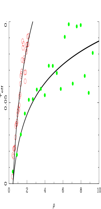
Figure 1.— The effective optical depth $\overline{\tau}_{\rm eff}$ seen by photon crossing through the neutral hydrogen associated with dark matter with the mass of 8 dark matter simulation particles, as a function of density in units of the mean. We show results from the d250 simulation (green points) and d500 simulation (red points), as well as parametric fits (solid lines).

In Figure 1, we show $\overline{\tau}_{\rm eff}(\rho)$ as a function of the density of matter in the cube, $\rho$. We show results for two dark matter masses, appropriate for 8 particles from the d500 and the d250 simulations. In the case of the d500 runs, the side length of a cube with the mean density that contains 8 particles is $5\;h^{-1}{\rm Mpc}$ (comoving). From Figure 1, we can see that at the mean density, $\overline{\tau}_{\rm eff}$ is $0.045$. This means that to reach an optical depth of 1 a photon with energy 1 Ryd. would have to move through a universe (uniform in density on scales $>5\;h^{-1}{\rm Mpc}$) a distance of $\sim 5\;h^{-1}{\rm Mpc}\times 1/0.045$, or $111\;h^{-1}{\rm Mpc}$.

This figure can be compared to the attenuation length $r_{0}$, which has been computed by many authors (e.g., Paresce et al. 1980) from the assumption of a universe uniform on large scales but populated with Ly$\alpha$ clouds and Lyman limit systems with different column densities, specified by matching with observations. Depending on the how the observations are interpreted and which cosmology is used, values of $r_{0}$ at $z=3$ (converted to comoving units) including 128 $\;h^{-1}{\rm Mpc}$ (HM96), $100-375\;h^{-1}{\rm Mpc}$ (Fardal and Shull 93) have been previously found. In Meiksin and White (2003a,b), $r_{0}$ was computed from dark matter based simulations of the Ly$\alpha$ forest with the addition of observational data on Lyman-limit systems which were unresolved by the simulation. Meiksin & White (2003a,b) find $r_{\rm att}\sim 210\;h^{-1}{\rm Mpc}$ at $z=3$. Our simulation result is therefore on the low end compared to other computed estimates, something which will tend to maximize the fluctuations in the radiation field. We note, however that because in our case we deal with an inhomogeneous absorbing medium, the effective attentuation length seen by photons from different sources and travelling in different directions will vary, and that the value of $r_{0}$ is not directly comparable. For example, in our $500\;h^{-1}{\rm Mpc}$ box runs (for QSOs with lifetimes $10^{7}$ yr - see later), we find that $30\%$ of photons are not absorbed after travelling half a box length, and those that are absorbed travel a mean distance of $80\;h^{-1}{\rm Mpc}$, so that the effective value of $r_{\rm att}$ is greater than $0.3\times 250+0.7\times 80=130\;h^{-1}{\rm Mpc}$.

In Figure 1 we show a simple functional form which reproduces the trend of the $\rho-\overline{\tau}_{\rm eff}$ datapoints adequately, and which we use to calibrate our dark matter simulations:

$$\tau_{\rm eff}(\rho)=\frac{b}{500\;h^{-1}{\rm Mpc}}(0.13\log_{10}\rho+0.045),$$ (4)

where $b$ is the simulation box size in $\;h^{-1}{\rm Mpc}$. If $\overline{\tau}_{\rm eff}<0$ we set $\overline{\tau}_{\rm eff}=0$. We use this relation to carry out our raytracing. Each photon is tracked through the simulation until it has passed through an accumulated optical depth of

$$\tau>-\ln(1-R)$$ (5)

where $R$ is a random number uniformly distributed between 0 and 1 (Ciardi et al. 1999), or if it has travelled more than one half the side length of the simulation box.

In the ideal case where we would be using a large hydrodynamic simulation to represent the density field and associated neutral hydrogen, we would integrate through the particles’ SPH kernels (see e.g., Kessel-Deynet & Burkert, 2000 for an SPH-based approach to RT). In the present case, we have dark matter particles, and we treat each as if it where distributed in space as a spherical top hat with radius $r_{h}$ given by the distance to the 8th nearest neighbour particle. Each dark matter particle then has a characteristic density given by the particle mass divided by the volume of this sphere. We then assign (1/8) $\overline{\tau}_{\rm eff}$ (Equation 4) to the $\tau$ sum of any photon path which comes within $r_{h}$ of the particle center. At the same time, we keep track of the radiation intensity in terms of the number of photons per unit area which have passed through the particle. This way each photon imparts information to on average $\sim 100$ particles before it is absorbed or has travelled more than half the box length.

As stated before, when photons are absorbed in a particle, we do not update any ionization states, as we are making the simplification of a time independent treatment. We will instead use the calculated radiation intensities together with the assumption of photoionization equilibrium when we calculate our Ly$\alpha$ spectra. Although the recombination time for gas with the low densities we are considering here is long ($\lower 2.15277pt\hbox{$\;\buildrel>\over{\sim}\;$}1$ Gyr), the relevant timescale is the equilibration time. This is the time that the highly ionized gas takes to respond to small changes in the ionizing radiation field (for example a factor of 2 or 10) before it comes back into photoionization equilibrium. This is closer to $\sim 10^{4}$ yrs, much shorter than the quasar lifetimes that we will consider. A further approximation which we make is to assume that space is Euclidean. This is reasonable as long as the mean free path of photons is much less than the Hubble length, which is true at these high redshifts.

As well as computing the intensity of the radiation field using raytracing from QSO sources, we allow the addition of a uniform background field to account for photons for which the sources are more homogeneously distributed and which we do not attempt to simulate directly. This will include recombination radiation which HM96 showed contributes $\sim 30\%$ to the photoionization rate at $z=3$. Radiation from stars in galaxies such as Lyman-break objects could also make up a substantial contribution to the intensity (see e.g., Steidel et al. 2001, Haenhelt et al. 2001, Sokasian et al. 2003). As their space density is much higher than that of QSOs, modelling them as a uniform contribution to the ionizing radiation field at $z=3$ is a good approximation (Kovner and Rees 1989, Croft et al. 2002).

As far as the numerical techniques are concerned, we use a chaining mesh (Hockney & Eastwood 1981) to find particles whose kernels intersect the paths of photons. Each of our fiducial simulations was run with $32\times 10^{6}$ photon packets (see convergence tests below). This takes $\sim 4$ hours running on 8 Pentium III 1 Ghz processors in parallel.

3.2. Raytracing examples

A simple test of our raytracing scheme is to compare it with results from the analytical solution for a single source in a uniform medium. We set up a Poisson distributed distribution of particles in a $500\;h^{-1}{\rm Mpc}$ box, with the same mean space density as in our dark matter simulations. We then place a single source at the center, and carry out raytracing as detailed in Section 3.1. Each particle then has an associated radiation intensity value. We bin the particles into $256^{3}$ cubic cells and calculate the mean particle weighted radiation intensity for each cell. As the density field is uniform, our estimate of $r_{\rm att}=111\;h^{-1}{\rm Mpc}$ from Section 3.1) can be used for an analytical comparison. The radiation intensity at a distance $r$ should therefore be $\propto\frac{1}{r^{2}}e^{-r/r_{\rm att}}$, which we plot as a line in Figure 2. Our simulation results are shown as points, with error bars representing the standard deviation among cells which fall in the same $r$ bin. The Monte Carlo raytraced photons reproduce the analytical curve reasonably well, indicating that the numerical techniques appear to be working satisfactorily. As further tests of our techniques, this time for non-uniform media, we carry out resolution tests (later in the paper, §4.1 and §5.2) making use of our suite of simulations with different box sizes.

                                                                            

Figure 2.— A test of the raytracing method in a model of a single quasar embedded in a uniform medium. We plot the mean radiation intensity at a given distance $r$ from the quasar. The solid line shows the theory curve, assuming that the radiation attenuation length at 912 Å is $r_{\rm att}=111\;h^{-1}{\rm Mpc}$ (measured from gasdynamical simulations). The points show the radiation intensity measured in volume filled with poisson distributed particles. A single quasar was placed in the center of the volume and the raytracing algorithm (§3.1) used to calculate the intensities. We average the intensity in cubical cells, and the error bars on the points are the standard deviation among cells which fall in the same $r$ bin.

It is interesting to look at the deviations from the uniform attentuation approximation, again for a single source, in order to see if the effect of reduced absorption expected in voids, and enhanced absorption close to sources in dense regions do lead to additional fluctuations in the radiation intensity. We have again placed a single source in the center of our computational volume, but this time we use the density field from one of the d500 simulations. The source was chosen to be at the position of one of the bright quasars (see §3.4 below) and then raytraced photons from it were followed through the simulation volume. We again averaged the radiation intensity in cells of size $500/256\;h^{-1}{\rm Mpc}$, and plot the results as a function of angle for cells in rings (all in the same plane) at several different distances from the source (Figure 3). We also show the results from the uniform attentuation approximation, which gives a constant intensity as a function of angle (dashed lines).

                                                                            

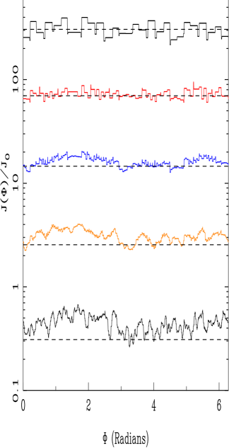
Figure 3.— The intensity as a function of angle in rings at a distance of $10,20,40,80,160\;h^{-1}{\rm Mpc}$ from a single quasar in the simulation density field. The straight lines show the uniform attentuation approximation. Normalized so that $J=1$ at $r=r_{\rm att}$ for uniform approximation.

The first thing that we notice is that the intensity decreases with distance, as expected. At a distance of 10 $\;h^{-1}{\rm Mpc}$, there are fluctuations present in the simulation results. These are largely due to the fact that as with the previous test we have rebinned the particles into cubic cells (a $256^{3}$ grid) and are plotting the mean intensity in each grid cell. As we move round the ring, the center of the closest cell to 10 $\;h^{-1}{\rm Mpc}$ can be up to $\sim 1\;h^{-1}{\rm Mpc}$ from it, which leads to expected fluctuations of order $\pm 20\%$. These fluctuations are solely an artefact of the binning used for the plot, and as expected diminish with distance.

As we reach the $40\;h^{-1}{\rm Mpc}$ ring, we see clear variations due to the anisotropy of the optical depths. At an angle $\Phi\sim 1.5\ {\rm Rad}$, there is an intensity $\sim 50\%$ higher than at $\Phi\sim 3\ {\rm Rad}$. The photons appear to have been travelling through a void and an overdense region respectively. The differences between the angles increase as we move farther out. We can also see that angles which were “in shadow” at small distances from the source keep the imprint at larger distances, as expected. The angular scale of the newly imprinted intensity fluctuations also appears to go down with distance, as should happen if they are associated with features with a fixed physical scale. At a distance of $160\;h^{-1}{\rm Mpc}$, the intensity fluctuations can be a factor of $\sim 2$. It can also be seen that at this distance for most of space there is a higher intensity than would be expected in the uniform attentuation approximation with $r_{\rm att}=111\;h^{-1}{\rm Mpc}$). There are however a few shadowed regions where photons had presumably not been moving through voids, and which are noticeably darker.

The situation with more sources present would of course be even more complex. One could argue that the angular variations would cancel out as each point in space can usually see more than one source at any given time. However, with sparse QSO sources, this number would not be large, and these sources would have their own shadows in front of them. We also note that it is likely that the $z=3$ situation, with the mean free path of photons being very large will be less sensitive to the difference between raytracing and the uniform attenuation approximation than higher redshifts. In order to test the difference between these two methods at $z=3$, we have carried out simulations using the uniform attentuation approximation and will present results for these later.

3.3. Lightcone effects

The light travel time across our $500\;h^{-1}{\rm Mpc}$ box is $6\times 10^{8}$ yrs at $z=3$. If the source lifetime is much less than this, then we may have to take this into account. For example, light will take 20 Myr to each a point $2\times 10^{7}$ light years away in space (we are using the Euclidean approximation). If the source has switched off by this time, then the radiation will remain as a light echo propagating through space (analogous to supernova light echos e.g., Crotts 1988). This will affect the ionization state of the IGM and the Ly$\alpha$ forest. If we were able to recieve information from all points in space at the same time, the light echos would appear as spherical shells centered on the position of each source, with a thickness equal to the source lifetime times the speed of light.

However, because we recieve information from the Universe at different times, the light echoes will not quite have this shape. Information from points behind a source will be from an earlier time than information that comes to us from in front of a source. Because of this the effect of the light echoes to an observer at a given time will not be spherically symmetric about the position of the source. We model these light cone effects as well as the finite lifetime of sources. In order to do this, we to calculate for each ray that we cast a minimum and maximum distance along it that the effect of its radiation will be present.

If these distances $r_{min}$ and $r_{max}$ are in comoving $\;h^{-1}{\rm Mpc}$ then we have the following for each source and ray:

$$r_{min}=A(1+z)\frac{ct_{off}}{1+{\hat{\underline{y}}}\cdot{\hat{\underline{r}}}}$$ (6)

and

$$r_{max}=A(1+z)\frac{ct_{on}}{1+{\hat{\underline{y}}}\cdot{\hat{\underline{r}}}}.$$ (7)

Here $t_{on}$ and $t_{off}$ are the times that the source switched on and off, respectively, in Myr, and $A=h/3.26$. The sources which are deemed to be on when the simulation is “observed” are on at the time the lightcone passes them. The $t=0$ point is set for each for each QSO to be the time of lightcone passage. The vector ${\hat{\underline{r}}}$ is the unit vector along the ray and ${\hat{\underline{y}}}$ is the unit vector along the line of sight direction (chosen here to be the $y$-axis).

We note here that we do not output the evolving density field on the lightcone, as we only make use of simulation density outputs at $z=3$. A more sophisticated treatment could do so (which would also mean sacrificing the periodic boundary conditions of the simulation volume). As long as we are only interested in predictions for one particular redshift, our approach is sufficient. Also, we will present results with and without radiation lightcone effects.

3.4. Quasar sources

We select the positions of luminous quasars in the dark matter simulations to be peaks in the density field. We then assign a luminosity to these peaks in order to reproduce the observed quasar luminosity function. Because the dark matter simulations have low mass resolution (particle masses for the d250 series are $1.6\times 10^{11}h^{-1}{\rm M_{\odot}}$), we use this approach rather than trying to identify halos, and we do not carry out a more sophisticated modelling of the quasar population (see e.g., Di Matteo et al 2003 for more detailed modelling of quasars in simulations).

In order to select peaks in the dark matter density field, we choose not to use a grid, but instead assign a density to each particle based on the distance to the 8th nearest neighbor. We then loop through the list of particles a second time, and if any particle has a higher density that its 8 nearest neighbors, then we define it to be a peak particle, with a peak height given by its density.

Each quasar is assigned to a peak particle. Varying the lifetime of quasar sources has potentially interesting effects, so that in this paper we will consider two different cases, source lifetime $t_{q}=10^{7}$ years, and $t_{q}=10^{8}$ years, chosen to bracket the expected range derived from other observations (e.g., Steidel et al. 2002). In each case, all quasars are chosen to have the same lifetime. We then compute the expected space density of quasars above a given magnitude limit using observational data (see below). From this, we compute number of quasars in the simulation active at one particular instant at $z=3$, $n_{now}$. We make the assumption that the number of quasars which were on at any time in the past is $n_{q}=n_{now}\times(t_{H}/t_{q})$, where $t_{H}$ is the Hubble time at $z=3$. The redshift difference between the edges of the box is $\delta_{z}=\pm 0.4$, so that our assumption effectively results in a non-evolving quasar population over that interval. We then select the highest $n_{q}$ peaks in the box and assign to each one a time that it switched on between 0 and $t_{H}$. Only the quasars which have $t_{on}<$ the light travel time across half the box are kept. In this model, each peak can have only host one active quasar phase during the time up to $z=3$.

Each quasar is then given a luminosity by drawing randomly from the B-band luminosity function used by HM96 and Sokasian et al. (2002):

$$\phi(L,z)=\frac{\phi_{*}}{L_{*}(z)}\left(\left[\frac{L}{L_{*}(z)}\right]^{\beta_{1}}+\left[\frac{L}{L_{*}(z)}\right]^{\beta_{2}}\right)^{-1}$$ (8)

Here $L_{*}(z)$ evolves with redshift so that:

$$L_{*}(z)=L_{*}(0)(1+z)^{\alpha-1}\exp[-z(z-2z_{*})/2\sigma^{2}_{*}]$$ (9)

The luminosity function parameters are $\beta_{1}=1.83,\beta_{2}=3.7,z_{*}=2.77,\sigma_{*}=0.91$ and $\log(\phi_{*}/{\rm Gpc}^{-3})=2.37$. This fitting formula (see Boyle, Shanks and Peterson, 1988, Pei 1995), ) is valid for an open universe with $h=0.5$, and as Sokasian et al. (2002) have done, we rescale the volume element and luminosity to that appropriate for our $\Lambda$CDM cosmology. Because we only directly simulate quasars with luminosity greater than $M_{b}=-25$, a portion of the background intensity may be contributed by fainter quasars. This will happen if the luminosity function above can be extrapolated to fainter magnitudes than observed, giving for example a $30\%$ higher intensity if we instead use $M_{b}<-22.5$.

We convert from a $B$-band luminosity to a source luminosity per Hz at 912Å assuming a quasar spectral index of $\nu=-1$. Below we will describe the intensity at $912$ Å that arises from the sources we do simulate and how we add an additional uniform radiation field (which we vary widely) to model other contributions (including those of fainter quasars).

3.4.1 Anisotropic radiation

The ionizing continuum radiation from quasars may not be emitted isotropically. Models of AGN unification (see e.g., the review by Urry and Padovani 1995) predict that an obscuring torus of material cuts down the emitted radiation to cones of opening angle $\sim 90^{\circ}$. We allow for this possibility by running models with and without this beaming of radiation (we use “beaming” in the rest of the paper as shorthand for this anisotropic emission of radiation, which should not be confused with relativistic beaming). In the case with beaming, we use an opening angle of $90^{\circ}$ and pick the orientation of the central axis randomly. This will mean that only $29\%$ of quasars are actually visible to an observer at one point. In order to match the observed number density, the actual space density of objects must therefore be increased.

3.4.2 Quasar clustering

A useful check of our simulated quasar sources is to compute their two-point correlation function. Because more massive host galaxies (or in our case higher peaks in the density field) are predicted to cluster more strongly (e.g., Bardeen et al. 1986), the correlation function has been proposed as a potential diagnostic of the quasar lifetime (longer lived quasars must be rarer and are therefore likely to be in more massive galaxies) by Martini and Weinberg (2001), and Haiman and Hui (2001). In our case, rough consistency with observed clustering is all we seek.

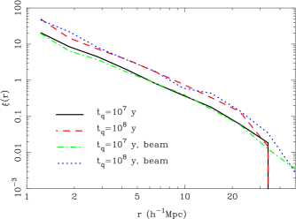
Figure 4.— Clustering of quasars measured in real space. We show the correlation function for two different quasar lifetimes and for isotropic and anisotropic emission.

In Figure 4 we show the correlation function $\xi(r)$ for quasars with two different lifetimes $t_{q}$ and with and without beaming. The quasars with $t_{q}=10^{7}$ yrs have a clustering amplitude $r_{0}=6.0\;h^{-1}{\rm Mpc}$ where $\xi(r)=(r/r_{0})^{\gamma}$ is the usual power law fit. The slope $\gamma=-2.0$, and is the same for the longer lived quasars, which have $r_{0}=8.5\;h^{-1}{\rm Mpc}$. There is no significant difference between the unbeamed and beamed quasars, although we might expect the beamed quasars to have a slightly lower clustering amplitude because of their higher space density. For comparison, $r_{0}=6.4^{+0.45}_{-0.44}$ for quasars from the 2dF QSO survey (Croom et al. 2002). This measurement is not however at the same redshift as our simulation, but for quasars chosen from the interval $z=0.3-2.9$, with a mean quasar redshift $\overline{z}=1.5$. The slope of the 2dF correlation function is also somewhat shallower $\gamma=-1.56$. If the clustering of observed quasars does not evolve from $z=3$ to $z=1.5$, this means that in the context of our simulations a lifetime close to $10^{7}$ years is favored. The 2dF quasars are however also fainter (by 2 absolute magnitudes in the mean) than our simulated sample (which more closely matches that of the Sloan Digital Sky Survey). This means that the 2dF quasars probably have lifetimes somewhat longer than $10^{7}$ years. The modelling uncertainties are considerable and our approach is fairly crude, so that this analysis can only give us a rough constraint on $t_{q}$.

3.5. Uniform background

In addition to quasars there are at least two other sources of ionizing radiation. One is recombination radiation, which HM96 compute should account for $30\%$ of the ionizing intensity at $z=3$. The other is galactic stars. The discovery of flux in the spectrum of Lyman Break Galaxies (LBGs) beyond the Lyman limit (Steidel et al. 2001) has led to some speculation that LBGs may contribute a substantial amount to the intensity (see e.g., Haenhelt et al. 2001, Hui, Zaldarriaga & Alexander 2002). Sokasian, Abel and Hernquist 2003, using radiative transfer calculations and simulations of structure formation find that in order to match the observed opacities of HeII and HI, the stellar contribution should contribute about equally with quasars at $z=3$.

Both of these sources of radiation will be distributed much more smoothly than quasars, having a significantly higher space density. The fluctuations at $z=3$ resulting from them will therefore be negligible. The radiation intensity flucutations resulting from LBGs at these redshifts have been explored by Adelberger et al. (2002), Croft et al. 2002, and Kollmaier et al. 2002 (the latter two using simulations of structure formation). In Croft et al. (1999), a simple analytic argument was made, using the results of Kovner and Rees (1989) to show that to a very good approximation we can treat the radiation coming from these numerous sources as uniform. At higher redshifts, as the opacity of the IGM increases, the number of sources within an attentuation volume decreases so that the fluctuations can become large, (see e.g., Meiksin and White 2003b). In our present simulations, we are concerned with $z=3$, and treat the additional radiation intensity from these sources as coming from a uniform background radiation field.

The mean intensity of this additional field is not observationally very well constrained. Guided by the results of Sokasian, Abel and Hernquist (2003), we choose, for our fiducial simulation to add a uniform intensity equal to that of the QSO contribution. We will also vary this quantity from a half to a factor of 64 times the QSO value in order to investigate its effects on clustering of the Ly$\alpha$ forest. We also directly compute the mean intensity (at $912$ Å ) contributed by the sources by first assigning the intensities seen by particles to a grid, and then volume averaging. We find $J=2.4\times 10^{-22}$, $1.7\times 10^{-22}$, and $1.6\times 10^{-22}$ for the d500, d250 and d125 simulations respectively (in units of ${\rm ergs^{-1}cm^{-2}Sr^{-1}Hz^{-1}}$.) We assume a spectral index for the uniform background identical to our assumed quasar spectral index of $\nu=-1$. This intensity can be compared to the value obtained using the proximity effect of $7.0^{+3.4}_{-4.4}\times 10^{-22}{\rm ergs^{-1}cm^{-2}Sr^{-1}Hz^{-1}}$ by Scott et al. (2000). The value of $J$ required to reproduce the mean opacity of HI in the Ly$\alpha$forest was estimated to be $2.3\times 10^{-22}$ by Rauch et al. 1997 (assuming an HM96 spectral shape; see also Weinberg et al. 1997). We note that for the smaller of our box sizes, many of the photons are not absorbed before they reach the maximum travel distance of half a box length. Because of the inverse square law, however, this only results in a small difference in the mean flux between the simulations, as mentioned above. We correct this difference by adding a small extra uniform component to the intensity for the d125 and d250 simulations to correct for the missing intensity, by comparing to the results of the d500 simulation.

3.6. The radiation field

In Figure 5 we plot the radiation field in slices through the simulation box, for one of the d250 realizations. This gives an idea of both the scale and morphology of the individual features, as well as the large scale structure in the field. The panels on the left side are for $t_{q}=10^{7}$ yrs and those on the right for $t_{q}=10^{8}$ yrs. The top panels do not include light cone effects, but the middle and bottom panels do, with the bottom panel being computed for anistotropically emitted radiation. In all cases, we have added our fiducial uniform background radiation with a level equal to the QSO contribution, as mentioned above.

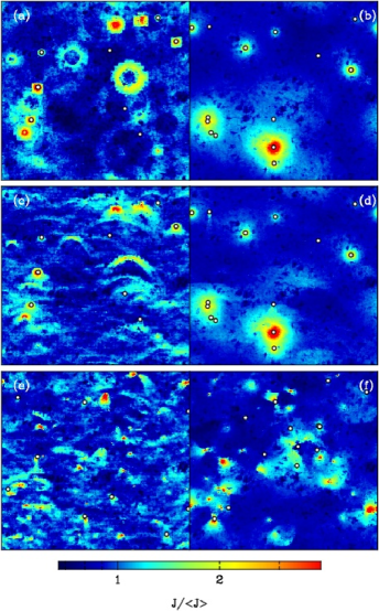
Figure 5.— The radiation intensity field ($J$, in units of the mean) in $25\;h^{-1}{\rm Mpc}$ thick slices through one of the d250 simulation volumes (box side length $250\;h^{-1}{\rm Mpc}$) at $z=3$. All panels show the same region of space, but with different assumptions/ approximations for the radiation emitted from quasars. The left panels are for quasars with a lifetime $t_{q}=10^{7}$ yrs and the right panels for $t_{q}=10^{8}$ yrs. Panels (a) and (b) are not output on the lightcone and have no quasar beaming. Panels (c) and (d) include lightcone effects (the observer’s line of sight is the y-axis) and isotropically emitted radiation. In panels (e) and (f), radiation is emitted from quasars in a cone of opening angle 90 degrees, and lightcone effects are included (see text). Quasars visible to an observer are shown as points.

For the top panels, without lightcone effects, the light echoes have the expected spherical shape. We show quasars visible (active) to an observer as points. It can be seen that for the shorter-lived quasars, as expected, much of the radiation has been emitted by quasars which are currently not active, whereas for $t_{q}=10^{8}$ yrs, many of the obvious high intensity radiation spots are centered on visible sources. Because of the coherence over long timescales of the radiation from the longer lived objects, the radiation field in the right panels appears smoother on small scales. We shall see below when we quantify the clustering in the Lya forest brought about by this inhomogeneous field that it is stronger on large scales.

In the middle row of Figure 5, the observer direction is towards the bottom of the plot, along the y-axis. Because of this, as explained in §3.3 above, the light echoes are not spheres. Quasars that are still on when the observation takes place have radiation around them which has propagated further in the direction of the observer than away. Quasars which have switched off recently enough that the inverse square law has not yet washed out their radiation are responsible for the bow shaped light echoes.

In the bottom row, the beamed quasars give the radiation field a different morphology. Roughly three times as many quasars are present as in the other panels, but only those for which the observer’s line of sight is within the radiation cone opening angle are shown as points. As in the other panels, most of the volume of space has an intensity about $80\%$ of the cosmic mean, with the region of space with intensity a factor of four or higher being very small indeed. The absorption seen in Ly$\alpha$ forest effectively samples the volume of the Universe reasonably fairly so that these small excursions of high intensity are unlikely to have much effect on Ly$\alpha$ forest clustering.

In order to make comparisons between the panels more quantitative, we have computed histograms of radiation intensities in cubical grid cells of side length $3\;h^{-1}{\rm Mpc}$. The results are shown in Figure 6. In this plot we also indlude our fiducial uniform background contribution as was done for the plots of slices through the radiation field. The $\%$ of pixels with $J$ twice the mean or more is $0.9-1.5\%$, and is lowest for $t_{q}=10^{7}$ years with lightcone effects and greatest for $t_{q}=10^{7}$ years without lightcone. The standard deviation of values is greatest (1.1) for the beamed quasars with $t_{q}=10^{8}$ yrs and least (0.58) for beamed $t_{q}=10^{7}$ years sources without lightcone effects. On the small scale of these cells, the difference between the quasars with different lifetimes is slight. The $t_{q}=10^{7}$ years objects have slightly larger fluctuations and a more skewed PDF, as might be expected from the complexity evident in the left panels of Figures 5. There is also even less change evident in the results when adding in lightcone effects and beaming.

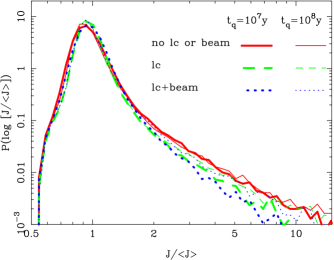
Figure 6.— The PDF of radiation intensities in units of the mean ($J/\langle J\rangle$) in the d250 simulation at $z=3$. We show results averaged spatially in cubes of side length $3\;h^{-1}{\rm Mpc}$. The y-axis gives the probability of finding a value of $\log J/\langle J\rangle$ between $\log J/\langle J\rangle$ and $\log J/\langle J\rangle+d\log J/\langle J\rangle$. The different line thicknesses show results for two differemt quasar lifetimes, and the different line styles results for either no beaming or light cone (lc) effects, light cone effects only, or both (as in Figure 5)

3.7. Lyman-alpha spectra

Now that we have an inhomogeneous radiation field, we create Ly$\alpha$ spectra that would be observed in quasar spectra whose sightlines pass through it. We assume that the hydrogen is in photoionization equilibrium with this radiation field (as mentioned previously, this is a good approximation if $t_{q}\lower 2.15277pt\hbox{$\;\buildrel>\over{\sim}\;$}10^{4}$ yrs). The neutral hydrogen density is inversely proportional to the photoionization rate $\Gamma$:

(10)

where

$$\Gamma=\int^{\infty}_{\nu_{HI}}d\nu\frac{4\pi J(\nu)}{h\nu}\sigma_{HI}(\nu)$$ (11)

The optical depth to absorption is given by

$$\tau_{Ly\alpha}=\frac{\pi e^{2}}{m_{e}c}f\lambda H^{-1}(z)n,$$ (12)

where $f=0.416$ is the Ly$\alpha$ oscillator strength, and $\lambda=1216$ Å (Gunn and Peterson 1965) The neutral density $n$ is inversely proportional to the photoionization rate for gas in photoionization equilibrium, and hence $\tau_{Ly\alpha}$ is inversely proportional to the intensity of the radiation field. With high resolution simulations which resolve the relevant length and mass scales (see e.g., Bryan et al. 1999 ), the optical depth can be calculated directly for each point in the spectrum. The optical depths are then convolved with the line-of-sight peculiar velocity field and thermal velocities to produce a redshift space spectrum (see e.g., Hernquist et al. 1996).

Dark matter only simulations have also been used to make spectra (e.g., Petitjean et al. 1995, Gnedin & Hui 1998, Croft et al. 1998, Meiksin and White 2001), making use of the fact that dark matter traces the gas density well on scales larger than the Jean’s scale. In the present case, because we are are interested in large-scale clustering of the Ly$\alpha$ forest, we have too low resolution to make realistic spectra directly, even using the dark matter as a proxy for baryons. Instead, we again appeal to the high resolution hydro simulation of §2.2. Our approach involves finding the flux in relatively large pixels which are associated with a given density of dark matter.

First we find the redshift space dark matter density and the ionizing radiation intensity in the dark matter simulations in cubes lying along sightlines through the box. The cubes are chosen to be relatively large (diameter $3/256$ of the box size, which is $3\;h^{-1}{\rm Mpc}$ for the d250 runs). We compute redshift space quantities, shifting the particle positions along the sightline axis by adding their peculiar velocities to their Hubble velocities. As $J$ values are associated with each particle, we compute the $J$ field in each cell from the particles which fall into the cell in redshift space.

In order to make use of the high resolution hydro simulation, we then randomly place within it cubical cells of the same size used for the dark matter simulations and compute the redshift space dark matter density in those cells. We next compute 1500 high resolution Ly$\alpha$ spectra which pass through the centers of the cells The spectra are computed from the neutral hydrogen density by integrating through the SPH kernels of the particles, and then convolving with the line of sight velocity field, in the usual manner (see e.g., Hernquist et al. 1996, or Croft et al. 2002 for the same simulation). The intensity of the ionizing background can be adjusted after the simulation was run, and we do so to reproduce a mean Ly$\alpha$ forest flux of $\langle F\rangle=0.64$ (from Press, Rybicki and Schneider 1993). We then average the unabsorbed flux $\langle F\rangle=\langle e^{-\tau}>$ inside each pixel that lies onspectra passing through the center of each cell, so that we have the F value which would be observed for a large pixel of size 32, 65, and 130 ${\rm\;km\;s^{-1}}$ for the d125, d250 and d500 simulations respectively (the cell size in redshift space). We make spectra several times over, each time varying the intensity of the ionizing background, from 100 to 0.01 times our fiducial intensity, in 20 log spaced bins.

Given this information, we now have, for a given overdensity of dark matter and radiation intensity at 912 Å a distribution of possible values for the Ly$\alpha$ forest flux in a large pixel. We use this to map our large low resolution dark matter skewers into spectra. We try two different methods for doing this. The first method (which we shall use for the rest of the paper) is to pick a random F value from the set of pixels with the correct dark matter density and J value. The second is to assign to the pixel the mean value of $\langle F\rangle$ for all pixels with the correct correct dark matter density and J value. For all the statistics we compute in the rest of the paper there is negligible difference between the two methods.

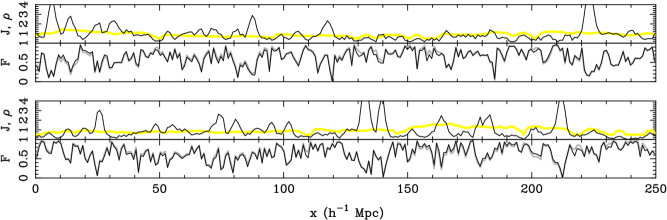
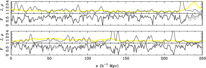
Figure 7.— Two randomly chosen line of sight density (dark line) and radiation (light line) fields (in units of the mean) for the no lightcone $t_{q}=10^{7}$ yr quasars (top 2 panels) and for the no lightcone $t_{q}=10^{8}$ yr quasars (bottom 2 panels). Under the radiation and density we show spectra made from these sightlines with a uniform radiation field (light line) and non uniform (dark line).

In Figure 7 we show the Ly$\alpha$ spectra that result from two randomly chosen sightlines through one of the d250 simulations. We also show the dark matter density and radiation intensity along the same sightlines, both in units of the cosmic mean. Each sightline is shown twice, for two values of the quasar lifetime ($t_{q}=10^{7}$ yrs and $t_{q}=10^{8}$ yrs) and results are without lightcone effects. The density field (smoothed with a $3\;h^{-1}{\rm Mpc}$ filter) obviously fluctuates more than the J field, showing that the density is the source of most structure. There is only one moderately large excursion in $J$ above the mean for the first sightline (for $t_{q}=10^{8}$ yrs) where a foreground quasar was present. The difference between the two values of $t_{q}$ is not easy to see in the radiation field, but it seems plausible that there are larger scale $J$ fluctuations for longer $t_{q}$. The Ly$\alpha$ forest spectra are shown next to spectra that result from a uniform $J$. The difference is very small, with a maximum difference in $F$ of 0.17 between the two. The effect of gentle long wavelength fluctuations in $J$ can be seen, particularly in the bottom-most panel.

4. The Lyman-alpha power spectrum

Having created an inhomogenous radiation field from a population of quasar sources and Ly$\alpha$ forest spectra running through it, we now turn to Ly$\alpha$ forest observables. In this section we measure the large-scale clustering of our Ly$\alpha$ forest spectra using the power spectrum, and investigate its dependence on the assumptions we have made regarding quasar lifetimes, radiation contributed by other sources and inclusion of lightcone effects and beaming. The power spectrum of the density distribution in the Universe is a useful probe of cosmology, and the relatively simple physics relating Ly$\alpha$ forest flux and density has made it possible to use Ly$\alpha$ forest data for this purpose (see e.g. Croft et al. 1998, Hui 1999, McDonald et al. 2000). Observational constraints on P(k) have been made by McDonald et al. (2000), Zaldarriaga, Hui & Tegmark (2001), Gnedin & Hamilton (2002) and Croft et al. (2002), amongst others. It is of particular interest to see if radiation fluctuations can disrupt the relation between density and Ly$\alpha$ forest flux enough to affect cosmological measurements.

We compute the one-dimensional power spectrum of the Ly$\alpha$ forest spectra by first calculating a mean flux contrast field:

$$\delta_{F}(\lambda)\equiv F(\lambda)/\langle F\rangle-1$$ (13)

The power spectrum is then given from the variance of Fourier modes with a given $k$, so that

$$\delta(k)=\frac{1}{2\pi}\int\delta(x)e^{-ikx}dx,$$ (14)

and the dimensionless (1-dimensional) power spectrum,

$$\Delta_{F}^{2}(k)=\frac{k}{\pi}\langle\delta(k)^{2}\rangle.$$ (15)

In Figure 8, we show some simulation results, which we shall describe below. We also show observational results for $\Delta^{2}_{F}(k)$ from Croft et al. (2002). These were computed from pixels in spectra which were within $\delta_{z}=^{+0.2}_{-0.1}$ of $z=3$. The length scales in ${\rm\;km\;s^{-1}}$ have been converted to comoving $(h^{-1}Mpc)^{-1}$ assuming our $\Lambda$ cosmology. The half-wavelength $\pi/k$ of the largest scale plotted is $14\;h^{-1}{\rm Mpc}$. This measurement was made from a subsample of the Croft et al. dataset which contained 53 quasar spectra. Datasets two or three orders magnitude larger are forthcoming from the Sloan Digital Sky Survey (see e.g., Hui et al. 2003, Seljak et al. 2003), and it will be possible to measure $\Delta^{2}_{F}(k)$ on much larger scales with them (modulo other uncertanties such as continuum fitting).

4.1. Convergence tests

With our Monte-Carlo method for raytracing, shot noise in the number of photon packets could result in unphysical fluctuations in the radiation field if not enough are used. In Figure 8, we compute $\Delta^{2}_{\rm F}(k)$ using 1000 Ly$\alpha$ spectra taken from a single realization of a d500 simulation. In the bottom panel, $\Delta^{2}_{\rm F}(k)$ itself is plotted, whereas in the top panel we show the ratio of $\Delta^{2}_{\rm F}(k)$ for spectra computed with a uniform background which we call

$$\delta_{u}=^{\rm uniform}\Delta^{2}_{\rm F}(k)/\Delta^{2}_{\rm F}(k).$$ (16)

We compute these quantities after using a variable number of photon packets to generated the radiation field, from $10^{6}$ to $64\times 10^{6}$. The results appear to have converged after $16\times 10^{6}$ photon packets. For the rest of our calculations, we shall use $32\times 10^{6}$.

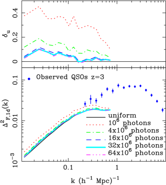
Figure 8.— Convergence test for the number of photon packets to be used in raytracing. We show the power spectrum of the Ly$\alpha$ forest flux $\Delta^{2}_{\rm F}(k)$ in the d500 simulation (no light cone effects or beaming), for different numbers of photon packets. The top panel shows the fractional difference in $\Delta^{2}_{\rm F}(k)$ between the raytraced simulation and one using a uniform radiation field (Equation 16).

As we have run simulations with three different box sizes, we are also able to check convergence of $\Delta^{2}_{\rm F}(k)$ with spatial resolution and particle mass. For the rest of the figures in this paper, we use 1000 spectra from each simulation realization and average over 5 realizations. In Figure 9 we show $\Delta^{2}_{\rm F}(k)$ measured from the d125, d250 and d500 simulations (all outputs including lightcone effects, but no beaming). The bottom panel shows results for a uniform radiation field, and the top two the ratio $\delta_{u}$ for the two different lifetimes. In the bottom panel we can see that the absolute value of $\Delta^{2}_{\rm F}(k)$ has converged well over the range of scales that are resolved by all 3 simulations ($\sim 0.05-0.15\;h\;{\rm Mpc}^{-1}$). The d125 simulations are of high enough resolution that they can be compared with one or two of the largest scale observational points, and are reasonably consistent.

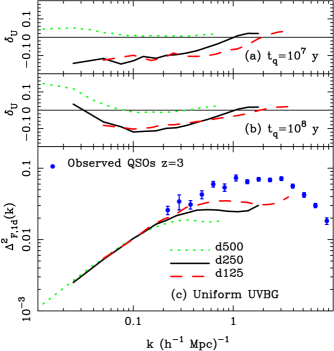
Figure 9.— Convergence test for the box size, force resolution and particle mass. We show the power spectrum of the Ly$\alpha$ forest flux $\Delta^{2}_{\rm F}(k)$ averaged over all realizations for the three sets of simulations with different box sizes and particle masses. In this case output was on the lightcone, but the radiation output of quasars was set to be isotropic. The top panel shows the fractional difference (Eqn. 16) in $\Delta^{2}_{\rm F}(k)$ between the raytraced simulation and that using a uniform radiation field.

In the top two panels of Figure 9, we can see that the power spectra relative to that with a uniform $J$ only converge when we reach the d250 resolution. The d500 $\delta_{u}$ is actually slightly greater than 1, whereas the converged result shows that the $J$ fluctuations suppress the Ly$\alpha$ power spectrum (as seen by Meiksin and White 2003b at higher redshifts $z>4$). The power spectrum suppression is about $10-12\%$ on scales $k\sim 0.1\;h\;{\rm Mpc}^{-1}$. Both values of $t_{q}$ give similar results on these scales, whereas on larger scales $k\sim 0.05\;h\;{\rm Mpc}^{-1}$, $\delta_{u}$ for the long lived quasars is becoming positive again. This corresponds to physical scales of half-wavelength $\sim 100\;h^{-1}{\rm Mpc}$, or close to the distance light can travel in $10^{8}yrs$. For scales $k\lower 2.15277pt\hbox{$\;\buildrel>\over{\sim}\;$}1\;h\;{\rm Mpc}^{-1}$, $\delta_{u}$ becomes close to zero, at least for the large value of $t_{q}$, indicating that fluctuations due to the inhomogeneous radiation field are unlikely to affect $\Delta^{2}_{\rm F}(k)$ on presently observed length scales at more that the $1-2\%$ level. For the results with $t_{q}=10^{7}$, the results have not converged quite as well on the smallest scales, indicating that there is room for a small amount of excess power. However, this regime of lengthscales has been probed (at $z=4$) by Gnedin and Hamilton (2002), and by Meiksin and White (2003b), who find minimal effects.

4.2. Lightcone, beaming and uniform background effects on the Ly$\alpha$ power spectrum

Given that the d250 simulations have converged for most of the range of length scales we are interested in, we now examine the effect of including output on the lightcone and anisotropically emitted radiation in these runs. In Figure 10 we show $\Delta^{2}_{\rm F}(k)$ for outputs with and without these effects, for both values of $t_{q}$. We find that including lightcone effects increases the amplitude of the radiation fluctuations, making suppression of the Ly$\alpha$ power spectrum stronger by roughly a factor of 2. The presence of beamed radiation makes little difference, however, which is somewhat suprising. It seems as though the smoothing effect on the radiation field from having more sources per unit volume has been cancelled out by the fluctuations due to the limited beaming angle around each source. Even though the effect of beaming on the one dimensional Ly$\alpha$ forest statistic is minimal, the radiation field itself does look dramatically different, as one can see by comparing panels (e) and (f) of Figure 5.

The results of an additional test are shown in Figure 10. As mentioned in §3.2 we have also computed the radiation field assuming the uniform attentuation approximation, where there is no shadowing of light and photons travel isotropically from each source. We have used an attenuation length of $111\;h^{-1}{\rm Mpc}$ appropriate for a uniform medium. For the lightcone case with $t_{q}=10^{7}$ y, we plot the results in Figure 10, where they can be compared with the full treatment. We find that the differences are quite small, with $\delta_{u}$ being essentially identical for $k>0.05\;h\;{\rm Mpc}^{-1}$ and only different by $20\%$ on the largest scales. From this we can conclude, that the effect of shadowing in the largely optically thin Universe at $z=3$ is minimal. For this statistic at least, the inclusion of lightcone effects is more important.

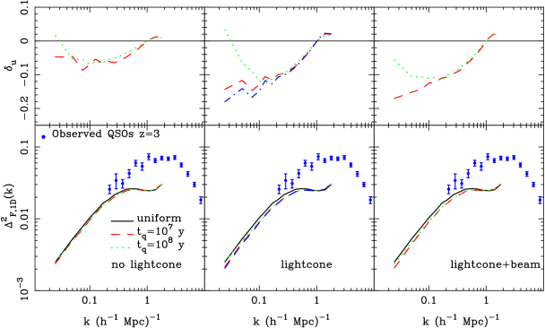
Figure 10.— The effect of output on the lightcone and anisotropic QSO radiation on the power spectrum of the Ly$\alpha$ forest flux $\Delta^{2}_{\rm F}(k)$. We show results for a uniform radiation field, and raytraced field with two quasar lifetimes. In the middle panels, the dot-dashed line is the result for the uniform attentuation approximation (see text). The top panels show the fractional difference in $\Delta^{2}_{\rm F}(k)$ between the raytraced simulations and those using a uniform radiation field.

As explained previously, there will be a much more uniform component to the radiation field, originating from recombination radiation and stellar sources in galaxies. We expect that the mean intensity contributed in this way will be approximately equal to that from quasars (Sokasian et al. 2003). In Figure 11, we explore the effect on $\Delta^{2}_{\rm F}(k)$ of adding an an extra uniform contribution. We vary this uniform background to be from 0.5 to 8 times that of amount from quasars, and find that the suppression of $\Delta^{2}_{\rm F}(k)$ relative to a uniform $J$ field goes down as the uniform background level is raised, as expected. Doubling the uniform field compared to our fiducial level changes the maximum supression from $12\%$ to $8\%$ for $t_{q}=10^{8}$. With a uniform field larger than our fiducial one, there is no boost in $\Delta^{2}_{\rm F}(k)$ on the largest scales either. We have also tried reducing our fiducial uniform background by a factor of 2, and results are also shown in Figure 11. In this case, the suppression measured by $\delta_{u}$ is stronger (about $18\%$ maximum suppression).

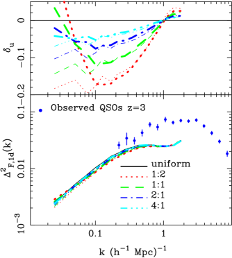
Figure 11.— The effect of adding a uniform component to the raytraced radiation field on the power spectrum of the Ly$\alpha$ forest flux $\Delta^{2}_{\rm F}(k)$. The ratio of uniform component to component coming from QSO sources is shown in the legend (e.g., 2:1 means that the contribution to the spatially averaged intensity from a uniform field is twice that from the sources). We show results for the d250 simulations, with output on the lightcone, and for $t_{q}=10^{7}$ yrs (thin lines), and $t_{q}=10^{8}$ yrs (thick lines) The top panel shows the fractional difference in $\Delta^{2}_{\rm F}(k)$ between the raytraced simulations and those using a totally uniform radiation field.

It is interesting to examine the potential effects of this suppression of $\Delta^{2}_{\rm F}(k)$ on work which seeks to constrain the matter power spectrum from Ly$\alpha$ forest measurements. Data from the Sloan Digital Sky Survey will probe larger scales than those in the analyses by Croft et al. (2002), for example. A uniform suppression of $\Delta^{2}_{\rm F}(k)$ by $10\%$ at redshifts close to these would translate to a reduction in the inferred amplitude of mass fluctuations ($\propto\sigma_{8}$) of $\sim 7\%$ (Croft et al. 2002). The fact that $\delta_{u}$ changes with scale will slightly alter the shape of the inferred mass power spectrum. We will return to this in our discussion in §6.

5. Foreground proximity effect

We have seen that the effect of radiation fluctuations on the overall clustering of the Ly$\alpha$ forest at $z=3$ is likely to be small. Close to QSO sources, however, the locally produced radiation can overwhelm the background and produce much stronger effects. The effect of a QSO’s radiation on its own Ly$\alpha$ forest, known as the proximity effect, has been extensively studied, first by Bajtlik, Duncan and Ostriker (1988). Because the ionizing radiation studied in such a case is that along the line of sight to the quasar, as long as the quasar source turned on within the equilibration time ($\sim 10^{4}$) years of being observed, the Ly$\alpha$ forest will respond and the effect can be seen. The relative suppression of absorption (quantified by the number of Ly$\alpha$ lines) caused by the ionizing radiation close to the quasar has been used to constrain the overall intensity of the background field by Cooke, Espey & Carswell (1997), Scott et al. (2000), among others.

The effect of radiation from a QSO on the Ly$\alpha$ forest of other quasars is known as the foreground or transverse proximity effect. Because the light travel time to a sightline 10 $\;h^{-1}{\rm Mpc}$ away in the transverse direction is $\sim 10^{7}$ y, the presence or absence of an effect can be used to constrain the lifetime of the QSO. The use of the foreground proximity effect to do this has been explored recently by Schirber, Miralda-Escudé, & McDonald (2003), using data from the Sloan Digital Sky Survey Early data release. These authors found no evidence of an effect, something we shall return to later. The foreground effect has also been examined theoretically by e.g., Kovner & Rees (1989), and possible detections have been reported by Dobrzycki & Bechtold (1991), Jakobsen et al. (2003), and limits by Liske & Williger (2001).

In this paper, we will not examine the foreground proximity effect around individual sources but instead the averaged Ly$\alpha$ forest flux around all quasars, $\langle F\rangle(r)$. The mean Ly$\alpha$ forest flux as a function of distance from Lyman Break Galaxies was measured by Adelberger et al. (2003), and from simulations by Croft et al. (2002), and Kollmaier et al. (2002), and Bruscoli et al. (2003). We will carry out the same measurement for QSOs, making predictions from our simulations and an observational measurement from SDSS data. We will not be measuring the effect of each quasar on its own Ly$\alpha$ forest, as this requires accurate modelling of the continuum close to the quasar, including its Ly$\alpha$ line emission, and is left for future work.

5.1. SDSS First Data Release

Our observational determination of $\langle F\rangle(r)$ is made using the first data release of the Sloan Digital Sky Survey (Abazajian et al. 2003). We have taken all spectra for which some part of the Ly$\alpha$ forest region is available above $z=2.2$ which includes 1920 spectra. The mean redshift of all Ly$\alpha$ forest pixels in this region is $z=2.81$, and the mean S/N is 5.7. We do not fit a continuum to these spectra but remove the continuum dependence by instead first smoothing them with a Gaussian filter of width $\sigma=50$ ÅẆe do not try to determine the absolute mean flux level of the spectra, but assign a value based on the work of Press, Rybicki and Schneider (1993, PRS), which is largely consistent with the mean flux measured from SDSS spectra by Bernardi et al. (2002). To do this, the flux value of a pixel at redshift $z$ is given by

$$F_{z}=\frac{S_{z}}{C_{z}}\times PRS_{z},$$ (17)

where $S_{z}$ is the spectrum, $C_{z}$ is the value of the smoothed spectrum and $PRS_{z}$ is the value of the mean flux from the PRS data at redshift $z$. We note that because our simulated spectra were normalized to have the PRS mean flux we are therefore consistent. Continuum fitting is a difficult procedure and uncertainties in the observationally determined values are still large. For example, it is very possible that the PRS determination of the mean flux is too low (see e.g., Seljak, McDonald & Makarov 2003) . Although this is an important question which must be resolved, in the case of the present paper, as long as the simulations and observations are normalized using the same values, these uncertainties will not affect our comparisons.

As mentioned above, the region close to the Ly$\alpha$ emission line must be treated with special care if it is to be used. In the current work, we are conservative and instead only use Ly$\alpha$ pixels with rest frame wavelength between $1060$ Å and $1160$ ÅȦlso, as we are interested in the mean flux of pixels averaged around QSOs, only pixels which fall close to QSOs will actually be used. We convert redshifts and angular coordinates of all pixels into 3 dimensional cartesian comoving coordinates, assuming a flat cosmology with $\Omega_{M}=0.3$ and $\Omega_{\Lambda}=0.7$. After doing this, only pixels within 40 $\;h^{-1}{\rm Mpc}$ of a QSO are kept. This cuts down the number of contributing QSOs to 325. The mean $z$ of these pixels is $z=2.6$, and the mean absolute QSO magnitude in the SDSS $G$ band is $-27.2$ (our simulated quasars have a similar mean $G$ magnitude of $-27.0$, again assuming a spectral index of $\nu=-1$ to transform from $B$ to $G$ magnitude). Because we are interested in comparing to our simulation results at $z=3$, we have changed the mean value of the absorption in Equation 17 to $PRS_{z+0.4}$. By doing this, we are assuming that the effect of changing mean flux between $z=2.6$ and $z=3.0$ is more important to $\langle F\rangle(r)$ than the change in the density field around QSOs. In order to test this, we have tried setting the lower bound on pixel redshifts to $z=2.5$, which gives a mean pixel redshift of $z=3.0$, and calculating $\langle F\rangle(r)$ without using any offset in Equation 17. We find results that are much noiser, but consistent within the errors. With future releases of SDSS data it will be possible to measure $\langle F\rangle(r)$ of a larger sample of QSOs at many redshifts.

In Figure 12, we show $\langle F\rangle(r)$ for the SDSS QSO sample, compared to the results for Lyman Break Galaxies of Adelberger et al. (2002). The Adelberger et al. points show increased absorption with respect to the mean over the range from $\sim 2-10\;h^{-1}{\rm Mpc}$ (comoving) from galaxies. On smaller scales, there is evidence (at the $2-3\sigma$) level for decreased absorption, or a proximity effect. What the cause of this lack of absorption close to galaxies might be was considered extensively by Adelberger et al. (see also Croft et al. 2002 and Kollmeier et al. 2002). It was concluded that a radiation proximity effect could not be the answer because the ratio of the ionizing background radiation to the galaxies own is too high, even at distances of $\sim 1\;h^{-1}{\rm Mpc}$. Galactic winds blowing holes in the IGM seem to be a possibility, although hydrodynamic simulations of winds in a cosmological context do not exhibit the required strong modulation of the Ly$\alpha$ forest flux (see Theuns et al. 2002, Viel et al. 2003). Measuring the redshift of the galaxy to enough precision that any signal at these small scales is not washed out by position errors is extremely difficult, so that Adelberger et al. caution that this proximity effect result is tentative at best.

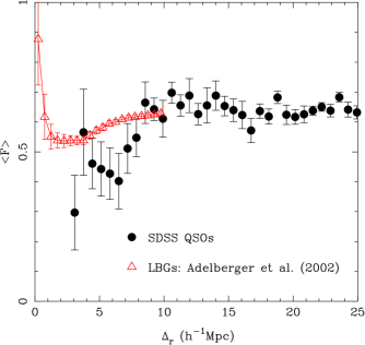
Figure 12.— The mean Ly$\alpha$ forest flux $\langle F\rangle$ at $z=3$ averaged around quasars in the SDSS First Data Release as a function of quasar-pixel distance (round points). Also shown are results at $z=3$ for Lyman-break galaxies (Adelberger et al. 2002).

The space density of the LBGs in present samples is $1.5\times 10^{-2}h^{3}{\rm Mpc^{-3}}$ (for a magnitude limit of 25.5, see e.g., Adelberger et al. 2002). This is a factor $\sim 1000$ times higher than that of the SDSS QSOs we have used to compute the solid points in Figure 12. With $\langle F\rangle(r)$ for the QSOs, there is also substantially more absorption than the mean, again up to distances of around $\sim 10\;h^{-1}{\rm Mpc}$. This excess absorption is to be expected if QSOs sample dense environments, and if the effect of this excess absorption is not outweighed by the effect of ionizing radiation from the QSO. We can see that there appears to be no direct evidence of ionizing radiation, no foreground proximity effect. In the next subsection, we shall explore what we expect from our models and make a comparison. For now, it is obvious that the excess absorption is substantially greater than around LBGs at $z=3$, so that the QSOs appear to be located in much denser environments and possibly more massive dark matter halos. There is no information on scales below $3\;h^{-1}{\rm Mpc}$ due to the sparsness of the QSO sample. Within $10\;h^{-1}{\rm Mpc}$, 22 QSOs contribute at least 1 pixel to the measurement of $\langle F\rangle(r)$, but for the 3 points with $r<=5\;h^{-1}{\rm Mpc}$, only 5 contribute. We note that these numbers are also equal to the numbers of pairs of QSOs with these separations. This is because our restricted wavelength range means that only the lower redshift QSO in each pair is used as a center when we average pixels at a given distance from it. The mean SDSS G magnitude of the QSOs in both these cases is $-27.2$. The error bars in Figure 12 have been computed using a jackknife estimator (Bradley 1982) with a number of subsamples equal to the number of quasars in each bin.

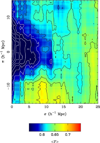
Figure 13.— The mean Ly$\alpha$ forest flux $\langle F\rangle$ at $z=3$ averaged around quasars in the SDSS first data release as a function of quasar-pixel distance across the line of sight ($\sigma$) and along the line of sight ($\pi$). In order to reduce the effects of noise, the data was smoothed with a Gaussian filter with standard deviation $5\;h^{-1}{\rm Mpc}$.

The data shown in Figure 12 is a radial average of the mean flux around QSOs. However, there are many reasons to suppose that the absorption could show a different dependence on QSO-pixel distance transverse to (often referred to as $\sigma$) and along the line of sight ($\pi$). We will investigate these in more detail when we consider models below. For now, we will note that any ionizing radiation propagating in the direction away from the observer (+ve $\pi$) will have less time to reach a pixel at a given $|r|$ than if it were moving in the opposite direction. This as we have already noted is the cause of the lightcone effects seen in §3.3, and will lead to the mean flux $\langle F\rangle$ being possibly asymmetric about the $\pi=0$ axis. An additional possibility is that beamed radiation will cause a proximity effect only at small angles to the $\pi$ axis. In order to investigate these possibilities we have plotted $\langle F\rangle(\sigma,\pi)$ for our SDSS sample in Figure 13. In order to make the contours more visible, we have smoothed the plot with a Gaussian filter with standard deviation ${}_{e}\sigma 5\;h^{-1}{\rm Mpc}$. The excess absorption compared to the mean is clearly visible close to the position of the QSO. There is also no obvious sign of asymmetry about the $\pi=0$ axis. In order to quantify this, we have computed jackknife errors for $\langle F\rangle(\sigma,\pi)$ (in $5\times 5\;h^{-1}{\rm Mpc}$) bins. We have then computed the sum

$$\chi^{2}=\sum_{i,j}\langle F\rangle(\sigma,\pi)-\langle F\rangle(\sigma,-\pi)/_{e}\sigma^{2}$$ (18)

where ${}_{e}\sigma^{2}$ is ${}_{e}\sigma_{i,j}^{2}+_{e}\sigma_{i,-j}^{2}$ is the error. We find $\chi^{2}=60.6$ for 64 bins, so that within the statistical uncertainty there is no evidence for any asymmetry. Figure 13 does not show very marked elongation of the contours along the $\pi$ axis either, which could be a sign that the QSOs are not found in large virialized systems.

5.2. Simulation results

We have seen that the SDSS QSOs show no signs of decreasing the absorption in other lines of sight passing close by. The situation is rather different in our simulations, as we see in Figure 14. Here we have computed $\langle F\rangle(r)$ for all three sets of simulations, the d500, d250 and d125, and for the two different quasar lifetimes. In the top panel, we show results including an inhomogeneous radiation field (with lightcone effects, but no beaming). It is clear that there is a slight proximity effect close to the QSOs, and that there is not much difference between the different simulations. As with the convergence test of $\Delta^{2}_{\rm F}(k)$ (Figure 9), the d250 and d125 runs appear to be somewhat closer together than the d500 results. The simulation curves differ radically from the observational results on scales $r<8\;h^{-1}{\rm Mpc}$. This is rather surprising, as based the simulations, we would expect to see some sign of the radiation field in the real data, but there appears to be none.

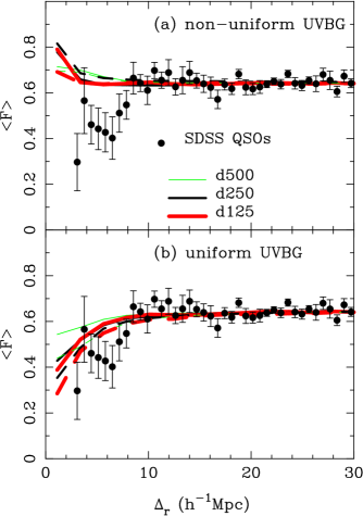
Figure 14.— Effect of resolution and box size on the Ly$\alpha$ forest flux averaged around simulated quasars as a function of quasar pixel distance. We show results for all three simulation sets, in each case averaging over all realizations. The solid lines are for quasar lifetime $t_{q}=10^{7}$ y and the dashed lines for $t_{q}=10^{8}$ y (output is on the lightcone but there is no beaming of radiation). The solid points are the observational data computed from the Sloan Digital Sky Survey First Data Release.

Without QSOs acting as sources, however, we do find a closer match. In the bottom panel of Figure 14, we show the $\langle F\rangle(r)$ curves which result in our simulations if we assume a homogeneous radiation field. The increased absorption resulting from QSOs being found in dense environments is then seen, and it is clear that the almost flat nature of $\langle F\rangle(r)$ in the top panel is the result of this increased absorption being largely cancelled out by the QSO radiation flux. In the uniform radiation field case, the QSOs with $t_{q}=10^{8}$ have marginally more absorption on scales $r<12\;h^{-1}{\rm Mpc}$ from the QSO (this quantity has converged well with resolution for the d125 and d250 simulations). If we compare with observations, though, even these rare quasars do not have enough absorption to match well.

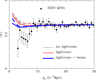
Figure 15.— Effect of anisotropic radiation and output on the light cone on the Ly$\alpha$ forest flux averaged around simulated quasars as a function of quasar pixel distance. We show results for the d250 simulation set only, averaging over all realization. The solid lines are for quasar lifetime $t_{q}=10^{7}$ y and the dashed lines for $t_{q}=10^{8}$ y. The solid points are the observational data computed from the Sloan Digital Sky Survey First Data Release.

With the simulations, we can test the effect of turning off output on the lightcone. This is shown in Figure 15. We might not expect this to have much effect on this statistic because the distances of interest correspond to relatively short light travel times. From the plot we can see that the effect of ignoring lightcone effects is neglgible for $t_{q}=10^{8}$ yrs, and not important even for $t_{q}=10^{7}$ yrs. Of course if we were to condider $t_{q}$ of the same order or less as the light travel time across the proximity effect region, then these effects would become substantial. Schirber et al. (2003) have studied the proximity effect as a probe, across sightlines and conclude that it can yield interesting constraints on $t_{q}$. They find that a $t_{q}$ of the order of $10^{6}$ years could be part of the explanation for the lack of proximity effect seen by them in a sample of SDSS data. We will return to this in §6.

If the radiation emission is highly anisotropic, then of course we would not expect to see regions off axis being illuminated by the QSO. The radially averaged statistic $\langle F\rangle(r)$ should therefore show less of a proximity effect, as we are averaging with some pixels at angles which see only the background radiation. Figure 15 shows that this is indeed the case, although the beaming angle we have chosen (opening angle of cone=$90\deg$) is too large to have much of an effect, and $\langle F\rangle(r)$ in the simulations is still too high on small scales compared to the observations. Our opening angle was chosen based on what is considered theoretically likely (Urry & Padovani 1995). The fact that an opening angle much smaller (by a factor of 3 or more) would be necessary in order to even approach what is seen in the observations makes it likely that anisotropically emitted raditiaion is not the sole cause of the discrepancy between our simulations and observations.

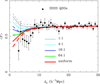
Figure 16.— The effect of adding a uniform component to the raytraced radiation field on the Ly$\alpha$ forest flux averaged around simulated quasars as a function of quasar-pixel distance. The ratio of uniform component to component coming from QSO sources is shown in the legend (e.g., 16:1 means that the contribution to the spatially averaged intensity from a uniform field is 16 times that from the sources). We show results for the d250 simulation set only. averaging over all realizations. The solid lines are for quasar lifetime $t_{q}=10^{7}$ y and the dashed lines for $t_{q}=10^{8}$ y. The solid points are the observational data computed from the Sloan Digital Sky Survey First Data Release.

One way of reducing the relative effect of the radiation from an individual quasar is by increasing the strength of the background field. Of course, for the regular proximity effect, this has long been used as a measure of the background field itself, given a known flux of radiation from the quasar. Because of these measurementsscott and other considerations, the amount of background radiation not coming from QSOs is not a free parameter, but is constrained to be about equal to that from the sum total of QSO radiation (e.g., Sokasian et al. 2003). The observational errors are large (e.g., for Scott et al. 2000, the allowed intensity can vary by $+50\%,-60\%$ within $1\sigma$). Nevertheless, it is instructive to vary the intensity of our additional homogeneous radiation field much more than this in order to investigate how much it can change the foreground proximity effect. In Figure 16, we show the $\langle F\rangle(r)$ which results when the background field is changed from our fiducial value (equal to the QSO contribution) to 64 times that value. As expected, increasing the background reduces the effect of the local radiation. However, even with a background 16 times too high, there is still some evidence of a proximity effect, and the simulations are far from the observational points. Even if QSOs are responsible for a tiny fraction of the intensity of the ionzing radiation field at $z=3$ (which does not seem likely), this will not solve our discrepancy.

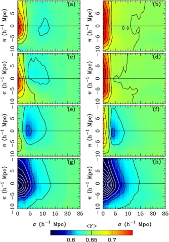
Figure 17.— The mean Ly$\alpha$ forest flux $\langle F\rangle$ as a function of distance across ($\sigma$) and along ($\pi$) the line of sight from simmulated quasars. The left panels are for quasars with a lifetime $t_{q}=10^{7}$ yrs and the right panels for $t_{q}=10^{8}$ yrs. Panels (a) and (b) are not output on the lightcone and have no quasar beaming. Panels (c) and (d) include lightcone effects (the observer’s line of sight is the y-axis) and isotropically emitted radiation. In panels (e) and (f), radiation is emitted from quasars in a cone of opening angle 90 degrees, and lightcone effects are included (see text). In panels (g) and (h) the radiation field is uniform.

Additional information is available to us if we turn to the plot of $\langle F\rangle$ in $\sigma,\pi$ space. We show this for the simulations in Figure 17. As with the panels of Figure 5 we how results for the two $t_{q}$ values and for no lightcone, light cone effects and lightcone plus beaming. The bottom panel shows the result for a uniform radiation background. The top and bottom panels should both have symmetries about the $\pi=0$ axis, and any deviation from this gives a rough indication of the level of noise in the theoretical predictions.

The top panels show that the proximity effect region is stretched appreciably along the line of sight by redshift space distortions. The suppression of absorption caused by the rarer quasars with $t_{q}=10^{8}$ years is evident also. Moving down to the panels where lightcone effects are included, the results for $t_{q}=10^{8}$ are not noticeably different to the no lightcone plot. The shorter lived quasars do show evidence of the expected asymmetry about the $\pi=0$ axis, however, with a greater proximity effect (less absorption) towards negative values of $\pi$. The region with above average absorption (a dark green area) can also be seen to lie more towards +ve $\pi$ values, effectively shielded from some of the ionizing radiation by the finite travel time of light in that direction. If this asymmetry were observable in data, it might be possible to use the information contained in it to constrain cosmology. For example, the size of the asymmetry depends both on the QSO lifetime and the physical scale associated with an angular and redshift scale.

In the third row, we have added the effect of anisotropically emitted radiation. Again an asymmetry about $\pi=0$ is visible as we are including lightcone effects. The most striking difference between these and the panels directly above is the large area which is protected from ionizing radiation. In these regions, which are off axis with respect to the line of sight, we expect the Ly$\alpha$ forest flux to be similar to that for the simulation with a uniform radiation background. Plotting the results as a function of $\sigma$ and $\pi$ allows us to see this structure which is not visible in Figure 15 for example, and allows us to see the effect of beaming and constrain the opening angle directly. From this plot, even though all quasars have been given the same beaming angle, one would not expect to see a sharp shadow edge, because the center of the emitted radiation cone is not always pointing along the line-of-sight. Also, because of this, even regions which are close to the sightline can be outside the radiation cone sometimes, so that the proximity effect is not as strong as for the panels with no beaming. Comparing to the SDSS results in Figure 13 it does not seem that the lack of a proximity effect in that data can be due to the beaming from an angle close to that we have used here (90 degree cone angle). Reproducing Figure 13 with beaming alone would require a much smaller angle. We must be cautious on two counts, however, as Figure 13 was smoothed with a filter, so that absorption close to the $\pi$-axis can contain information from pixels farther away. This is particularly true as there are very few quasar pairs with small angular separations, only 5 quasars with sightlines that come withing $5\;h^{-1}{\rm Mpc}$ of another in the transverse direction exist. Schirber et al (2003) present a constraint on the beaming angle from a combination of numerical and analytic modelling. In our case, changing the beaming angle would change the nature of the QSOs and their host galaxies, as with a smaller angle they would need to be more common (assuming only one quasar phase per host galaxy). They would exist in different environments, which would also change the absorption profile.

Finally, the bottom two panels of Figure 17 show the $\langle F\rangle(\sigma,\pi)$ results for a uniform radiation field. The results must be isotropic with respect to changes in angle, so that small asymmetry present about $\pi=0$ is again due to cosmic variance. The plot has a similar appearance to Figure 13, although there is not quite as much absorption close to QSOs, indicative that real QSOs may be found even denser environments than in the simulation.

6. Summary and discussion

6.1. Summary

In this paper, we have carried out a study of the inhomogeneous large scale radiation field at redshift $z=3$ and its effect on the Ly$\alpha$ forest. We have combined dark matter and hydrodynamic simulations to produced a prediction for this radiation field, in boxes of size up to $500\;h^{-1}{\rm Mpc}$ on a side. Using several different box sizes and particle masses has enabled us to check convergence of our results. Using these simulated radiation fields, we have found the following in the main part of the paper:

(1) The structure in the radiation field is rich and complex, with inhomogeneities most obvious on large scales, close to the mean path length of photons ($\sim 100\;h^{-1}{\rm Mpc}$). The finite light travel time across these regions means that quasar light echos are an obvious feature of maps of the radiation field, with output on the light cone leading to crescent shaped features.

(2) Averaged in cells of width 3 $\;h^{-1}{\rm Mpc}$, the radiation field has RMS variations of between 0.58 and 1.1 times the mean, depending on whether sources have long lifetimes or not. Shadowing of an individual source by neighboring filaments can cause the radiation intensity due to the source at distances of a few 10s of Mpc to vary by $50\%$.

(3) The effect of the inhomogeneous radiation field on the average clustering properties of the Ly$\alpha$ forest is relatively subtle. For both quasar lifetimes we have tried, $10^{7}$y and $10^{8}$ y, the power spectrum of the flux is suppressed by about $10\%$ on scales of $k=0.05-0.5\;h\;{\rm Mpc}^{-1}$. We find that shadowing effects are not very important, and using isotropic attentuation around each source only changes the prediction for the suppression of P(k) by $20\%$.

(4) With both quasar lifetimes, we predict that a large foreground proximity effect should be seen in the Ly$\alpha$ forest of spectra that pass close to other quasars. The Ly$\alpha$ forest transmitted flux when averaged around foreground quasars is predicted to have an upturn on scales $r\lower 2.15277pt\hbox{$\;\buildrel<\over{\sim}\;$}2\;h^{-1}{\rm Mpc}$ and be significantly different from the homogeneous radiation field case for $r\lower 2.15277pt\hbox{$\;\buildrel<\over{\sim}\;$}10\;h^{-1}{\rm Mpc}$.

(5) With a uniform radiation field (which would result if quasars only accounted for $<<0.1$ of the total intensity at 1 Ryd, which is unlikely), we predict significantly more absorption around quasars, with the transmitted flux being less than 0.5 on scales $r<4\;h^{-1}{\rm Mpc}$.

(6) We have used data (1920 quasar spectra) from the Sloan Digital Sky Survey First Data Release (Abazajian et al. 2003) to carry out a measurement of the Ly$\alpha$ forest transmitted flux in pixels averaged around foreground quasars. We find no evidence of a foreground proximity effect, but instead increased absorption close to quasars, with transmitted flux being $F<0.5$ for $r<7\;h^{-1}{\rm Mpc}$. This strong absorption is even more than that expected in the simulation for the case with a uniform radiation field.

6.2. Discussion

The Ly$\alpha$ forest is starting to become a useful cosmological tool, and inferring clustering properties of the mass distribution from those of the Ly$\alpha$ forest flux has been used to put constraints on cosmological models. Before clustering had been measured in the distribution of the Ly$\alpha$ forest (e.g., Webb 1987), it was expected that radiation fluctuations would cause clustering themselves. It is obviously necessary to explore this, and include as many of the relevant effects as possible. For example, shadowing, the discreteness and clustering of sources and their possible beaming, all combine to make structure in the radiation field potentially very complex. In this paper, we have simulated the radiation field in a specific model, one in which the mean intensity is mostly contributed by quasars with relatively long lifetimes. In the context of this model, we have made detailed predictions for the clustering of the Ly$\alpha$ forest. In particular we have found that on large scales that are just beginning to be accessed by todays large quasar surveys, the power spectrum of the flux is suppressed. This effect could change the amplitude of matter clustering, $\sigma_{8}$ by as much as $\sim 7\%$? (§4.2). As the radiation field on smaller scales is smoother, so that there is no suppression, this will tend to make the P(k) bluer. For example the P(k) suppression seen over the range $k=0.1-1\;h\;{\rm Mpc}^{-1}$ in Figure 9 could change the inferred power law index $n$ of P(k) by $\sim+0.05$. This is assuming that the statistical weight in a determination of the slope comes equally from each interval in $\log k$. In practice, this is not the case because of the large number of modes contributing at small $k$ leads to smaller error bars so that the effect will be less. This effect could still perhaps masquerade as a rolling spectral index (non-zero value of ${\rm d}\log{n}/{\rm d}k$), although in the opposite direction to that hinted at in the WMAP data papers (Spergel et al. 2003).

Because we have simulated perhaps the most extreme model for the radiation background (rare long lived quasar sources), this suppression of the Ly$\alpha$ forest power spectrum is unlikely to be exceeded in other models. However, at higher redshifts, the attentuation length will be much shorter, and the effect on the flux power spectrum much greater. Meiksin & White (2003b) have suggested that this statistic could actually be used to constrain the ionizing background intensity field rather than the clustering of matter at redshifts $z>\lower 2.15277pt\hbox{$\;\buildrel>\over{\sim}\;$}5.5$. For example they find that the flux $P(k)$ maybe even show an upturn on large scales $k<0.5\;h\;{\rm Mpc}^{-1}$ for high enough redshifts ($z\sim 6$). In this paper, we have seen that perhaps rather surprisingly the effect of finite quasar lifetimes (not included by Mekisin & White, who used much smaller simulation volumes) whilst complicating the radiation field visually has little effect on the flux power spectrum. It is possible, however that the higher order statistics of the flux (see e.g., Gaztañaga & Croft 1999, Mandelbaum et al. 2003) are affected. In future work, it will be interesting to measure the bispectrum of the flux, which Mandelbaum et al. (2003) have shown can potentially be used to check on the gravitational nature of the mechanism causing growth of clustering. Viel et al. (2003) have measured the bispectrum of the flux for a sample of 27 high resolution, high signal to noise spectra, and find results consistent with simulations which assume a uniform radiation background, and with an analytical model for weakly nonlinear gravitational instability. These results are however on smaller scales than we are able to simulate here.

In this paper we have not made a comparison of our flux P(k) results with observational data on large scales. This data will be forthcoming, for example from the SDSS. We have however, used the Sloan data to try to make a measurement of the foreground proximity effect, and found no evidence for the effect of quasar radiation on Ly$\alpha$ spectra in sightlines passing nearby. This was very different to what was predicted from the simulations. Two questions then present themselves. First, in what way could the real Universe be different from our models which could account for this difference. Second, what are the implications for our predictions of the effect of radiation fluctuations on P(k)?

As mentioned previously, Schirber and Miralda-Escudé (2003) found the lack of a foreground proximity effect when looking at SDSS Ly$\alpha$ forest spectra for which the sightlines are close to three specific bright quasars. They were chosen because based on quasar luminosites, their radiation should have overwhelmed the background level by factors of 13-94. These authors investigated in detail several possible reasons why no foreground proximity effect was seen. These were: gas density greater than the cosmic mean close to quasars, anisotropic radiation emission, and a short quasar lifetime ($t_{q}<10^{6}$ years). They found that each one of these effects was unlikely to be responsible, but that a combination of all three was not unreasonable.

In this paper, we have used a much larger sample of quasars, but the number of quasars which are close to another sightline is still small. Also, we are averaging over all quasars, even those for which the locally produced radiation does not overwhelm the background by a large factor (there are not any more of these overwhelmingly bright quasars in our sample, Schirber 2003, private communication). As our simulations do place quasars in overdense regions, we can say in the context of our model that this does not cancel out the expected foreground proximity effect. Of course, the fact that a line of sight proximity effect has perhaps been seen out distances of $>40\;h^{-1}{\rm Mpc}$ (comoving) (e.g., Dobrzycki & Bechtold 1991, and Jakobsen et al. 2003 for HeII) mean that this is not likely to be the whole story in any case.

The anisotropy of quasar emission was investigated in our simulations using a half-opening angle of 45 degrees. This did have a noticeable effect on the absorption plotted in the $\sigma-\pi$ plane, with shadowing evident of regions at greater angles from the sightline. The extra absorption in these regions did not lead to much difference in the angle-averaged mean absorption around quasars though, and in order to reproduce the observed results, a very small opening angle would appear to be required. For example, in the observational sample, there are 5 sightlines with an impact parameters between $2.5-5\;h^{-1}{\rm Mpc}$, and these show no evidence of a proximity effect. The excess absorption over the mean seen close to quasars is evident out to $10\;h^{-1}{\rm Mpc}$, which means that a maximum half opening angle of $\sim 15\deg$ is required. As also calculated by Schirber and Miralda-Escudé (2003), this seems too small to be consistent with expectations of quasar emission. Another argument against a very small angle is that both the clustering of quasars and the absorption around them would likely be much reduced, as the actual space density of quasars would be much higher, and we would sampling lower mass halos. The correlation function of our quasars ( $r_{0}$ =6.5 for $t_{q}=10^{7}$y) is already consistent with that of the 2dF quasar survey with either isotropic emission or our $45\deg$ opening angle, and the excess Ly$\alpha$ absorption seen close to quasars is already stronger in the SDSS data than for our most massive simulated quasars (we shall return to this below).

The lifetime of quasars will also have an effect on whether a foreground proximity effect is seen. In this paper, we have concentrated on relatively long-lived quasars, with $t_{q}=10^{7}$ or $t_{q}=10^{8}$. There are a number of arguments which suggest that the averaged lifetime should be within this range. For example, we have already mentioned the clustering strength of QSOs (e.g., Martini & Weinberg 2001, Haiman and Hui 2001) which seems to require $t_{q}>10^{6}$y. There are also arguments based on the fraction of Lyman-break galaxies which have AGN (Steidel et al. 2001), which also point to values of $t_{q}\sim 10^{7}y$. Theoretically, it is possible to make models of the AGN population and predict observables. These models often set $t_{q}$ to be a free parameter. An approch which uses a hydrodynamic cosmological simulation of galaxy formation as a starting point to do this was presented in Di Matteo et al. (2003). Consistency with the observed luminosity functions and mass density in blackholes was found with $t_{q}\sim 2\times 10^{7}$y. An alternative, model-based approach to constraining $t_{q}$ involves comparing the metallicities of gas in the AGN broad line regions (e.g., from the observations by Dietrich et al. 2003) with model predictions. For longer $t_{q}$, quasars are more massive objects and tend to have have higher circumnuclear metallicities. Again, values of $t_{q}=10^{7}-4\times 10^{7}$ years are consistent with current observations (Di Matteo et al. 2003b).

As emphasized by Schirber et al. (2003), all of the above methods constrain the total time of emission of each quasar. This is different to the length in time of the last burst of ionizing radiation, which is what is relevant with the foreground proximity effect. If quasars vary on relatively short timescales, so that this total time of emission is composed of short bursts, then they could still potentially be associated with massive halos and inhabit dense environments, but could avoid our bounds on the proxmity effect. A lower bound on the length of bursts in this variable scenario is given by consideration of the line of sight proximity effect. The photoionization timescale relevant for the the IGM to respond to an increase in the intensity of ionizing radiation is approximately $10^{4}$ yrs, so that quasars must be on for at least this amount of time. Another lower limit on the length of burst is set by observing large numbers of quasars at different epochs in order to see directly if any have switched off or on, or dimmed or brightened. With enough quasars and a long enough time between epochs, this can result in a limit which is competitive (for example Martini & Schneider 2003 found $t_{q}>2\times 10^{4}$ from analysis of the SDSS Early Data Release). These lower bounds are fairly short compared to the arguments related to the total time of emission. However, there are some cases where it seems as though the quasars must have been shining continously for a much longer period of time. These include the Ly$\alpha$ forest void possibly caused by a foreground quasar seen by Dobrzycki & Bechtold (1991). Schirber et al. (2003) also point out another argument based on the large size of the line-of-sight proximity effect regions in the HeII forest seen around PKS1935 (Anderson et al. 1999) and Q0302-003 (Heap et al. 2000). They argue that the regions are so large ($\delta_{z}\sim 0.08$) that shining at their presently observed luminosities these quasars would have had to do so for $\sim 10^{7}$ years in order to maintain the level of ionization seen.

In our case, we see no evidence for a foreground proximity effect, which would seem to necessitate the time since the last burst being substantially shorter than the shortest lifetime in our simulations, $t_{q}=10^{7}$ y. We have however already seen that there are reasons, including the large amount of absorption close to quasars to assume that the total time of emission is at least this value, and probably more. A scenario whereby AGN are strongly variable on timescales of $10^{4}y<t_{q}<10^{6}$y but each quasar has a total time of emission greater than $t_{q}=10^{7}$ might perhaps be a solution (except for the arguments at the end of the previous paragraph).

In our case, we would need the average time between bursts for each quasar to be much longer than the length of bursts, so that the foreground proximity effect from the previous burst would not be easily seen. In order to put proper constraints on the length of bursts, we should run a self consistent model with short separate bursts orginating from the same quasar at widely spaced intervals. As we see no evidence for a foreground proximity effect from quasars closest to the line of sight ($2.5\;h^{-1}{\rm Mpc}$), it is likely that the length of bursts should be less than the light travel time (3 Myr). In such a scenario, the radiation field might be more patchy, because of the smaller thickness of the light echoes, but then again there would be many more of them. In Figure 10 we have seen that the changing $t_{q}$ from $10^{8}$ y to $10^{7}$ y does little to the suppression of large scale power in the flux power spectrum, so that adopting short bursts of $10^{6}$ might not change this much. However, on small scales, for $10^{7}$ y, the power spectrum has not quite converged, so it is possible that the smaller scale power would be affected by a $10^{6}$ y burst lifetime. This possibility, shorter bursts, should be investigated directly using smaller simulations at higher resolution, and we plan to do this in the future.

Although we have seen that there is some evidence that quasars do shine for longer continuous periods, the short bursts scenario could perhaps help with some observations. For example, Shull et al. (2003) have found that the ratios of column densities of HI and HeII absorbers vary from place to place, with variations taking place over short scales, $\sim 3\;h^{-1}{\rm Mpc}$ comoving. This behaviour is consistent with variations in the spectrum of ionizing radiation on these scales. How this arises is another matter, as the mean separation between bright quasars is of the order of 40 times larger. Shull et al. attribute these variations to the result of non-uniformities in opacity, coupled with the wide observed range in QSO spectral indices. In this paper we have only simulated the propagation of radiation with energy 1 Ryd, so that we cannot directly model the variation of the spectrum of radiation which arises from the different propagation of harder radiation. However, if quasars emit their ionizing radiation in short bursts of length $\sim 10^{6}$y, and there is a wide range of quasar spectral indices, then fluctuations in the spectrum of radiation on scales $\sim 1\;h^{-1}{\rm Mpc}$ (the thickness of light echoes) might be expected, even without large opacity variations.

Spatial fluctuations in the ionizing radiation field are not the only effects which could cause fluctuations in the Ly$\alpha$ absorption. One effect which we have not simulated here are variations in the temperature of the gas, specifically due to late HeII reionization. There is some evidence that the reionization of HeII took place at around $z=3$. For example, indirect evidence from the ratios of CIV and SIV absorption lines, which are sensitive to the radiation spectrum (e.g., Songaila & Cowie 1996). Some more direct information comes from the observed patchiness of HeII Ly$\alpha$ forest absorption, and the large clearings observed in HeII around quasars mentioned above (see also Heap et al. 2000). The local heating which occurs as HeI is ionized to HeII will change the temperature-density relation, making it vary spatially. This will change the ionization balance of the gas which contributed to the Ly$\alpha$ forest, with increasing temperatures causing more collisional ionization and less absorption. This will be related spatially to the distribution of sources (presumably quasars, because of the necessity for hard photons of energy $>4$ Ryd), and will cause spatial fluctuations in the forest. It is beyond the scope of this paper to model these temperature fluctuations, but we note that they will have a different character, as the timescale to cool back to the mean $\rho-T$ relation is much longer (Hui & Haiman 2003) , and so the sharpness of features seen in the maps of the radiation field (e.g. Figure 5) will not be present. Detecting these fluctuations may also be challenging. We note that observationally in this paper we have seen only increased absorption around the SDSS quasars, so that neither the radiation proximity effect nor the effect of HeII reionization temperature increases has been evident. Globally, the signature of a rise in temperature and isothermality of the equation of state at $z\sim 3$ has been seen by Shaye et al. 2000 and Ricotti et al. 2000 (although see McDonald et al. 2001). A small decrease in the mean absorption (a feature in the Ly$\alpha$ forest optical depth vs redshift) when averaged over all Ly$\alpha$ forest pixels at this redhift has also been seen by Bernardi et al. (2002). Bernardi et al. interpreted this to be the signature of HeII reionization (see Theuns et al. 2002 for theoretical modelling).

There are many opportunities for future work to investigate the fluctuations in the radiation field. As the density field has a structure which was dramatically revealed on large scales by the first galaxy redshift surveys, the ionizing radiation field may also vary from place to place in a manner which is different but equally complex. The same simulation techniques used here could be applied to higher redshifts, where the attenuation length becomes much smaller and the radiation induced fluctuations in the Ly$\alpha$ forest much larger. Larger and higher resolution hydrodynamic simulations would eliminate the need to combine dark matter and hydro runs together in the way we have (such runs are already becoming available, Springel & Hernquist 2003, private communication). The simple radiative transfer techniques we have used could also be replaced with time dependent codes, and more than one frequency of radiation could be followed. As mentioned in the introduction, many papers have been written about the reionization epoch by groups working with these approaches. We plan to improve our technique with an iterative scheme to model the effect of local ionizing radiation from a source on propagation of its own radiation. The observational dataset we have used will increase by a factor of $\sim 5$ as the Sloan Digital Sky Syrvey nears completion, and better constraints on the nature of sources and quasar lifetimes will become possible. As the nature of the ionizing radiation field becomes better understood, it may even become possible to use such observations to constrain cosmology (see e.g., Phillips et al. 2002).

References

- sdss (1) Abazajian, K. et al. , 2003, AJ, 126, 2081
- Abel (99) Abel, T., Norman, M. L. & Madau, Piero, 1999, ApJ, 523, 66
- adeberger (03) Adelberger, K. L., Steidel, C. C., Shapley, A. E., & Pettini, M., 2003. ApJ, 594, 45
- (4) Anderson, S. F., Hogan, C. J., Williams, B. F., & Carswell, R. F., 1999, AJ, 117, 56
- (5) Bajtlik, S., Duncan, R. C., & Ostriker, J. P., 1988, ApJ, 327, 570
- (6) Bardeen, J. M., Bond, J. R., Kaiser, N., & Szalay, A. S., 1986, ApJ, 304, 15
- (7) Bernardi, M., Sheth, R. K., SubbaRao, M., Richards, G. T., Burles, S., Connolly, A. J., Frieman, J., Nichol, R., Schaye, J., Schneider, D. P., Vanden Berk, D. E., York, D. G., Brinkmann, J., & Lamb, D. Q., 2002, ApJ, 2002, 125, 32
- bennett (03) Bennett, C. L., Halpern, M., Hinshaw, G., Jarosik, N., Kogut, A., Limon, M., Meyer, S. S., Page, L., Spergel, D. N., Tucker, G. S., Wollack, E., Wright, E. L., Barnes, C., Greason, M. R., Hill, R. S., Komatsu, E., Nolta, M. R., Odegard, N., Peiris, H. V., Verde, L. & Weiland, J. L ., 2003, ApJS, 148,1
- Bi (93) Bi, H., 1993, ApJ, 405, 479
- (10) Boyle, B.J., Shanks, T. & Peterson, B.A., 1988, MNRAS, 235, 935
- Bradley (1982) Bradley, E., 1982, The Jackknife, the Bootstrap and other resampling plans, Philadelphia: SIAM.
- (12) Bruscoli, M., Ferrara, A.; Marri, S., Schneider, R.; Maselli, A., Rollinde, E., & Aracil, B., 2003, ApJ, 343, L41
- (13) Bryan, G. L., Machacek, M., Anninos, P., & Norman, M. L., 1999, 517, 13
- (14) Ciardi, B., Ferrara, A., Marri, S.,& Raimondo, G.,2001, MNRAS, 324,381
- (15) Cooke, A. J., Espey, B., & Carswell, R. F, 1997, MNRAS, 284, 552
- Croft et al. (1997) Croft, R.A.C., Weinberg, D.H., Katz, N., & Hernquist, L. 1997, ApJ, 488, 532.
- Croft et al. (1998) Croft, R.A.C., Weinberg, D.H., Katz, N., & Hernquist, L. 1998, ApJ, 495, 44
- Croft et al. (1999) Croft, R.A.C., Weinberg, D.H., Pettini, M., Hernquist, L. & Katz, N., 1999b, ApJ, 520, 1
- Croft et al. (2002) Croft, R.A.C., Hernquist, L., Springel, V., Westover, M., White, M., 2002, ApJ, ApJ, 580, 634
- Croft etal (2002) Croft, R. A. C.; Weinberg, D. H., Bolte, M, Burles, S., Hernquist, L., Katz, N., Kirkman, D., & Tytler, D., 2002, ApJ, 581, 20
- (21) Croom, S.M., Boyle, B., Loaring, N.S., Miller, L., Outram, P.J., Shanks, T., & Smith, R.J., 2002, MNRAS, 335, 459
- Crotts (1988) Crotts, A. 1988, ApJ, 333, L51
- (23) Di Matteo, T., Croft, R.A.C., Springel, V., & Hernquist, L, 2003a, ApJ, 593, 56
- (24) Di Matteo, T., Croft, R.A.C., Springel, V., & Hernquist, L, 2003b, ApJ, submitted, astro-ph/0309533
- (25) Dietrich, M., Hamann, F., Shields, J. C., Constantin, A., Heidt, J., Jger, K., Vestergaard, M., & Wagner, S. J., 2003, ApJ, 589, 722
- db (91) Dobrzycki, A. & Bechtold, J., 1991, ApJ, 377, L69
- (27) Efstathiou, G., Davis, M., White, S.D.M., & Frenk, C.S., 1985, ApJS, 57, 241
- Fardal & Shull (1993) Fardal, M., & Shull, M., 1993, ApJ, 415, 524
- (29) Gaztañaga, E., & Croft, R.A.C., 1999, MNRAS, 309, 885
- Gnedinhui (1998) Gnedin, N.Y. & Hui, L., 1998, MNRAS, 296, 44
- Gnedin (2000) Gnedin, N.Y. 2000, ApJ, 535, 530
- (32) Gnedin, N.Y. & Hamilton, A.J.S., 2002, MNRAS, 334, 107
- (33) Gunn, J.E., & Peterson, B.A., 1965, ApJ142, 1633
- hm (96) Haardt, F. & Madau, P., 1996, ApJ, 461,20
- haehnelt (01) Haehnelt, M.G., Madau, P., Kudritzki, R., & Haardt, F., 2001, ApJ, 549, 151
- (36) Haiman, Z., & Hui, L. 2001, ApJ, 547, 27
- (37) Liske, J., & Willger, G.M. 2001, MNRAS, 328, 653
- hernquist (96) Hernquist, L., Katz, N., Weinberg, D. H., & Miralda-Escud/’e, J., 1996, ApJ, 457, L51
- (39) Heap, S. R., Williger, G. M., Smette, A., Hubeny, I., Sahu, M. S., Jenkins, E. B., Tripp, T. M. & Winkler, J. N., 2000, ApJ, 534, 69
- (40) Hockney, R.W. & Eastwood, J.W., 1981, Computer Simulation Using Particles, New York: McGraw-Hill
- (41) Hui, L, Gnedin, N.,Y., Zhang,Y., 1997, ApJ, 486, 599
- (42) Hui, L, Zaldarriaga, M. &, Alexander, T., 2002, ApJ, 564, 525
- (43) Hui, L, &, Haiman, Z., 2003, ApJ, 596, 9
- (44) Hui, L. et al. , 2003, Proceedings of Davis Meeting on Cosmic Inflation, astro-ph/0304225
- jak (03) Jakobsen, P., Jansen, R. A., Wagner, S., & Reimers, D., 2003, å, 397, 891
- (46) Kessel-Deynet,O., & Burkert, A., 2000, MNRAS, 315, 713
- (47) Kollmeier, J.A., Weinberg, D.H., Davé, R., & Katz, N., 2003, ApJ, 594, 75
- Kovner & Rees (1989) Kovner, I., & Rees, M.J., 1989, ApJ, 345, 52
- (49) Mandelbaum, R., McDonald, P., Seljak, U., Cen, R, 2003, MNRAS, 344, 776
- (50) McDonald, P., Miralda-Escudé, J., Rauch, M., Sargent, W. L. W., Barlow, T. A., Cen, R., & Ostriker, J. P., 2000, ApJ, 143,1
- (51) McDonald, P., Miralda-Escudé, J., Rauch, M., Sargent, W. L. W., Barlow, T. A., & Cen, R., 2001, ApJ, 562, 52
- (52) Martini, P. & Weinberg, D. H., 2001, ApJ, 547, 12
- (53) Martini, P. & Schneider, D. P., 2003, ApJ, in press, astro-ph/0309650
- maselli (03) Maselli, A., Ferrara, A., & Ciardi, B, 2003, MNRAS, 345, 379
- meikwhite (01) Meiksin, A., & White, M., 2001, MNRAS , 324, 141
- meikwhite (03) Meiksin, A., & White, M., 2003a, MNRAS , 342, 1205
- meikwhite (03) Meiksin, A., & White, M., 2003b, MNRAS , submitted, astro-ph/0307289
- Nusser & Haehnelt (1999) Nusser, A., & Haehnelt, M., 1999, MNRAS, 303, 179
- (59) Paresce, F., McKee, C. F. & Bowyer, S., 1980, ApJ, 240, 387
- pei (95) Pei, Y., 1995, ApJ, 438, 623
- petitjean (95) Petitjean, P., Muecket, J.P., & Kates, R., 1995, A & A, 295, 9
- phillips (2002) Phillipps, S., Horleston, N. J., White, A. C., 2002, MNRAS, 336, 587
- (63) Press, W. H., Rybicki, G. B., Schneider, D. P., 1993, ApJ, 414, 64
- (64) Rauch, M., Miralda-Escude, J., Sargent, W. L. W., Barlow, T. A., Weinberg, D. H., Hernquist, L., Katz, N., Cen, R., & Ostriker, J. P., 1997, ApJ, 489, 7
- (65) Razoumov, A. O.,& Scott, D., 1999, MNRAS, 309, 287
- (66) Razoumov, A. O., Norman, M. L., Abel, T., & Scott, D., 2002, ApJ, 572, 695
- (67) Ricotti, M., Gnedin, N.Y., & Shull, J.M., 2000, 534, 41
- scott (2000) Scott, J., Bechtold, J., Dobrzychi, A., & Kulkarni, V., 2000, ApJS, 130, 67
- (69) Schaye, J., Theuns, Tom; Rauch, M., Efstathiou, G. & Sargent, W. L. W., 2000, MNRAS, 318, 817
- (70) Schirber, M., Miralda-Escudé, J, & McDonald, P., 2003, ApJ, submitted, astro-ph/0307563
- (71) Seljak, U., McDonald, P., & Makarov, A., 2003, MNRAS, 324, L79
- (72) Seljak, U. et al. , 2003, Proceedings of Davis Meeting on Cosmic Inflation, astro-ph/0304225
- Shull (2003) Shull, J, M., Tumlinson, J., Giroux, M.,L., Kriss, G. A., Reimers, D., 2003, ApJ, in press, astro-ph/0309625
- spergel (03) Spergel, D. N., Verde, L., Peiris, H. V., Komatsu, E., Nolta, M. R., Bennett, C. L., Halpern, M., Hinshaw, G., Jarosik, N., Kogut, A., Limon, M., Meyer, S. S., Page, L., Tucker, G. S., Weiland, J. L., Wollack, E.& Wright, E. L., 2003, ApJS, 148, 175
- sokasian (01) Sokasian, A.; Abel, T.; Hernquist, L. E., 2001, New Astronomy, 6, 359
- sokasian (02) Sokasian, A.; Abel, T.; Hernquist, L. E., 2002, MNRAS 332, 601
- sokasian (03) Sokasian, A.; Abel, T.; Hernquist, L. E., 2003, MNRAS 340, 473
- songaila (96) Songaila, A. & Cowie, L., 1996, ApJ, 453, 596
- springel (03) Springel, V., & Hernquist, L., 2003, MNRAS, 339, 289
- (80) Springel, V., Yoshida, N. & White, S.D.M, 2001, New Astronomy, 6, 79
- steidel (01) Steidel, C. C., Pettini, M, & Adelberger, K. L., 2001, ApJ, 546, 665
- steidel (02) Steidel, C. C., Hunt, M. P., Shapley, A. E.; Adelberger, K. L., Pettini, M., Dickinson, M., Giavalisco, M., 2002, ApJ, 576, 653
- steidel (03) Steidel, C. C.; Adelberger, K. L.; Shapley, A. E., Pettini, M., Dickinson, M., & Giavalisco, M., 2003, ApJ, 592, 72
- (84) Theuns, T., Bernardi, M., Frieman, J., Hewett, P., Schaye, J., Sheth, R. K., & Subbarao, M., 2002b, ApJ, 574, L111
- (85) Theuns, T., Viel, M., Kay, S., Schaye, J., Carswell, R. F., & Tzanavaris, P., 2002a, ApJ,.578, L5
- Urry (1995) Urry, C.M., & Padovani, P., 1995, PASP, 107, 803
- viel (02) Viel, M., Matarrese, S., Mo, H. J., Haehnelt, M. G., & Theuns, T., 2002, MNRAS 329, 848
- viel (03) M. Viel, S. Matarrese, A. Heavens, M.G. Haehnelt, T.-S. Kim, V. Springel, L. Hernquist, 2003, MNRAS, submitted, astro-ph/0308151
- (89) Observational Cosmology; Proceedings of the IAU Symposium, Beijing, People’s Republic of China, Aug. 25-30, 1986. Edited by Hewitt, A., Burbidge,G., and Fang, L-Z., Dordrecht, D. Reidel Publishing Co. (IAU Symposium, No. 124), 1987., p.803
- wein (97) Weinberg, D. H., Miralda-Escude, J., Hernquist, L., & Katz, N., 1997, ApJ, 490, 564
- whs (2001) White, M., Hernquist, L.,& Springel, V., 2001, ApJ, 550L, 129
- zht (01) Zaldarriaga, M., Hui, L., & Tegmark, M., 2001, ApJ, 557, 519
- Zuo (1992) Zuo, L. 1992a, MNRAS, 258, 36
- Zuo (1992) Zuo, L. 1992b, MNRAS, 258, 45