Optical Identification of Close White Dwarf Binaries in the LISA Era

Abstract

The Laser Interferometer Space Antenna (LISA) is expected to detect close white dwarf binaries (CWDBs) through their gravitational radiation. Around 3000 binaries will be spectrally resolved at frequencies $>3$ mHz, and their positions on the sky will be determined to an accuracy ranging from a few tens of arcminutes to a degree or more. Due to the small binary separation, the optical light curves of $\gtrsim$ 30% of these CWDBs are expected to show eclipses, giving a unique signature for identification in follow-up studies of the LISA error boxes. While the precise optical location improves binary parameter determination with LISA data, the optical light curve captures additional physics of the binary, including the individual sizes of the stars in terms of the orbital separation. To optically identify a substantial fraction of CWDBs and thus localize them very accurately, a rapid monitoring campaign is required, capable of imaging a square degree or more in a reasonable time, at intervals of 10–100 seconds, to magnitudes between 20 and 25. While the detectable fraction can be up to many tens of percent of the total resolved LISA CWDBs, the exact fraction is uncertain due to unknowns related to the white dwarf spatial distribution, and potentially interesting physics, such as induced tidal heating of the WDs due to their small orbital separation.

1. Introduction

The Laser Interferometer Space Antenna (LISA) is expected to establish the presence of low frequency gravitational wave (GW) sources. LISA’s frequency coverage between 10^-1 and 10^-4 Hz is ideal for the detection of GWs from close white dwarf binaries (CWDBs; e.g., Hils, Bender & Webbink 1990; Farmer & Phinney 2003; Nelemans et al. 2001b). While the study of the closest white dwarf binaries currently implies theoretical prediction, in the LISA era direct observations will provide a wealth of data that are expected to greatly expand our knowledge of the Galactic CWDB population and its evolutionary history.

The study of CWDBs using LISA GW data has been considered previously. At frequencies above $f_{\rm{res}}\sim 3$ mHz, most CWDBs will be spectrally resolved (Cornish & Larson 2002), and one expects a detection of $\sim$ 3000 $(f_{\rm{res}}/3\;{\rm mHz})^{-8/3}$ binaries (e.g., Hils, Bender & Webbink 1990; Seto 2002 and references therein) above this frequency. Below $f_{\rm{res}}$ there will be other individually resolved binaries, particularly those that are nearby, but here we focus on those above the resolution limit, as theoretical predictions of the resolved number are more reliable and parameter extractions are likely to be more useful for localizing the CWDB population. The accuracy to which we can determine the position on the sky of a given binary depends on the level at which its emitted GW are detected above the noise (e.g., Cutler 1998). In addition to the location, GW allow one to establish certain parameters related to the binary, such as the chirp mass, distance, period, and the orientation of the binary with respect to the observer (Takahashi & Seto 2002).

It is clearly advantageous to combine the GW data with any additional data available, to reduce the number of parameters extracted from GW data alone and thus improve their accuracy. For example, if electromagnetic radiation emitted by the binary can be used to localize it, then we expect improvements to the extraction of the other parameters. Following Takahashi & Seto (2002), if the exact location of the binary on the sky is known a priori, then the accuracy of most parameters extracted from the first year of LISA data improves roughly by a factor of 2 to 3, while there is more than an order of magnitude improvement in the determination of the direction of the binary’s angular momentum vector.

An obvious way to localize CWDBs involves follow-up optical observations of the LISA error box: once the location is established to the precision of the optical resolution, one can revisit the LISA data to extract improved binary parameters. The LISA error box, however, can be large and traditional techniques for identifying the faint candidate white dwarfs in such a large area will be cumbersome. They will also likely be inconclusive, as there will be many such candidates in a large error box. Fortunately, due to the small binary separation, many of these binaries will be eclipsing, giving rise to unique signatures in their light curves. Each eclipsing system will display two transits per period, i.e. periodic dimming will occur at the GW frequency. Since WD radii are not strongly dependent on their masses, a centrally eclipsing binary ought to produce at least one transit per period of depth more than a few tens of percent. Because the period and orbital phase are already determined from LISA data, a clear identification can be made.

In addition to the precise position, optical observations of CWDBs provide additional information on the binary that cannot be extracted from gravitational wave data alone, including the two stellar radii, in terms of the orbital separation and the binary orientation. While there is a strong motivation for optical follow-up observations, it is as yet unclear to what extent this can be achieved and what will be required in terms of an observing program. The purpose of this Letter is to discuss these issues in detail. The discussion is organized as follows: In the next section, we briefly discuss the properties of CWDBs that will be detectable with LISA and then describe the optical light curves associated with binary eclipses. We then discuss the requirements for an optical follow-up campaign and conclude with a summary.

Figure 1.— The LISA localization error distribution for 3000 Galactic CWDBs with $f>3$mHz. We define the angular localization error $\Omega$ such that the probability of a source lying outside an error ellipse $\Delta Omega$ becomes $\exp(-\Delta\Omega/\Omega)$ (Cutler 1998). These errors are calculated following the Fisher matrix analysis of Takahashi & Seto (2002) and assuming for an observation time of 1 (solid line), 3 (dashed line) and 5 (dot-dashed line) years with LISA. Using just the first year of data, the localization errors are at the level of a few sqr. degrees; this improves by more than a factor of $\sim$ 10 when 3 years of data are used. The improvement from 3 to 5 years is minor when compared to the improvement from 1 year to 3 years. For comparison, we also show the localization error for subsamples with frequencies above 5 mHz and at distances below 8 kpc.

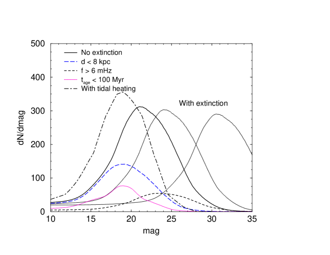
Figure 2.— The expected V-band magnitude distribution of the brightest member of the close white dwarf binaries resolved with LISA (solid line). This distribution must be corrected for Galactic extinction and we consider a simple prescription following Bahcall & Soneira (1980); in decreasing brightness, the dashed lines show the magnitude distribution when CWDBs are assumed to be distributed uniformly in a thick disk with scale height $\sim$ 1.5 kpc, and the case in which the distribution is highly flattened, with scale height $\sim$ 200 pc, such that more are towards the galactic plane. In the latter case, the extinction is significant and presents a challenge for optical studies. It is more likely that the true distribution is somewhere between the two cases we have considered. We also expect a small fraction of CWDBs to be distributed in the halo and not be affected by extinction significantly. With a dot-dashed line, we show the magnitude distribution (with no extinction) when we include an increase in white dwarf luminosity by tidal heating; we have considered the maximum brightening here under the assumption of equal-mass binaries and following the approach in Iben et al. (1998). The long-dashed line shows the distribution of magnitudes for white dwarfs at distances less than 8 kpc, while the dotted lines show the magnitude distribution of white dwarf binaries with GW frequencies greater than $\sim$ 6 mHz.

2. LISA Measurements and Optical Follow-up

First, we will review CWDB detection with LISA and then move on to discuss aspects related to their optical light curves. Briefly, one observes the two GW components given by the quadrupole approximation in the principal polarization coordinate (Peters 1964)

$$h_{+}(t) = A\cos\left[2\pi\left(f+\frac{1}{2}\dot{f}t\right)t+\phi(t)\right]\times\left[1+\cos^{2}i\right]$$

$$h_{\times}(t) = -2A\sin\left[2\pi\left(f+\frac{1}{2}\dot{f}t\right)t+\phi(t)\right]\times\cos i$$

where $\cos i$ is the inclination angle of the binary with respect to the observer and $\phi(t)$ is the phase resulting from the Doppler phase due to the revolution of LISA around the Sun and an integral constant ($\phi_{0}$).

CWDBs are expected to have circular orbits due to tidal interaction in earlier evolutionary stages. The amplitude of the wave is given by

$$A=\frac{5}{96\pi^{2}}\frac{\dot{f}}{f^{3}D}\,,$$ (2)

where $D$ is the distance to the source. Note that the GW frequency ($=2/P_{\rm orb}$ where $P_{\rm orb}$ is the orbital period) for a circular orbit is related to the total mass $M_{1}+M_{2}$ and the separation $a$ of the binary via

$$f\approx 3.5\times 10^{-3}\left(\frac{M_{\rm tot}}{0.9M_{\sun}}\right)^{1/2}\left(\frac{a}{10^{5}{\rm km}}\right)^{-3/2}\;{\rm Hz}\,,$$ (3)

while the time variation of this frequency is

$$\dot{f}=\frac{96\pi^{8/3}}{5}{\tilde{M}}^{5/3}f^{11/3}$$ (4)

$$\approx 1.2\times 10^{-16}\left(\frac{\tilde{M}}{0.4M_{\sun}}\right)^{5/3}\left(\frac{M_{\rm tot}}{0.9M_{\sun}}\right)^{11/6}\left(\frac{a}{10^{5}{\rm km}}\right)^{-11/2}{\rm Hz}\;{\rm s}^{-1}\,,$$

when the chirp mass is given by ${\tilde{M}}=M_{1}^{3/5}M_{2}^{3/5}/(M_{1}+M_{2})^{1/5}$ and the total mass $M_{\rm tot}=M_{1}+M_{2}$.

With GW data, one can estimate a total of 8 separate quantities, $A$, $f$, $\dot{f}$, $\phi_{0}$, location ($\vec{n}$, 2 parameters), and the direction of the angular momentum, $\vec{L}$ (2 parameters), though these estimates are not independent. The orbital inclination angle is given by $\cos^{-1}(\vec{n}\cdot\vec{L})$. In terms of physical quantities of interest, with $A$, $f$, $\dot{f}$, one extracts $D$ and ${\tilde{M}}$; in addition to these parameters one also constraints a combination of $M_{\rm tot}$ and $a$ using the frequency information following Eq. 3. Note that the relations (2) and (4) are given for Newtonian point particles as corrections for the finiteness of the stars are not significant.

The localization of binaries with LISA observations is discussed in Cutler (1998) for monochromatic sources (with $\dot{f}=0$), and in Takahashi & Seto (2002) for general observational situations. Following the Fisher matrix calculation in the latter paper, in Fig. 1, we show the distribution of error boxes for the binary locations extracted from the LISA data, for observations of 1, 3 and 5 years’ duration. To produce Fig. 1, we performed a Monte-Carlo analysis for 3000 Galactic CWDBs with $f>3$mHz, distributed in the Galaxy according to

$$\rho(R,z)=\rho_{0}{\rm sech}\left(\frac{|z|}{z_{0}}\right)^{2}\exp\left(-\frac{R}{R_{0}}\right)\,,$$ (5)

with $z_{0}=200$ pc and $R_{0}=2.5$ kpc (as in Nelemans et al. 2001). The LISA noise curve is taken from Finn & Thorne (2000) and the chirp mass distribution, as a function of GW frequency, is generated for the Galaxy using the same numerical codes used in Farmer & Phinney (2003), with a constant star formation rate over the past 10 Gyr, and other parameters as for their preferred Model A.

The locations for Fig. 1 were determined concurrently with the six other binary parameters. The parameter extraction can be considerably improved if a precise location for the binary is a priori known, especially if the observational duration is less than two years. This is certainly the case, for example, for the orientation of the orbit, which has strong a correlation with the location determination. A localization would traditionally come from optical observations and we consider this possibility here. While it may also be possible to localize CWDBs at other wavelengths of electromagnetic radiation, such as X-rays, we do not consider this possibility in the present discussion, but encourage others to do so.

Eclipses in the light curve as each white dwarf transits across the other will be a unique identifying signature of the binary. There will be two transits per orbital period. The WDs may or may not have similar surface temperatures, with the transits in which the second WD formed recently unlikely to have similar depths. Observationally WD–WD binaries are seen to be clustered around a mass ratio of unity (Maxted et al. 2002), so their radii are similar. Even if they are not, the worst-case scenario for central transit depth is of order a few tens of percent, for a large mass ratio and equal temperature (or large temperature ratio) system.

For a given binary, one can write down the probability for eclipse along our line of sight as

$${\rm Prob} = \frac{\int_{0}^{\cos i_{\rm min}}d(\cos i)}{\int_{0}^{1}d(\cos i)}=\cos i_{\rm min}\equiv\frac{R_{1}+R_{2}}{a}$$

$$\sim 0.30\left(\frac{f}{3.5{\rm mHz}}\right)^{2/3}\left(\frac{M_{\rm tot}}{0.5M_{\sun}}\right)^{-1/3}\left(\frac{R_{\rm WD}}{10^{4}{\rm km}}\right)\,,$$

(6)

where $R_{1}$ and $R_{2}$ are the WD radii and $a$ is the binary separation. The probability is substantial because $a$ is at most $\sim 5(R_{1}+R_{2})$ for spectrally resolved LISA binaries. This suggests that eclipses will be expected in the light curves of few tens of percent of all CWDBs resolved and localized with LISA at $f>3$mHz. We note however that this includes shallow grazing eclipses, and the probability for near-central transits is around half of the above value. The numerical estimate on the second line of Eq. 6 assumes equal mass, and thus equal size WDs of radii $R_{\rm WD}$.

Ignoring subtle effects such as the brightness distribution on the stellar surfaces, the optical light curves with eclipses, in general, allow one to establish the following parameters: $R_{1}/a\cos i$, $R_{2}/a\cos i$, and the ratio, $R_{1}/R_{2}$, if the transit durations can be measured. Unlike the GW data, which constrain the component masses through e.g. the chirp mass, transit light curves provide constraints on the objects’ physical sizes.

While there is a high probability of eclipse along our line of sight, we must consider what it will take to observe them. For this purpose, we first estimate the V-band apparent magnitude distribution of the brightest member of the CWDBs following the same mass and age distributions that were used for the calculation in Fig. 1. We summarize our results in Fig. 2. The luminosities are calculated based on age distributions, as a function of mass, by taking in to account WD cooling based on numerical fits to results of Blöcker (1995) and Driebe et al. (1998) in Nelemans et al. (2001a). We take a uniform bolometric correction of -0.2 consistent with DA white dwarfs at 8000K with $\log g=8$, consistent with the age distribution (Rohrmann 2001); for a range of temperatures, the corrections are at the level of -0.1 to -0.5 and we ignore this distribution for simplicity given the large uncertainties in the extinction as discussed below. The distribution is normalized to a total of 3000 CWDBs that are expected to be localized with LISA at $f>3$mHz (Seto 2002). This number, however, is uncertain and can be up to $\sim$ 6000 in different models (e.g., Nelemans et al. 2001b). The number depends also on the observational period. To convert luminosities to apparent magnitudes, we distribute these binaries in our galaxy as in equation 5.

The magnitude distribution has a peak at V-band magnitudes between 20 and 23. Note that we have neglected extinction here. To understand the extent to which extinction is important, we make use of the model in Bahcall & Soneira (1980). The spatial distribution of the CWDBs is important here. If the CWDB distribution trace the galactic disk as a thin disk, the extinction is significant: as shown with a dot-dashed line in Fig. 2, with $z_{0}=200$ pc in equation 5 the extinction can be high as 10 magnitudes, especially towards the galactic center where most CWDBs will be located. If the vertical distribution is allowed to expand, such as to a thick disk with $z_{0}=1.5$ kpc, then the extinction, on average, is about 3 magnitudes and the resulting modification still allows for a substantial number of binaries brighter than 25th magnitude. Such a thick disk has been suggested to explain the presence of high-velocity white dwarfs (e.g., Reid et al. 2001).

While extinction becomes a significant problem for the optical identification of CWDBs, there is an additional effect resulting from tidal heating in close binaries that can potentially increase their luminosities (Iben et al. 1998). For our standard case, with no extinction, we calculate the distribution of magnitudes with luminosities corrected for tidal brightening. For simplicity, we consider the maximum brightening given in Iben et al. (1998), again assuming equal mass binaries, as a function of the orbital period. With a gain of $\sim$ 3 magnitudes in the overall distribution, there is also a substantial increase in the number of binaries brighter than 20th magnitude. In general, tidal heating is not likely to be uniform and could produce hot-spots, which would in turn produce features in the light curve. Radiation from the companion star would produce similar effects.

In practice, the optical follow-up studies of LISA error boxes can be conducted as a two step process. First, the gravitational waves provide information related to the period and the phase, which is adequate to determine when eclipses in the optical light curve are expected. While the orbital periods are at the level of 500 seconds, for a quick identification, one can consider phased optical observations to identify the source with known period and eclipse phase. Once the source has been identified, more detailed light curves could be taken, to determine the orbital parameters, sampled at a few tens of seconds or less. Such a light curve would solidify the agreement between LISA’s period and phase with that of the optical data and help secure the identification exactly.

Since the magnitude distribution is expected to peak at magnitudes fainter than 25, detailed study may be limited to the tail of the distribution at the bright end. In general, with four-meter class telescopes, we expect that a detailed analysis of light curves would be possible for a magnitude limit of $\sim$ 22 to 23 with signal-to-noise ratios of order 10 in integration times of order 25 seconds. With phase matching, this signal-to-noise ratio can be improved. Given the follow-up error boxes number $\sim$ 3000, a dedicated telescope is not required for this purpose. Because the binary inclination and distance are determined in the GW parameter extraction process, and the brightest systems are also generally the closest (see Fig. 2), candidate bright-end CWDBs can be preferentially selected such that fewer boxes may need to be followed up. However, even non-detections would provide information on the presence of tidal heating for the highest-frequency binaries.

An imaging instrument capable of rapid (10–100 sec resolution) monitoring is needed. The field of view should be at the level of a square degree or more to match the error box sizes. Searches with smaller field of view instruments would be time-consuming. Visual magnitude limits of 25 or 26, in 25 second or so time intervals, are desirable, and a brighter limit would cut down the number of detectable sources substantially. It is unlikely that such an instrument currently exists, but given the potential of LISA for CWDB science, its planning is warranted and can be considered for upcoming telescopes such as the Large Synoptic Survey Telescope (LSST), which, by design, has the desirable field-of-view for a project such as this.

Additional information on the binary could be extracted with spectroscopic studies that involve radial velocity measurements. The radial velocities will be substantial, around a few times 100 km s^-1. Time-resolved spectroscopy of faint WDs, with notoriously few suitable spectral lines, could prove difficult for all but the most nearby systems. However, time-averaged spectra will be able to provide information on WD temperatures, which can be used in combination with distance and magnitude information, as well as eclipse data, to put better constraints on the WD parameters.

To summarize, the Laser Interferometer Space Antenna (LISA) is expected to individually detect between $\sim$ 3000 and 6000 Galactic close white dwarf binaries (CWDBs) through their gravitational radiation at frequencies above 3 mHz. Most of these binaries will be localized with LISA data to an accuracy that ranges from tens of arcminutes to a few degrees. Due to the small binary separation, the light curves of a few tenths of these resolved CWDBs are expected to show eclipses. This will give a unique signature for identification in follow-up optical studies of LISA error boxes, because the orbital period and phase will be known from LISA data. To optically identify a substantial fraction of CWDBs that are crudely localized with LISA , one will require a rapid monitoring campaign capable of imaging a square degree or more at intervals of tens of seconds, down to magnitude levels between 20 to 25. While such a study can be carried out with four or more meter-class telescopes down to magnitude levels of 25, no instrument currently exists to image a wide-field of view of a square degree or more continuously with sufficient time resolution and we highly encourage an investment in this aspect given the scientific potential related to LISA data.

Acknowledgments: We thank Gijs Nelemans and Sterl Phinney for useful discussions. This work is supported by the Sherman Fairchild foundation and DOE DE-FG 03-92-ER40701 (AC).

References

- (1) Bahcall, J. N. & Soneira, R. M. 1980, ApJS, 44, 73
- Blöcker (1995) Blöcker, T. 1995, A&A, 299, 755
- (3) Cornish, N. & Larson, S. L. 2002, gr-qc/0206017
- Driebe et al. (1998) Driebe, T., SDchönberner, D., Blöcker, T. & Herwig, F. 1998, A&A, 339, 123
- (5) Cutler, C. 1998, Phys. Rev. D., 49, 2658
- (6) Farmer, A. J. & Phinney, E. S. 2003, astro-ph/0304393
- Finn & Thorne (2000) Finn, L. S. & Thorne, K. S. 2000, Phys. Rev. D, 62, 124021
- Hils, Bender, & Webbink (1990) Hils, D., Bender, P. L., & Webbink, R. F. 1990, ApJ, 360, 75
- (9) Iben, I., Tutukov, A. V. & Fedorova, A. V. 1998, ApJ, 503, 344
- (10) Maxted, P. F. L., Marsh, T. R. & Moran, C. K. J. 2002, MNRAS, 332, 745
- (11) Napiwotzki, R., Koester, D., Nelemans, G. et al. 2002, A&A, 386, 957
- Nauenberg (1972) Nauenberg, M. 1972, ApJ, 175, 417
- (13) Nelemans, G., Yungelson, L. R. & Portegies Zwart, S. F. 2001, A&A, 375, 890
- (14) Nelemans, G., Yungelson, L. R., Portegies Zwart, S. F., Verbunt, F. 2001, A&A, 365, 491
- (15) Peters, P. C. 1964, Phys. Rev. B. 136, 1224
- Reid et al. (2001) Reid, I. N., Sahu, K. C. & Hawley, S. L. 2001, ApJ, 559, 942
- (17) Rohrmann, R. D. 2001, MNRAS, 323, 699
- (18) Seto, N. 2002, MNRAS, 333, 469
- (19) Takahashi, R. & Seto, N. 2002, ApJ, 575, 1030