Cosmological variation of deuteron binding energy, strong interaction and quark masses from big bang nucleosynthesis

Abstract

We use Big Bang Nucleosynthesis calculations and light element abundance data to constrain the relative variation of the deuteron binding energy since the universe was a few minutes old, $\delta Q=Q(BBN)-Q(present)$. Two approaches are used, first treating the baryon to photon ratio, $\eta$, as a free parameter, but with the additional freedom of varying $\delta Q$, and second using the WMAP value of $\eta$ and solving only for $\delta Q$. Including varying $Q$ yields a better fit to the observational data than imposing the present day value, rectifying the discrepancy between the ${}^{4}He$ abundance and the deuterium and ${}^{7}Li$ abundances, and yields good agreement with the independently determined $\eta_{WMAP}$. The minimal deviation consistent with the data is significant at about the 4-$\sigma$ level; $\delta Q/Q=-0.019\pm 0.005$. If the primordial ⁴He abundance lies towards the low end of values in the literature, this deviation is even larger and more statistically significant. Taking the light element abundance data at face-value, our result may be interpreted as variation of the dimensionless ratio $X=m_{s}/\Lambda_{QCD}$ of the strange quark mass and strong scale: $\delta X/X=(1.1\pm 0.3)\times 10^{-3}$. These results provide a strong motivation for a more thorough exploration of the potential systematic errors in the light element abundance data.

Pacs numbers: 26.35.+c, 21.10.Dr, 98.80.Ft

I Introduction

Recent astronomical data suggest a possible variation of the fine structure constant $\alpha=e^{2}/\hbar c$ at the $10^{-5}$ level over a time-scale of 10 billion years, see alpha (a discussion of other limits can be found in Ref. uzan and references therein). Naturally, these data motivated more general discussions of possible variations of other constants. Unlike for the electroweak forces for the strong interaction, there is generally no direct relation between the coupling constants and observable quantitites. In recent papers FS ; DF ; FS1 , we presented general discussions on the possible influence of the strong scale variation on primordial Big Bang Nucleosynthesis (BBN) yields, the Oklo natural nuclear reactor, quasar absorption spectra and atomic clocks. Here we continue this work, concentrating on BBN.

One can only measure variations of dimensionless parameters. Big Bang Nucleosynthes is sensitive to a number of fundamental dimensionless parameters including the fine structure constant $\alpha$ , $\Lambda_{QCD}/M_{Plank}$ and $m_{q}/\Lambda_{QCD}$ where $m_{q}$ is the quark mass and $\Lambda_{QCD}$ is the strong scale determined by a position of the pole in the perturbative QCD runnung coupling constant. In this work we search for any possible variation of $m_{q}/\Lambda_{QCD}$ because there is a mechanism which provides a very strong sensitivity of BBN to this parameter.

The first and most crucial step in BBN is the process $p+n\rightarrow d+\gamma$. The synthesis starts at $t\geq 3$ sec. when the temperature goes down below $T\leq 0.6$ MeV and lasts until $t\leq 6$ min. when the temperature becomes $T\leq 0.05$ MeV. The reaction rate for the above process defines all subsequent processes and final primordial abundances of light elements. Amongst the factors that can influence the reaction rate, the most significant seems to be a variation of the deuteron binding energy (this variation was discussed in Refs. Dys71 ; Davies ; Barrow ; PP91 ; FS ; FS1 ; Kneller ; Yoo ). Indeed, the equilibrium concentration of deuterons and the inverse reaction rate depend exponentially on it. Moreover, the deuteron is a shallow bound level. Therefore the relative variation of the deuteron binding $Q$ is much larger than the relative variation of the strong potential $U$, i.e. $\delta Q/Q>>\delta U/U$. As a result the variations in the strong interaction may be most pronounced via the deuteron binding energy. We also take into account the effect of variation of the virtual level in the neutron-proton system, which is even more sensitive to the variation of the strong interaction.

The question we address here is whether or not existing observations of the primordial abundances of the light elements suggest any change in the deuteron binding energy at the time of BBN.

To do so, we use a compliation of light element abundance data from the literature for ⁴He, ⁷Li and D/H. As we show later, the currently greater experimental precision on ⁴He results in that element dominating our results. The other 2 light elements nevertheless provide important consistency checks.

The data we use for ⁴He is presented in Table 1 and comprised 14 surveys giving estimates for the primordial value, Y_p, derived using, or by extrapolation to, low metallicity in each case. There is clear evidence for significant scatter amongst these 14 values, presumably due to unquantified systematics, or if not, intrinsic inhomogeneities. The dominance by ⁴He, or indeed by any single element, unfortunately increases susceptibility to systematic errors, and we have therefore attempted to explore the effect of these in several ways.

Firstly, in order to make best use of all the available ⁴He data, we add a constant term to each of the statistical errors on Y_p, such that that the normalised $\chi^{2}$ for all 14 points about the weighted mean value is equal to unity. This approach is equivalent to the assumption that all 14 estimates of Y_p are unbiased and Gaussian distributed, but that there is an additional systematic component to the statistical error which is different (and hence random) for each estimate.

Second, as shown later, smaller values of Y_p are less consistent with $\delta Q/Q=0$ than larger values. Thus we carry out a re-analysis using a subset of the Y_p’s, taking only the highest values such that the normalised $\chi^{2}$ about the weighted mean value is equal to unity, without increasing the individual errors by a constant, as described above. This procedure selects 9 values from the original 14. In doing this, we are exploring the consequence of there being strong systematics for the small Y_p’s, and little or none for the high values. This is conservative, in the sense that we are minimising our estimate for $\delta Q/Q$.

Finally, in order to obtain some estimate of the plausible range on our estimate of $\delta Q/Q$, we perform the converse analysis, subsetting the data by discarding high values of Y_p, again such that the normalised $\chi^{2}$ about the weighted mean value is equal to unity. This leaves 9 points. The two samples thus overlap.

Table 1: Data on the primordial ⁴He mass fraction

$Y_{p}$	Ref.
0.2391 $\pm$ 0.0020	lppc
0.2384 $\pm$ 0.0025	ppl
0.2371 $\pm$ 0.0015	pp
0.2443 $\pm$ 0.0015	ti
0.2351 $\pm$ 0.0022	ppl1
0.2345 $\pm$ 0.0026	ppr
0.244 $\pm$ 0.002	ti1
0.243 $\pm$ 0.003	itl
0.232 $\pm$ 0.003	os
0.240 $\pm$ 0.005	itl1
0.234 $\pm$ 0.002	oss
0.244 $\pm$ 0.002	it
0.242 $\pm$ 0.009	it1
0.2421$\pm$ 0.0021	izth03

The data on deuterium abundances D/H from quasar absorption systems were selected according two criteria:
(i) Metallicity must be low, so as to more closely reflect primordial value: [Si/H] or [O/H] less than or equal to -2.0.
(ii) Must be detection, not upper limit.
These requirements leave only five data points listed in Table 2

Table 2: Data on the primordial deuterium abundance

QSO	z(abs)	D/H$\times 10^{-5}$	[Si/H]	Ref.
Q1009+299	2.504	4.0 $\pm$ 0.65	-2.53	bt
PKS1937-1009	3.572	3.25$\pm$ 0.3	-2.26 [O/H]	bt1
HS0105+1619	2.536	2.5 $\pm$ 0.25	-2.0	omear
Q2206-0199	2.076	1.65 $\pm$ 0.35	-2.23	petb
Q1243+3047	2.526	2.42 +0.35 - 0.25	-2.77 [O/H]	kirk

The data for Lithium primordial abundance are shown in Table 3. Here $A=Log(Y_{Li})+12.$

Table 3: Data on the primordial Li/H abundance

$A$	Ref.
2.09 +0.11-0.12	rbofn
2.35 $\pm$ 0.1	boni
2.36 $\pm$ 0.12	bdsk
2.34 $\pm$ 0.056$\pm$0.06	bonal
2.07 + 0.16 - 0.04	syb
2.22 $\pm$ 0.20	thor
2.4 $\pm$ 0.2	pswn
2.5 $\pm$ 0.1	tv

Applying the first procedure described above, in order to obtain $\chi^{2}/N=1$, we have to add to the individual $\sigma$’s 0.0017 for helium points, $0.344\times 10^{-5}$ for deuterium points, and 0.028 for lithium points. For the weighted mean values we obtain

$$Y_{p}=0.2393\pm 0.0011,$$ (1)

$$Y_{D}=(2.63\pm 0.31)\times 10^{-5},$$ (2)

and

$$A=2.315\pm 0.051.$$ (3)

The latter value corresponds to the following lithium abundance

$$Y_{Li}=(2.02\pm 0.22)\times 10^{-10}.$$ (4)

The second and the third procedures are meaningful only for the helium points. The number of deuterium points is too small and the lithium data points are the least scattered. We need only 20% increase in individual uncertainties to bring $\chi^{2}/N$ to 1 for the lithium data. In addition, the deuterium and the lithium data do not produce a significant contribution in determination of $\delta Q/Q$ which is entirely dominated by the helium data due to their high accuracy.

Keeping 9 upper points for the helium mass fraction data, that give $\chi^{2}/N=0.94$, we obtain for the weighted mean value

$$Y_{p}=0.2424\pm 0.0008.$$ (5)

If we keep 9 lower points, we obtain

$$Y_{p}=0.2363\pm 0.0008,$$ (6)

which is significantly lower than both in Eq.(5) and Eq. (1).

II The BBN equations

We use the standard BBN set of equations that describe the time development of the abundances of the elements in an expanding Universe wago

$$\frac{\dot{R}}{R}=H=\sqrt{\frac{8\pi}{3M_{P}^{2}}\rho_{T}},$$ (7)

$$\frac{\dot{n_{B}}}{n_{B}}=-3H,$$ (8)

$$\dot{\rho_{T}}=-3H(\rho_{T}+p_{T}),$$ (9)

$$\dot{Y}_{i}=\sum_{j,k,l}N_{i}\left(\Gamma_{kl\rightarrow ij}\frac{Y_{l}^{N_{l}}Y_{k}^{N_{k}}}{N_{l}!N_{k}!}-\Gamma_{ij\rightarrow kl}\frac{Y_{i}^{N_{i}}Y_{j}^{N_{j}}}{N_{i}!N_{j}!}\right),$$ (10)

$$n_{-}-n_{+}=\frac{n_{B}}{T^{3}}\sum_{j}Z_{j}Y_{j},$$ (11)

where $n_{B}$ is the density of baryons, $Y_{i}$ is the abundance of the element ${}^{A_{i}}Z_{i}$. The right-hand side of Eq.(10) corresponds to a reaction

$$N_{i}(^{A_{i}}Z_{i})+N_{j}(^{A_{j}}Z_{j})\leftrightarrow N_{k}(^{A_{k}}Z_{k})+N_{l}(^{A_{l}}Z_{l}).$$ (12)

$\rho_{T}$ and $p_{T}$ denote total energy density and pressure, respectively,

$$\rho_{T}=\rho_{\gamma}+\rho_{e}+\rho_{\nu}+\rho_{B},$$ (13)

$$p_{T}=p_{\gamma}+p_{e}+p_{\nu}+p_{B}.$$ (14)

Eq.(7) defines the expansion rate. Eq.(8) defines the change in time of the baryon density, and the rate equation Eq.(10) defines the time evolution of the abundances and their final values after freeze-out. The last Eq.(11), where $n_{-}$ and $n_{+}$ are the densities of electrons and positrons, is the condition of electro-neutrality that defines a chemical potential of electrons.

III Effect of the deuteron binding energy variation

The sensitivity of the reaction rate $\Gamma_{\gamma d\leftrightarrow pn}$ to parameters of the strong interaction in general, and to the deuteron binding energy in particular, comes from two sources. First, the reaction rate $\Gamma_{\gamma d\leftrightarrow pn}$ depends exponentially on the deuteron binding energy $Q$. Second, the cross section of the reaction $np\rightarrow\Gamma_{\gamma d}$ is very sensitive to the position of the virtual level with the energy $\epsilon_{v}=0.07MeV$. Any change in the strong NN-potential causing a shift in the deuteron binding energy $Q$ will change the position of the virtual level $\epsilon_{v}$ as well. The relation between $\delta Q$ and $\delta\epsilon_{v}$ can be obtained using the fact that both a real level and a virtual one are close to $E=0$. The relation is (see Appendix)

$$\frac{\delta\epsilon_{v}}{\sqrt{\epsilon_{v}}}=-\frac{\delta Q}{\sqrt{Q}}.$$ (15)

The cross section for $n+p\rightarrow d+\gamma$ reaction can be found in textbooks seg . In the leading order in $Q/\epsilon_{v}$ the product of the cross section and the velocity is proportional to

$$\sigma v\sim Q^{5/2}/\epsilon_{v}.$$

Thus, in linear order in $\delta Q$ we have the following modification of the reaction rate

$$\Gamma_{np\rightarrow d\gamma}\rightarrow\Gamma_{np\rightarrow d\gamma}\left(1+\left(5/2+\sqrt{\frac{Q}{\epsilon_{v}}}\right)\frac{\delta Q}{Q}\right).$$ (16)

We should note, however, that according to our BBN calculations the direct effect of the deuteron binding energy variation (due to the exponential dependence of the inverse reaction rate $d\gamma\rightarrow np$) is more important than the variation of the cross-section $np\rightarrow d\gamma$ Eq.(16) .

We modified one of the standard BBN codes kawano in such a way that $Q$ can be changed for this reaction. Varying $Q$ changes the abundances of all three elements under discussion. In Fig.1 we plot the abundance of D, the mass fraction of ⁴He, and the abundance of ⁷Li, as functions of $Q$ at the value of the baryon to photon ratio $\eta=6.14\times 10^{-10}$ found from anisotropy of cosmic microwave background benn

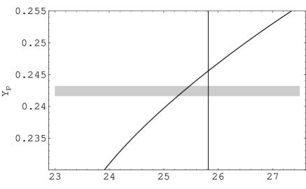
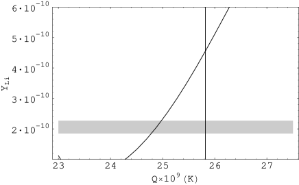
Figure 1: The light elements abundances as a functions of the deuteron binding energy $Q$ for $\eta_{WMAP}=6.14\times 10^{-10}$. The vertical line shows the present value of $Q=25.82\times 10^{9}$ K. The shaded regions illustrate the 1$\sigma$ range in the data. For helium the high $Y_{p}$ value (Eq.5) is shown.

From Fig 1. we see that the deuterium abundance is not very sensitive to $Q$. The data are fully compatible with the present value of the deuteron binding energy. Such a poor sensitivity can be explained by relatively large error bars for the deuterium abundance.

The data on ⁴He, in contrast, show strong sensitivity to the deuteron binding energy favoring for lower $Q$ during primordial nucleosynthesis. The data on ⁷Li also favoring for lower $Q$ approximately for the same $\delta Q$ as ⁴He.

The above Figure 1 give a qualitative picture of the dependence of light element abundances on the deuteron binding energy. In order to obtain more quantitative results we analyse the likelihood functions as functions of $Q$ and $\eta$.

III.1 The likelihood functions

The likelihood function for the abundances have been choosen in the form

$$Lf(\eta,Q)=\exp(-\frac{1}{2}\sum_{ij}(Y^{th}_{i}(\eta,Q)-Y^{ex}_{i})w_{ij}$$

$$\times(Y^{th}_{j}(\eta,Q)-Y^{ex}_{j})).$$ (17)

Here the sum goes over three light elements, $w_{ij}$ is the inverse error matrix that was calculated using the approach proposed in Ref. flsv . The errors in theoretical values of the abundances can be found from the uncertainties in the reaction rates

$$\delta Y_{i}^{th}=Y^{th}_{i}\sum_{k}\lambda_{ik}\frac{\Delta R_{k}}{R_{k}},$$ (18)

where $\Delta R_{k}$ are the reaction rate errors, and

$$\lambda_{ik}=\frac{\partial\,{\rm ln}Y^{th}_{i}}{\partial\,{\rm ln}R_{k}}$$

are the logarithmic derivatives. The error matrix $\sigma_{ij}$ can be calculated then by

$$\sigma_{ij}^{2}=Y^{th}_{i}Y^{th}_{j}\sum_{k}\lambda_{ik}\lambda_{jk}\left(\frac{\Delta R_{k}}{R_{k}}\right)^{2}.$$ (19)

The uncertainties in the experimental data (1), (2), (4) should be added to the diagonal matrix elements of the error matrix (19)

$$\sigma^{tot\,2}_{i}=\sigma^{2}_{ii}+\sigma^{ex\,2}_{i}.$$ (20)

For ⁴He $\sigma^{tot}$ differs from $\sigma^{ex}$ insignificantly, while for D and especially for ⁷Li $\sigma_{ii}$ and $\sigma^{ex}_{i}$ are comparable. If we neglect the correlations then the matrix $w_{ij}$ is diagonal and equal to

$$w_{ii}=1/\sigma^{tot\,2}_{i}.$$

In this case we can present the likelihood function (III.1) as a product of three individual functions $Lf(\eta,Q)=Lf_{D}(\eta,Q)Lf_{He}(\eta,Q)Lf_{Li}(\eta,Q)$. The equations

$$Y_{i}(\eta,Q)=Y^{ex}_{i}$$ (21)

defines three lines in $\eta-Q$ plane where the individual likelihood functions are equal to one. And the equations

$$(Y_{i}(\eta,Q)-Y^{ex}_{i})^{2}=\sigma^{tot\,2}_{i}$$ (22)

define 1$\sigma$ ranges around these lines for each element. These ranges are shown in Fig 2.

Figure 2: 1$\sigma$-ranges around the maxima of individual likelihood functions. The solid lines show 1$\sigma$-ranges for D, the dashed lines are for ⁴He (using $Y_{p}$ from Eq.5), and the dot-dashed lines are for ⁷Li. For lithium, there are 2 solutions for $\eta$ and $Q$, hence the shape of the error contours is more complicated.

The slope of the deuterium range is smaller than that of helium and lithium reflecting smaller sensitivity in $Q$ and higher sensitivity in $\eta$. .

In contrast, the helium range goes almost vertically reflecting high sensitivity of the helium fraction to $Q$ and low sensitivity to $\eta$. This low sensitivity to $\eta$ can be explained by a large helium binding energy. Only gamma’s with the energy $E_{\gamma}>$20 MeV can significantly change the number of helium nuclei. At any $\eta$ the number of such $\gamma$-quanta is small at the BBN temperature. We can, therefore, expect the low sensitivity of the helium mass fraction to $\eta$.

The Lithium range has two distinct branches corresponding to two different solutions of Eq.(21) for $\eta$ at given $Q$. All three ranges intersect near $\eta=6.5$ and $Q=25$. One can expect that the general likelihood function (III.1) will have a maximum in this region. Indeed, we found the maximum of $Lf(\eta,Q)$ at the point $\eta_{m}=(6.51\,+\,0.77\,-\,0.66)\times 10^{-10}$ and $Q_{m}=(25.26\pm 0.20)\times 10^{9}$K. Fig. 3 shows 1$\sigma$ elliptic boundary near the maximum. The long axis of the ellipsis is almost vertical. Therefore,

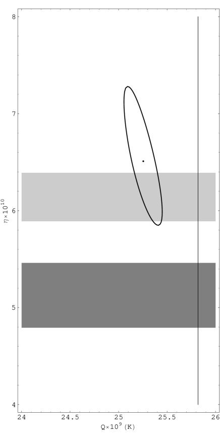
Figure 3: 1$\sigma$-range about the maximum of $Lf(\eta,Q)$ (again using Y_p from Eq.5). The lighter shaded region shows CMB-WMAP data for $\eta$. The darker shaded region is the 1$\sigma$-range for $\eta$ from BBN calculations using the present-day value of the deuteron binding energy, $Q=25.82$. A lower value of Y_p will produce a larger deviation between the $\eta_{WMAP}$ and $\eta_{BBN}$.

the correlation between $\Delta\eta$ and $\Delta Q$ is not significant. Comparing Fig. 3 and Fig. 2 one can conclude that the error $\Delta Q$ is determined mostly by ⁴He mass fraction data. It is interesting to note that $\eta_{m}$ is compatible with the one found from recent CMB anisotropy measurementbenn . The dark shadow region shows the 1$\sigma$ range for $\eta$ fitted from BBN only at present value of $Q=25.82$ K.

III.2 Constraint from CMB anisotropy measurements

The value of $\eta$ found from CMB anisotropy measurements

$$\eta_{0}=(6.14\pm 0.25)\times 10^{-10}$$

has rather high accuracy. It is natural to use the constraint from this measurement in our study of the deuteron binding energy effects. To do this we construct another likelihood function which is a function of $Q$ only.

$$L(Q)=\int_{-\infty}^{\infty}\exp(-\frac{(\eta-\eta_{0})^{2}}{2\sigma^{2}_{\eta}})Lf(\eta,Q)\,d\eta.$$ (23)

If we neglect nondiagonal elements in $w_{ij}$ we can construct the individual likelihood functions for D, ⁴He, and ⁷Li. They are constructed in the same way as (23) using instead of general function $Lf(\eta,Q)$ the individual ones $Lf_{D}(\eta,Q)$, $Lf_{He}(\eta,Q)$ , $Lf_{Li}(\eta,Q)$. These functions are plotted in Fig. 4 together with the general likelihood function (23)

Figure 4: Individual likelihood functions (23) for the light elements. From top to bottom: D, ⁴He (Eq.5), Li, and the combined datset.

From the deuterium likelihood function we found the position of the maximum and 1$\sigma$ deviations:

$$Q_{D}=(25.74+0.92-0.68)\times 10^{9}.$$ (24)

The shape near the maximum is apparently non-symmetric. The position of the maximum is fully compatible with the present value of $Q=25.82\times 10^{9}$ K. The helium likelihood function is much narrower (see the second panel from the top). It gives for the maximum and for the 1$\sigma$ the values

$$Q_{He}=(25.37\pm 0.13)\times 10^{9}.$$ (25)

This value lies below the present value of the binding energy. Finally, the lithium likelihood function has the maximum at

$$Q_{Li}=(24.88+0.43-0.59)\times 10^{9}.$$ (26)

The position of this maximum is compatible with the helium result.

The general likelihood function (23) is plotted in the lower panel in Fig. 4 The position of its maximum differs only slightly from the position given by the helium likelihood function.

$$Q_{BBN}=(25.34\pm 0.12)\times 10^{9}$$ (27)

It is interesting to compare the light element abundances for two values of the deuterium binding energies. In Fig. 5 we plotted the traditional curves for the light element abundances as a functions of $\eta$ for two values of $Q$. The dotted lines in the figures correspond to a present value of $Q_{present}=25.82\times 10^{9}$ K, while the solid curves correspond to a new value $Q_{BBN}=25.34\times 10^{9}$ K. Clearly, the new value $Q_{BBN}$ moves the curves closer to the data.

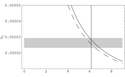
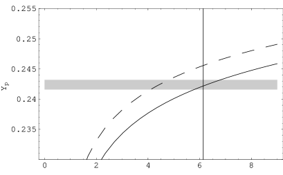
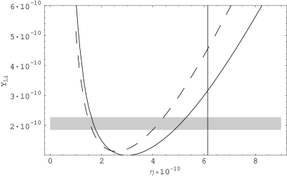
Figure 5: The predicted light element abundance yields as a function of $\eta$, for two values of the deuteron binding energy, $Q$. The dotted curve corresponds to the present value of $Q_{present}=25.82\times 10^{9}$ K. The solid curve corresponds to the new value of $Q=Q_{BBN}=25.34\times 10^{9}$ K. The vertical line corresponds to $\eta=6.14$ (WMAP value). The shaded regions is the 1$\sigma$-ranges for the observed light element abundances, where Y_p is from eq.5.

The result which we obtained may be presented as

$$\delta Q/Q=-0.019\pm 0.005,$$ (28)

where $\delta Q=Q_{BBN}-Q_{present}$. If we do not fix $\eta$ and try to fit it simulaneously with $Q$ we obtain

$$\delta Q/Q=-0.022\pm 0.008,\;\eta=(6.51+0.77-0.66)\times 10^{-10}.$$ (29)

The obtained $\eta$ is fully compatible with the one measured by WMAP.

These values of $\delta Q/Q$ and $\eta$ were obtained for high value of the helium mass fraction $Y_{p}$. If we use as an input the low value of $Y_{p}$ from (6) we obtain

$$\delta Q/Q=-0.048\pm 0.004,$$ (30)

If we fit both $\delta Q/Q$ and $\eta$ we obtain

$$\delta Q/Q=-0.059\pm 0.007,\;\eta=(7.55+0.91-0.75)\times 10^{-10}.$$ (31)

Finally if we use the value of $Y_{p}$ for ⁴He obtained using the whole sample of 14 points, with increased error bars, from Eq.(1), we obtain

$$\delta Q/Q=-0.033\pm 0.006,$$ (32)

and for $\delta Q/Q$ and $\eta$

$$\delta Q/Q=-0.042\pm 0.009,\;\eta=(7.00+0.85-0.72)\times 10^{-10}.$$ (33)

The results given in eqs.(28) and (30) therefore represent an estimate of the plausible range in $\delta Q/Q$. Despite the clear systematic uncertainties in the ⁴He data, and accepting the WMAP value of $\eta$ as being correct, $\delta Q/Q$ appears to deviate from zero by 4$\sigma$ (eq. 28) or greater (eqs. 30, 32).

The deuteron binding energy depends on the strong scale and quark masses. It is convenient to assume that $\Lambda_{QCD}$ is constant , and the quark mass is variable. This only means that we measure all energies in units of $\Lambda_{QCD}$ (and cross-sections in units $\Lambda_{QCD}^{-2}$). In Ref. FS1 we concluded that the deuteron binding energy is very sensitive to variation of the strange quark mass $m_{s}$ strange :

$$\frac{\delta(Q/\Lambda_{QCD})}{(Q/\Lambda_{QCD})}=-17\frac{\delta(m_{s}/\Lambda_{QCD})}{(m_{s}/\Lambda_{QCD})}$$ (34)

Combining eqs. (32) and (34) we obtain

$$\frac{\delta(m_{s}/\Lambda_{QCD})}{(m_{s}/\Lambda_{QCD})}=(1.1\pm 0.3)\times 10^{-3}$$ (35)

This equation may contain an additional factor (close to one) reflecting unknown theoretical uncertainty in eq. (34). Note that we obtain here variation at the level $10^{-3}$ while the limits on variation of $\alpha$ Bergstrom ; uzan and $\Lambda_{QCD}/M_{Plank}$ FS ; uzan are an order of magnitude weaker. This may serve as a justification of our approach.

IV Conclusion

Allowing the deuteron binding energy, $Q$, to vary in BBN appears to provide a better fit to the observational light element abundance data. Varying $Q$ simultaneously does two things; it resolves the internal inconsistency between ⁴He and the other light elements, and it also results in excellent independent agreement with the baryon to photon ratio determined from WMAP. (Fig. 5). However, the magnitude of the variation is sensitive primarily to the observed ⁴He abundance, which has the smallest relative statistical error. A systematic error in the abundance of ⁴He could imitate the effect of the deuteron binding energy variation, although one needs a systematic error which is very much greater than has been claimed in the most recent observational work.

We note that Izotov and Thuan izth03 , the most recent estimate for Y_p in our sample, argue that systematics are at most 0.6% for that survey. On the other hand, the possibility has also been explored that the creation of ⁴He in population III stars might mean that the true primordial ⁴He abundance is lower even than that seen in the most metal-poor objects salv . If so, the significance of the deviation of $\delta Q/Q$ from zero we report in this paper would be even larger.

These results hopefully provide an extremely strong motivation to obtain substantially better measurements of all the light elements, and to explore even more intensively, the possible sources of systematic errors.

Appendix

Let $U_{0}(r)$ be a critical depth potential for which the binding energy $Q=0$, and $U_{t}(r)$ a potential for a proton neutron system in a triplet state producing a deuteron with small binding energy $Q=2.22$ MeV. If we add to the deuteron Hamiltonian a perturbation

$$\delta U_{\lambda}(r)=\lambda(U_{0}(r)-U_{t}(r)),$$

then, variation of $\lambda$ from 0 to 1 will move the binding energy $Q$ from 2.22 MeV to 0. From a virial theorem for a quantum system we have

$$\frac{dE}{d\lambda}=\int_{0}^{\infty}(U_{0}(r)-U_{t}(r))\chi^{2}(r)dr,$$ (36)

where $\chi(r)$ is the radial s-wave function. For simplicity we neglect the d-wave contribution. For $Q\rightarrow 0$ the main contribution into normalization integral for $\chi(r)$ comes from the region outside of the nuclear forces radius $R$. The normalization integral can be presented as sum of contributions from inner and outer regions

$$\int_{0}^{R}\chi^{2}(r)dr+b^{2}\int_{R}^{\infty}e^{-2\gamma r}dr=1,$$ (37)

where $\gamma=\sqrt{\frac{m_{p}|E|}{\hbar^{2}}}$. At $|E|\rightarrow 0$ the second integral dominates giving $b^{2}=2\gamma$. Separating the $E$-dependence of the normalization factor in $\chi(r)$ we can rewrite Eq.(36) as

$$\frac{dE}{\sqrt{|E|}}=d\lambda\,2\sqrt{\frac{m_{p}}{\hbar^{2}}}\int_{0}^{\infty}(U_{0}(r)-U_{t}(r))\tilde{\chi}^{2}(r)dr,$$ (38)

where $\tilde{\chi}(r)$ is practically independent on $E$ inside the potential well (where $E<<U$) and $\tilde{\chi}(r)=e^{-2\gamma r}\rightarrow 1$ at $r>R$ when $|E|\rightarrow 0$ . Integrating the left hand side of Eq.(38) over $E$ from $-Q$ to 0 and the right hand side of Eq.(38) over $\lambda$ from 0 to 1 we obtain

$$Q=\frac{m_{p}}{\hbar^{2}}\left(\int_{0}^{\infty}(U_{0}(r)-U_{t}(r))\tilde{\chi}^{2}(r)dr\right)^{2}.$$ (39)

The Eq.(39) shows that the position of a shallow bound level depends quadratically on the difference between the actual depth of the potential and the critical one. For a square well $Q=\frac{\pi^{2}(U-U_{0})^{2}}{16U_{0}}$, $U_{0}=\frac{\pi^{2}\hbar^{2}}{4m_{p}R^{2}}$.

In fact, the Eq.(39) is valid not only for the energy of a bound level but for the energy of a virtual level as well. The integration in Eq.(39) is over the region $r<R$ where the function $\tilde{\chi}^{2}(r)$ is insensitive to the energy $E$, and the quadratic dependence on $U-U_{0}$ guarantees the validity of Eq.(39) for both $U<U_{0}$ and $U>U_{0}$. Thus, for the energy of the virtual level we have

$$\epsilon_{v}=\frac{m_{p}}{\hbar^{2}}\left(\int_{0}^{\infty}(U_{0}(r)-U_{s}(r))\tilde{\chi}^{2}(r)dr\right)^{2},$$ (40)

where $U_{s}(r)$ is the potential for a singlet states. We have both $Q<<U$ and $\epsilon_{v}<<U$. This means that the difference between the triplet and singlet potentials is not large. Assuming that the changes in the triplet and singlet potentials are the same we obtain for the changes in $Q$ and $\epsilon_{v}$ the relation

$$\frac{\delta\epsilon_{v}}{\sqrt{\epsilon_{v}}}=-\frac{\delta Q}{\sqrt{Q}}.$$ (41)

This equation also holds for the effect produced by variation of the proton mass ( the dominating effect comes from variation of $U_{0}$).

References

- (1) J. K. Webb , V.V. Flambaum, C.W. Churchill, M.J. Drinkwater, and J.D. Barrow,M.J. Drinkwater, and J.D. Barrow, Phys. Rev. Lett., 82, 884-887, 1999. J.K. Webb, M.T. Murphy, V.V. Flambaum, V.A. Dzuba, J.D. Barrow,C.W. Churchill, J.X. Prochaska, and A.M. Wolfe, Phys. Rev. Lett. 87, 091301 -1-4 (2001). M. T. Murphy, J. K. Webb, V. V. Flambaum, V. A. Dzuba, C. W. Churchill, J. X. Prochaska, J. D. Barrow and A. M. Wolfe, Mon.Not. R. Astron. Soc. 327, 1208 (2001) ; astro-ph/0012419. M.T. Murphy, J.K. Webb, V.V. Flambaum, C.W. Churchill, and J.X. Prochaska. Mon.Not. R. Astron. Soc. 327, 1223 (2001); astro-ph/0012420. M.T. Murphy, J.K. Webb, V.V. Flambaum, C.W. Churchill, J.X. Prochaska, and A.M. Wolfe. Mon.Not. R. Astron. Soc. 327,1237 (2001); astro-ph/0012421. M. T. Murphy, J. K. Webb, V. V. Flambaum, Mon.Not. R. Astron. Soc. 345, 609 (2003).
- (2) J. Uzan, Rev. Mod. Phys. 75, 403 (2003).
- (3) V.V. Flambaum, E.V. Shuryak, Phys. Rev. D65, 103503 (2002).
- (4) V.F. Dmitriev, V.V. Flambaum, , Phys. Rev. D67, 063513 (2003).
- (5) V.V. Flambaum, E.V. Shuryak, Phys. Rev. D67, 083507 (2003).
- (6) F.J. Dyson, Sci. Am. 225, 51 (1971).
- (7) J.D. Barrow, Phys. Rev. D35, 1805 (1987).
- (8) T. Pochet, J.M. Pearson, J. Beaudet, H. Reeves, Astron. Astrophys. 243, 1 (1991).
- (9) , J.J Yoo, R.J. Scherrer , Phys.Rev. D67 (2003) 043517, astro-ph/0211545.
- (10) J.P. Kneller, G.C. McLaughlin, nucl-th/0305017.
- (11) P. Davies, J. Phys.A: Gen.Phys. 5, 1296 (1972).
- (12) V. Luridiana, A. Peimbert, M. Peimbert, M. Cervino astro-ph/0304152.
- (13) A. Peimbert, M. Peimbert, V. Luridiana, Astrophys. J 565 (2002) 668.
- (14) A. Peimbert, M. Peimbert, Revista Mexicana de Astronoma y Astrofisica (Serie de Conferencias), 12 (2002) 250.
- (15) T. X. Thuan, Y.I. Izotov Space Science Reviews 100 (2002) 263.
- (16) A. Peimbert, M. Peimbert, V. Luridiana Revista Mexicana de Astronoma y Astrofisica (Serie de Conferencias), 10 (2001) 148.
- (17) A. Peimbert, M. Peimbert, M.T. Ruiz Astrophys. J, 541 (2000) 688.
- (18) T. X. Thuan, Y.I. Izotov Space Science Reviews, 84 (1998) 83.
- (19) Y.I. Izotov, T. X. Thuan, V.A. Lipovetsky Astrophys. J. Suppl., 108 (1997) 1.
- (20) K.A. Olive, G. Steigman Astrophys. J. Suppl., 97 (1995) 49.
- (21) Y.I. Izotov, T. X. Thuan, V.A. Lipovetsky Astrophys. J., 435 (1994) 647.
- (22) K.A. Olive, G. Steigman, E.D. Skillman Astrophys. J., 483 (1997) 788.
- (23) Y.I. Izotov, T. X. Thuan Astrophys. J., 500 (1998) 188.
- (24) Y.I. Izotov, T. X. Thuan Astrophys. J., 497 (1998) 227.
- (25) Yuri I. Izotov and Trinh X. Thuan, astro-ph/0310421.
- (26) S. Burles and D. Tytler, Astrophys. J. 507 (1998) 732.
- (27) S. Burles and D. Tytler, Astrophys. J. 499 (1998) 689.
- (28) J.M. O’Meara, et al., Astrophys. J. 552 (2001) 718.
- (29) M. Pettini and D. Bowen, Astrophys. J. 560 (2001) 41.
- (30) D. Kirkman, et al., astro-ph/ 0302006.
- (31) S.G. Ryan, T.C. Beers, K.A. Olive, B.D. Fields, J.E. Norris, Astrophys. J. 530 (2000) L57.
- (32) P. Bonifacio and P. Molaro, Mon. Not. Roy. Astron. Soc. 285 (1997) 847, S. Vauclair, C. Charbonnel, Astronomy and Astrophysics 375 (2001) 70.
- (33) P. Bonifacio, Astronomy and Astrophysics 395 (2002) 515, A.M. Boesgaard, C.P. Deliyannis, A. Stephens, J.R. King, Astrophys. J. 193 (1998) 206.
- (34) P. Bonifacio et al., Astronomy and Astrophysics 390 (2002) 91.
- (35) T.K. Suzuki, Y. Yoshi, T.C. Beers, Astrophys. J. 540 (2000) 103.
- (36) J.A. Thorburn, Astrophys. J. 421 (1994) 318.
- (37) M.H. Pinsonneault, G. Steigman, T.P. Walker, V.K. Narayanan, astro-ph/0105439.
- (38) S. Theado, S. Vauclair, Astronomy and Astrophysics 375 (2001) 70.
- (39) R.V. Wagoner, W.A. Fowler, and F. Hoyle, Astrophys. J. 148 (1967) 3; R.V. Wagoner, Astrophys. J. Suppl. 18 (1969) 247; R.V. Wagoner, Astrophys. J. 179 (1973) 343.
- (40) Emilio Segre, Nuclei and Particles, Second Edition, W.A. Benjamin, Inc., 1977.
- (41) L. Kawano, preprint FERMILAB-Pub-88/34-A; preprint FERMILAB-Pub-92/04-A.
- (42) C.L. Bennett et al., astro-ph/0302207; D.N. Spergel et al., astro-ph/0302209.
- (43) G. Fiorentini, E. Lisi, S. Sarkar and F.L. Villante, Phys. Rev. D58 (1998) 063506.; E. Lisi, S. Sarkar and F.L. Villante, Phys. Rev. D59 (1999) 123520.
- (44) S.R. Beane and M.J. Savage, hep-ph/0206113.
- (45) L.D. Landau, E.M. Lifshits. Quantum Mechanics, Theoretical Physics, Volume 3 (Nauka, Moscow,1974).
- (46) J.Gasser and H.Leutwyler, Phys.Rep.87 (1982) 77. S. J. Dong, J. F. Lagae and K. F. Liu, Phys. Rev. D 54, 5496 (1996), (hep-ph/9602259).
- (47) The enhanced sensitivity of the deuteron binding energy to the strong qurak mass is explained by four factors FS1 : 1) deuteron is the shallow level which may be eliminated by small variation of the binding potential; 2) there is strong cancellation between -meson and -meson contributions into nucleon-nucleon interaction (Walecka model), therefore, a minor variation of -meson mass leads to a significant change in the strong potential; 3) -meson contains valence s- and anti-s quarks which give large contribution to its mass; 4) -meson energy level is repelled down due to mixing with close state. Some strange mass contribution also comes from the proton mass.
- (48) L. Bergstrom, S. Iguru, H. Rubinstein, Phys. Rev. D60, 045005 (1999).
- (49) R. Salvaterra, A. Ferrara, Mon.Not.Roy.Astron.Soc. 340 (2003) L17