Evolution of self-gravitating magnetized disks. I- Axisymmetric simulations

Abstract

In this paper and a companion work, we report on the first global numerical simulations of self-gravitating magnetized tori, subject in particular to the influence of the magnetorotational instability (MRI). In this work, paper I, we restrict our calculations to the study of the axisymmetric evolution of such tori. Our goals are twofold: (1) to investigate how self-gravity influences the global structure and evolution of the disks; and (2) to determine whether turbulent density inhomogeneities can be enhanced by self-gravity in this regime.

As in non self-gravitating models, the linear growth of the MRI is followed by a turbulent phase during which angular momentum is transported outward. As a result, self-gravitating tori quickly develop a dual structure composed of an inner thin Keplerian disk fed by a thicker self-gravitating disk, whose rotation profile is close to a Mestel disk. Our results show that the effects of self-gravity enhance density fluctuations much less than they smooth the disk, and giving it more coherence. We discuss the expected changes that will occur in 3D simulations, the results of which are presented in a companion paper.

1 Introduction

Accretion disks are the natural outcome of collapsing rotating structures. In some cases, their masses can be quite large and self-gravitating effects may be important. For example, observations of water maser emission in NGC 1068 seem to suggest the presence of a self-gravitating disk (Huré, 2002; Lodato & Bertin, 2003). On smaller spatial scales, self-gravity is crucial in the final stages of star formation. Low angular momentum material is thought to collapse to a protostar on a timescale of $10^{5}$ years, with higher angular momentum material forming a surrounding disk (Cassen & Moosman, 1981). Since the mass of this disk grows as infall from the parent cloud continues, the disk itself could, in principle, become self-gravitating.

The evolution of self-gravitating disks is strongly dependent upon the value of the Toomre $Q$ parameter:

$$Q=\frac{c_{s}\kappa}{\pi G\Sigma}\,,$$ (1)

where $c_{s}$ is the sound speed, $\kappa$ the epicyclic frequency and $\Sigma$ the disk surface density. When $Q$ ranges between $1$ and $2$, numerical experiments show that nonaxisymmetric instabilities, in the form of spiral density waves, redistribute matter and transport angular momentum outwards (Tohline & Hachisu, 1990; Laughlin et al., 1997; Pickett et al., 2000a, 2003; Mayer et al., 2002).

These calculations are purely hydrodynamical, and ignore magnetic fields. But the latter can be of great importance in a rotating gas, even when the fields are comparatively weak. This is a result of the magnetorotational instability (MRI) (Balbus & Hawley, 1991, 1998), the outcome of which is a greatly enhanced outward turbulent angular momentum transport.

We report here on the first MHD global simulations of a self-gravitating disks. We are interested in how the internal structure of the disk evolves. Angular momentum transport is probably the most important process affecting the disk, determining its size, surface density profile, and surface emissivity. There is, moreover, the possibility that planets may form in the disk by gravitational collapse, as some recent simulations suggest (Boss, 1997, 1998; Mayer et al., 2002), though this notion is not entirely free of controversy (Tohline & Hachisu, 1990; Pickett et al., 2000b). The presence of MHD turbulence would certainly influence this issue.

As a first step, we begin our study of magnetized self-gravitating disks by carrying out a series of axisymmetric numerical simulations performed with the Zeus-2D code. This restriction in dimensionality precludes the growth of nonaxisymmetric gravitational instabilities, and allows the initial focus to be centered on the MRI. The obvious shortcoming of this approach is that Cowling’s Theorem prevents the long term maintenance of MHD turbulence in 2D systems. Experience with global MHD codes has shown, however, that there is an extended period of evolutionary development before substantial field decay occurs, and that many of the flow features observed during this time are robust, reappearing in fully 3D calculations. Another important advantage is of no small practical interest: in 2D it is possible to follow the global evolution of these magnetized, self-gravitating systems with standard, “in-house” computational resources. More computationally expensive 3D simulations are presented in a companion work, paper II of this series.

The paper is organized as follows. In §$2$, we describe our initial equilibrium state and the numerical methods used. Section 3 is a description of our results, including a comparison with non self-gravitating calculations. In section $4$, we summarize our conclusions.

2 Preliminaries

2.1 The initial configuration

The initial equilibrium for a self-gravitating disk satisfies the equation of hydrostatic balance, which reads, in standard cylindrical coordinates $(\mbox{\boldmath{$e_{r}$}},\mbox{\boldmath{$e_{\phi}$}},\mbox{\boldmath{$e_{z}$}})$:

$$-\mbox{\boldmath{$\nabla$}}P-\rho\mbox{\boldmath{$\nabla$}}(\Phi_{s}+\Phi_{c})+\rho r\Omega^{2}\mbox{\boldmath{$e_{r}$}}=0\,.$$ (2)

Here $\rho$ is the density, $P$ the pressure, $\Phi_{s}$ the self-gravitating potential, $\Phi_{c}$ the potential created by a central mass $M_{c}$ and $\Omega$ the angular velocity. Finding an equilibrium is not straightforward because of the global character of self-gravity; an interative method has proven to be relatively efficient. This is the Self-Consistent Field (SCF) method developed by Hachisu (1986). The equation of state for the gas is polytropic, and the angular velocity profile is fixed a priori. We assume that the initial structure is a torus with pressure and angular velocity profiles given by

$$P = K_{p}\rho^{\gamma}\,,$$ (3)

$$\Omega = \Omega_{0}(r/r_{0})^{-q}\,,$$ (4)

where $K_{p}$ and $\Omega_{0}$ are constants. We chose an adiabatic equation of state ($\gamma=5/3$), and took $q=1.68$, a value that allows for a combination of self-gravity and pressure support. The equilibrium boundary conditions are

$$\rho(R_{in})=\rho(R_{out})=0\,,$$ (5)

where $R_{in}$ and $R_{out}$ are respectively the inner and outer radii of the torus. For all models, we chose $R_{out}=1$, normalized the density such that $\rho_{max}=1$, and took $G=1$. The SCF method then involves guessing an initial density profile, and solving iteratively for the density corrections and converged potential. The values of $K_{p}$ and $\Omega_{0}$ emerge in the process.

In Figure 1, we compare the result of such a procedure with the density field of a zero mass torus. Both models have $R_{in}=1/3$. The left panel shows the density contours of the self-gravitating disc. A central point mass containing half the mass of the torus is assumed to be present. The right panel shows the density contours of the massless disc. The gravitational potential in this case is due only to a central point mass, which was taken to be $GM_{c}=0.35$ , chosen so that the angular momentum radial profiles of both models were very close. This is important if we want to have similar MRI growth rates. Although the “massless” model is more elongated because of the central concentration of the Keplerian potential, the density field of both models are rather comparable. They will be used as starting points of the following calculations.

At the beginning of the numerical simulations, a weak poloidal magnetic field, confined to lie inside the torus, is added to the equilibrium structure. We follow the method described in Hawley (2000), with the toroidal component of the potential vector given by:

$$A_{\phi}\propto\rho\cos\left(2\pi\frac{r-R_{in}}{R_{out}-R_{in}}\right)\,.$$ (6)

Radial and vertical component of the magnetic field are then normalized so that the volume averaged value of the ratio of gas pressure to magnetic energy $\langle\beta\rangle$ equals a predetermined value. The new magnetized configuration is no longer in equilibrium, and the resulting small disturbances are sufficient to trigger the MRI.

2.2 Algorithms

The equations of ideal MHD are:

$$\frac{\partial\rho}{\partial t}+\mbox{\boldmath{$\nabla$}}\mbox{\boldmath{$\cdot$}}(\rho\mbox{\boldmath{$v$}})=0\,,$$ (7)

$$\rho\left(\frac{\partial\mbox{\boldmath{$v$}}}{\partial t}+\mbox{\boldmath{$v$}}\mbox{\boldmath{$\cdot$}}\mbox{\boldmath{$\nabla$}}\mbox{\boldmath{$v$}}\right)=-{\mbox{\boldmath{$\nabla$}}}P-\rho{\mbox{\boldmath{$\nabla$}}}\Phi+\frac{1}{4\pi}(\mbox{\boldmath{$\nabla$}}\mbox{\boldmath{$\times$}}\mbox{\boldmath{$B$}})\mbox{\boldmath{$\times$}}\mbox{\boldmath{$B$}}\,,$$ (8)

$$\rho\left(\frac{\partial}{\partial t}+\mbox{\boldmath{$v$}}\mbox{\boldmath{$\cdot$}}\mbox{\boldmath{$\nabla$}}\right)\left(\frac{e}{\rho}\right)=-P\mbox{\boldmath{$\nabla$}}\mbox{\boldmath{$\cdot$}}\mbox{\boldmath{$v$}}\,,$$ (9)

$$\frac{\partial\mbox{\boldmath{$B$}}}{\partial t}=\mbox{\boldmath{$\nabla$}}\mbox{\boldmath{$\times$}}(\mbox{\boldmath{$v$}}\times\mbox{\boldmath{$B$}})\,.$$ (10)

Here $\rho$ is the density, $e$ the energy density, $v$ the fluid velocity, $B$ the magnetic field, $P$ the pressure and $\Phi$ the total gravitational potential, i.e. the sum of the self-gravitating and the central mass potentials. We have carried out our numerical simulations with the Zeus-2D code.

Zeus-2D has been described in detail by Stone & Norman (1992a, b). It solves the above equations using time-explicit Eulerian finite differences. Different geometries are allowed through the use of a covariant formalism; here we use cylindrical coordinates throughout. The magnetic field is evolved using the constrained transport method (Evans & Hawley, 1988), which guarantees the divergence-free constraint to be satisfied at all times if it is satisfied initially. Electromotive forces are calculated using the method of characteristics so that Alfvén wave propagation is accurately calculated (Stone & Norman, 1992b). Different boundary conditions are implemented. In the simulations reported here, we have used outflow boundary conditions everywhere.

We have used the code in its original form, except for the calculation of $\Phi_{s}$. We detail here the procedure used.

To calculate the gravitational potential due to an isolated distribution of matter, one proceeds in two steps. First, $\Phi_{s}$ is calculated on the boundary of the computational domain by a direct Green’s function expansion (see below), and then it is calculated on the whole grid by the Succesive Over Relaxation Method (SOR) described in Hirsch (1988). While rapid algorithms have been developped for the second step, the first remains very time consuming. Traditionally, spherical harmonics have been used as the basis for the Green’s function expansion (Stone & Norman, 1992a; Boss & Myhill, 1995; Muller & Steinmetz, 1995; Yorke & Kaisig, 1995) even when the simulations are not performed in spherical geometry. Recently, Cohl & Tohline (1999) have argued that a Legendre function basis is better suited to cylindrical geometry. They give a very compact formula for the gravitational potential of an axisymmetric matter distribution, well suited for axisymmetric numerical simulations in the $(r,z)$ plane:

$$\Phi_{s}(r,z)=-\frac{2G}{\sqrt{r}}\int dr^{\prime}dz^{\prime}\sqrt{r^{\prime}}\rho(r^{\prime},z^{\prime})\mu K(\mu)\,,$$ (11)

where the integral has to be taken over the whole computational domain (r,z). Here

$$\mu=\frac{r^{2}+r^{\prime 2}+(z-z^{\prime})^{2}}{2rr^{\prime}}$$ (12)

and $K$ represents the complete elliptic integral of the first kind (Abramowitz & Stegun, 1965). We have used equation 11 in our simulations to calculate $\Phi_{s}$ on the boundary. Inside the computational domain, we then solved the Poisson equation using the SOR method cited above.

Even with the advantages of this procedure, the computation of the gravitational potential is still very expensive. For high resolution runs, we re-evaluated the potential only when it had changed by more than a threshold value (Stone & Norman, 1992a). Comparison with lower resolution runs in which the potential was updated at every time step suggests that the overall results are not significantly affected by this approximation.

2.3 Diagnostics

Here we define the vertical and volume averages used to analyse the calculations. The simplest is $\langle\beta\rangle$, mentioned in section 2.1 (remember that the symbol $\langle.\rangle$ stands for a volume average):

$$\langle\beta\rangle=\frac{\langle P\rangle}{\langle B^{2}/8\pi\rangle}\,.$$ (13)

To make a connection with the standard disc theory, we use height averages of the Maxwell and Reynolds stresses, which will be denoted using an overbar. The Maxwell and Reynolds stresses will respectively be calculated using (Hawley, 2000):

$$T^{Max}_{r\phi}(r,t) = -\frac{\overline{B_{r}B_{\phi}}}{4\pi}\,,$$ (14)

$$T^{Rey}_{r\phi}(r,t) = \overline{\rho v_{r}v_{\phi}}-\frac{\overline{\rho v_{r}}\textrm{ }\overline{\rho v_{\phi}}}{\overline{\rho}}\,.$$ (15)

Note that in 3D, self-gravity would also produce a stress that gives rise to angular momentum transport, but not in axisymmetry. When the Maxwell and Reynolds stress tensors are normalized by the pressure, the standard $\alpha$ parameter (Shakura & Sunyaev, 1973) emerges:

$$\alpha(r,t)=\frac{T^{Max}_{r\phi}+T^{Rey}_{r\phi}}{\overline{P}}\,.$$ (16)

A volume-averaged Maxwell stress tensor can also be defined:

$$\langle T^{Max}_{r\phi}\rangle(t)=\frac{\int_{R_{in}}^{R_{out}}T^{Max}_{r\phi}(r,t)rdr}{\int_{R_{in}}^{R_{out}}rdr}\,,$$ (17)

with similar definitions for the volume-averaged Reynolds stress and for $\langle\alpha\rangle$.

3 Results

3.1 Model description

The parameters of the simulations we performed are summarized in table 1. Model T is a hydrodynamical run done as a control study. No axisymmetric Jeans instability should be present, and none was found. (The integration time was 10 orbits at the initial location of the pressure maximum.)

In models A2a and A2b, our fiducial runs, a central mass with half the mass of the disc is present. Initially, the angular velocity has a non-Keplerian power law profile, with $\Omega\propto r^{-1.68}$. The magnetic field is initialized as described above, with an initial $\langle\beta\rangle$ of 1500. The grid resolution is $128\times 128$ for model A2a and $256\times 256$ for model A2b. Both models give the same qualitative results; we focus now on the high resolution run.

Figure 2 shows the volume averaged Maxwell (solid line) and Reynolds (dashed line) stress tensor history for model A2b. The Maxwell stress shows the initial growth typical of the MRI. One can see during this phase the development of the radial streaming structures often observed in local and global simulations of zero mass discs (Hawley, 2000). The linear MRI saturates after $3$ orbits, and then breaks down into turbulence. In accord with the non self-gravitating results, figure 2 also shows that the Reynolds stress has a significantly smaller amplitude than the Maxwell stress at all times: most of the angular momentum transport is due to the magnetic stress.

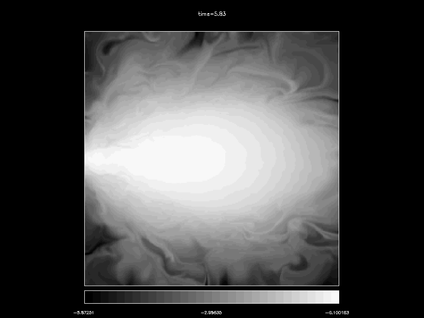
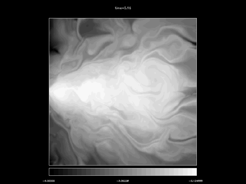
Figure 5: Snapshots of the density logarithm in the self-gravitating model A2b (left panel) after 5.85 orbits at the initial pressure maximum and in the non self-gravitating model B (right panel) after 5.94 orbits. The self-gravitating torus has developed an inner Keplerian thin disc fed by an outer thick ring. The zero mass model shows a much less coherent structure, with large density fluctuations, and an approximately constant $H/r$ value.

In Figure 3 (left panel), we show the contours of the density distribution in the $(r-z)$ plane for model A2b at time $5.85$, just after turbulence has set in (cf also the left hand side of Figure 5). The initial torus has developed a dual structure composed of an inner thin disc, through which matter is accreted toward the central point mass, and an outer thick torus that feeds the inner disc. The gravitational potential is dominated by the central star in the inner thin disc, and by self-gravity in the outer thick disc. Figure 3 (right panel), shows that the rotation profiles are consistent with this. We plot the angular momentum profile in the equatorial plane of the disc averaged between orbits $5.05$ and $7$ (solid line). The inner disc is in Keplerian rotation around the central mass (dashed line) out to a radius of $0.4$. Beyond this point, a power law with exponent $0.9$ can be fit to the profile (dotted line), close to the constant $V_{\phi}$ profile of a fully self-gravitating Mestel disc (Binney & Tremaine, 1987; Bertin & Lodato, 1999).

In our disk model, $Q_{min}\sim 0.3$, which means that the smallest unstable wavelength $\lambda_{min}$ is roughly equal to $0.5$, which is smaller than the radial extent of the disk. In spite of the presence of these unstable wavelengths, self-gravity does not seem to be able to enhance local MRI density inhomogeneities.

3.2 Comparison with zero mass tori

Since they have very different structures, the question of how to draw a comparison between self-gravitating and non-self-gravitating runs is not completely straightforward. For example, neither choosing similar initial $\beta$ values nor saturated $\alpha$ values is satisfactory, since it greatly over emphasizes the (rather minimal) role of gas pressure. More revealing is the value of the stress compared with the rotational energy it is attempting to disturb. Accordingly, we define the ratio $R$ by:

$$R=\frac{\langle T^{Max}_{r\phi}\rangle+\langle T^{Rey}_{r\phi}\rangle}{\langle\rho v_{\phi}^{2}\rangle}\,.$$ (18)

By design, $\langle\rho v_{\phi}^{2}\rangle$ are similar in each of the initial models. Consequently, the value of $R$ will be determined by the level of angular momentum transport. As noted, the MRI growth rates will be nearly the same in the two models, because the angular velocity profiles are similar. We have found that an initial $\langle\beta\rangle$ value of 200 in our zero mass model gives a very similar evolutionary $R$ profile to our high resolution model A2b (see fig. 4). We refer to this zero mass run as model B.

Density displays for model A2b after $5.85$ orbits (left panel) and for model B after $5.94$ orbits (right panel) are shown in figure 5. The scale is logarithmic. Both cases are fully turbulent, but the difference is visually striking: model A2b clearly has a much more coherent internal structure than does model B. An FFT of the radial fluctuations in the disc midplanes shows that on a scale of $\sim 1/15$ of the grid size, the non self-gravitating amplitudes are a factor of $\sim 2$ larger than those of the self-gravitating run. This is comparable to what is seen in the lower resolution model A2a. It is possible that the long range nature of Newtonian gravitational forces is responsible for the higher degree of coherence seen in self-gravitating discs compared with zero mass discs. It should be noted, however, that self-gravitating models also require a higher equilibrium pressure, and this tends to enhance the size of coherent structures, as well (Sano et al., 2004).

3.3 Effect of the variation of the field strength

Finally, we consider the effect of the initial field strength on the evolution of the massive torus. We compare model A1 ($\langle\beta\rangle=400$) and A2b ($\langle\beta\rangle=1500$). Everything else is kept the same.

The Maxwell stress history is shown in figure 6. $\langle T_{r\phi}^{Max}\rangle$ is larger in model A1 (dashed line) during the whole simulation. It exceeds the value reached in model A2b (solid line) by a factor of about 3 at the maximum stress level. A larger stress results in a larger mass accretion rate in model A1 compared with model A2b. This behaviour of retaining a memory of the initial field strength is qualitatively similar to what has been found before in 2D simulations of zero mass discs (Stone & Pringle, 2001).

Figure 7 shows the state of model A1 after $5.83$ orbits (it should be compared with model A2b in figure 3). Density contours are presented on the left side and the angular momentum radial profile on the right side. The density structure at this stage is more disturbed than in model A2b, showing a larger level of MHD turbulence. However, the disc naturally adopts the same radial distribution of angular momentum as in model A2b: Keplerian in the inside, and “Mestellian” in the outer parts. Note that the transition radius is larger in model A1 than in model A2b. This is because the mass accretion rate is larger in the former and the central point mass consequently greater; self-gravity is less important in this case.

To conclude: while the simulations retain a memory of their initial field strength and show different levels of turbulent stress, both tend toward a final state of an inner Keplerian rotational profile and an outer Mestel-like self-gravitating rotation profile.

4 Discussion and Conclusion

In this paper, we have investigated the qualitative behaviour of the MRI in a self-gravitating tori. We performed 2D numerical simulations of the evolution of weakly magnetized, massive tori. The simulations are constructed so that no gravitational instability develops. As a consequence, self-gravity cannot transport angular momentum outward as in 3D. The torus evolves only because of the effect of the MRI induced MHD turbulence. We found that the MRI behaves in these massive discs qualitatively much like it does in the non self-gravitating disc, though there are differences in the density response (see below).

Self-gravitating magnetized tori evolve toward a structure composed of two parts: an inner thin disc in Keplerian rotation around a central mass, fed by an outer more massive thick torus. The gravitational potential in the torus is dominated by the self-gravitating component of the potential and it is no longer Keplerian. Rather, its velocity profile is approximately that of a Mestel disc, $v_{\phi}={\rm constant}$. This steepening of the specific angular momentum profile at large radii has been seen in VLBI observations of water maser emission in the active galactic nuclei NGC 1068 (Greenhill et al., 1996). In this case, the best fit to the angular momentum profile is $j\propto r^{0.69}$. Although we don’t find exactly the same radial profile, our result is quite close (we obtain $j\propto r^{0.9}$). The disagreement probably comes from the fact that the mass ratio between the central object and the disk in our simulation and in the actual system are different. In the latter, the disk mass is comparable to the central black hole mass (Lodato & Bertin, 2003). In our case, the mass of the disk is twice the mass of the central object, thereby giving larger rotational velocities and a steeper profile.

In an attempt to highlight the difference between self-gravitating and zero mass discs, we compared two such simulations with similar density and rotation profiles, and similar evolutionary histories of their stress tensors. The appearance of the zero mass disc was, however, considerably more disrupted than that of the self-gravitating disc. The former showed large density fluctuations, while the latter maintained a much more globally coherent structure. One might have expected to see density fluctuations locally enhanced because of the presence of self-gravity. On the contrary, this is the global nature of the potential that seems to be more important in affecting the evolution of the disk: in this regime, it smoothes the effect of the turbulence and gives more coherence to the disk.

Of course, there are imporant limitations to this study imposed by axisymmetry. First, the turbulence is not sustainable because of the anti-dynamo theorem: it decays and the two component Kepler-Mestel structure described above evolves imperceptively after a few dynamical timescales. Follow-up 3D calculations are essential to track the evolution of this two-component disc. Even more importantly, 3D calculations will allow the development of nonaxisymmetric structure, and allow a full investigation of the interaction between MHD turbulence and spiral structure gravitational instabilities. This important problem is the subject of the companion paper following this one.

Figure 1: Density contour in the (r-z) plane of 2 tori whose density field has been computed using the SCF method. The maximum density is $\rho_{max}=1$ and there are 5 contour levels with $\rho=10^{-4},0.1,0.5,0.7$ and $0.9$. The calculations are done with $P\propto\rho^{\gamma}$ with $\gamma=5/3$ and $\Omega\propto r^{-q}$ with $q=1.68$. The left hand side model has a central mass whose mass is half that of the torus, and the right hand side model is a zero mass torus.

Figure 2: Maxwell (solid line) and Reynolds (dashed line) stress history in model A2b. The time is measured in units of the initial orbital time at pressure maximum. The initial growth of the MRI is shown by the rapid buildup of the Maxwell stress, and is followed by a turbulent phase during which the Maxwell stress decays because of the anti-dynamo theorem. In agreement with simulations of non self-gravitating discs, the Reynolds stress tensor is always smaller than the Maxwell stress.

Figure 3: The left hand side panel shows the density contour in the (r-z) plane for model A2b after 5.85 orbits, normalized by the maximum density. There are 7 levels: $\rho/\rho_{max}=0.01,0.1,0.2,0.3,0.4,0.5,0.7$. The right panel shows the specific angular momentum profile (solid line) for the same model averaged between orbits $5.05$ and $7$. The dashed line shows the Keplerian profile expected for the central mass, while the dotted line is a fit of the outer part of the disc, with $l\propto r^{0.9}$.

Model	$M_{c}/M_{d}$	H/2	$\langle\beta\rangle$	resolution
T	0.5	0.6	-	$128\times 128$
A1	0.5	0.6	400	$256\times 256$
A2a	0.5	0.6	1500	$128\times 128$
A2b	0.5	0.6	1500	$256\times 256$
B	$\infty$	0.5	200	$256\times 256$

Table 1: Model parameters. Column $2$ gives the ratio between the central mass $M_{c}$ and the disc mass $M_{d}$. Column $3$ gives the height of the computational domain (extending between $-H/2$ and $H/2$). Column $4$ gives the ratio of the volume averaged initial values of the thermal and magnetic pressure. Column $5$ gives the resolution of the run.

Figure 4: Comparison between the time evolution of $R$ (See text) in models A2b (solid line) and B (dashed line). The values obtained are very close in both runs throughout the simulations.

Figure 6: Comparison between the time history of the Maxwell stress tensor in model A2a (solid line) and in model A1 (dashed line).

Figure 7: Same as figure 3, but for model A1. The left hand side plot is taken after 4.5 orbits at the initial maximum pressure location and the angular momentum shown on the right hand side was averaged between the orbits 3.88 and 5.05.

References

- Abramowitz & Stegun (1965) Abramowitz, M., & Stegun, I. 1965, Handbook of Mathematical Functions with Formulas, Graphs, and Mathematical Tables (New York: Dover)
- Balbus & Hawley (1991) Balbus, S., & Hawley, J. 1991, ApJ, 376, 214
- Balbus & Hawley (1998) —. 1998, Rev.Mod.Phys., 70, 1
- Bertin & Lodato (1999) Bertin, G., & Lodato, G. 1999, A&A, 350, 694
- Binney & Tremaine (1987) Binney, J., & Tremaine, S. 1987, Galactic dynamics (Princeton University Press)
- Boss (1997) Boss, A. P. 1997, Science, 276, 1836
- Boss (1998) —. 1998, ApJ, 503, 923
- Boss & Myhill (1995) Boss, A. P., & Myhill, E. A. 1995, Comput. Phys. Commun., 89, 59
- Cassen & Moosman (1981) Cassen, P., & Moosman, A. 1981, Icarus, 48, 353
- Cohl & Tohline (1999) Cohl, H. S., & Tohline, J. E. 1999, ApJ, 527, 86
- Evans & Hawley (1988) Evans, C., & Hawley, J. 1988, ApJ, 33, 659
- Greenhill et al. (1996) Greenhill, L., Gwinn, C., Antonucci, R., & Barvainis, R. 1996, ApJ, 472, L21
- Hachisu (1986) Hachisu, I. 1986, ApJS, 62, 461
- Hawley (2000) Hawley, J. F. 2000, ApJ, 528, 462
- Hirsch (1988) Hirsch, C. 1988, Numerical Computation of Internal and External Flows - Volume 1, Fundamentals of Numerical Discretization. (Wiley)
- Huré (2002) Huré, J.-M. 2002, A&A, 395, L21
- Laughlin et al. (1997) Laughlin, G., Korchagin, V., & Adams, F. 1997, ApJ, 477, 410
- Lodato & Bertin (2003) Lodato, G., & Bertin, G. 2003, A&A, 398, 517
- Mayer et al. (2002) Mayer, L., Quinn, T., Wadsley, J., & Stadel, J. 2002, Science, 298, 1756
- Muller & Steinmetz (1995) Muller, E., & Steinmetz. 1995, Comput. Phys. Commun., 89, 45
- Pickett et al. (2000a) Pickett, B., Cassen, P., Durisen, R., & Link, R. 2000a, ApJ, 529, 1034
- Pickett et al. (2000b) Pickett, B., Durisen, R., Cassen, P., & Mejia, A. 2000b, ApJ, 540, L95
- Pickett et al. (2003) Pickett, B., Mejia, A., Durisen, R., Cassen, P., Berry, D., & Link, R. 2003, ApJ, 590, 1060
- Sano et al. (2004) Sano, T., Inutsuka, S., Turner, N. J., & Stone, J. M. 2004, ApJ, 605, 321
- Shakura & Sunyaev (1973) Shakura, N. I., & Sunyaev, R. A. 1973, A&A, 24, 337
- Stone & Pringle (2001) Stone, J., & Pringle, J. 2001, MNRAS, 322, 461
- Stone & Norman (1992a) Stone, J. M., & Norman, M. L. 1992a, ApJS, 80, 753
- Stone & Norman (1992b) —. 1992b, ApJS, 80, 791
- Tohline & Hachisu (1990) Tohline, J., & Hachisu, I. 1990, ApJ, 361, 394
- Yorke & Kaisig (1995) Yorke, W., & Kaisig, M. 1995, Comput. Phys. Commun., 89, 29