The Chemical Enrichment History of the Fornax Dwarf Spheroidal Galaxy from the Infrared Calcium Triplet

Abstract

Near infrared spectra were obtained for 117 red giants in the Fornax dwarf spheroidal galaxy with the FORS1 spectrograph on the VLT, in order to study the metallicity distribution of the stars and to lift the age-metallicity degeneracy of the red giant branch (RGB) in the color-magnitude diagram (CMD). Metallicities are derived from the equivalent widths of the infrared Calcium triplet lines at 8498, 8542, and 8662 Å, calibrated with data from globular clusters, the open cluster M67 and the LMC. For a substantial portion of the sample, the strength of the Calcium triplet is unexpectedly high, clearly indicating that the main stellar population of Fornax is significantly more metal-rich than could be inferred from the position of its RGB in the CMD. We show that the relative narrowness of the RGB in Fornax is caused by the superposition of stars of very different ages and metallicities.

The region of parameter space occupied by the most metal-rich red giants in Fornax –young, metal-rich and luminous– is not covered by any of the calibrating clusters, which introduces uncertainty in the high end of the metallicity scale. Using published theoretical calculations of CaII triplet equivalent widths, we have investigated their sensitivity to luminosity, age, and metallicity. The correlation between absolute I magnitude and CaII strength appears to be only slightly affected by age variations, and we have used it to estimate the metallicities of the Fornax stars.

The metallicity distribution in Fornax is centered at [Fe/H]=$-$0.9, with a metal-poor tail extending to [Fe/H]$\simeq-$2. While the distribution to higher metallicities is less well determined by our observations, the comparison with LMC data indicates that it extends to [Fe/H]$\sim-$0.4. By comparing the metallicities of the stars with their positions in the CMD, we have derived the complex age-metallicity relation of Fornax. In the first few Gyr, the metal abundance rose to [Fe/H]$\sim-$1.0 dex. The enrichment accelerated in the past $\sim$ 1-4 Gyr to reach [Fe/H]$\sim-$0.4 dex. More than half the sample is constituted of star younger than $\sim$ 4 Gyr, thus indicating sustained recent star formation in Fornax. These results are briefly compared to the theoretical predictions on the evolution of dwarf galaxies. They indicate that the capacity of dwarf spheroidal galaxies to retain the heavy elements that they produce is larger than expected.

1 Introduction

During the last decade, the deep, wide field color-magnitude diagram (CMD) studies and spectroscopy of the dwarf spheroidal (dSph) satellites of the Milky Way have beautifully confirmed early hints on the fact that these galaxies had experienced more than one episode of star formation and nucleosynthesis (Zinn 1981, and references therein). Indeed, we find almost every imaginable evolutionary history in this sample of galaxies, from the extreme case of Leo I, which has formed over 80% of its stars in the second half of the life of the Universe (Gallart et al. 1999), to intermediate cases like Carina (Smecker-Hane et al. 1996; Hurley-Keller, Mateo & Nemec 1998) and Fornax (Stetson, Hesser & Smecker-Hane 1998; Buonanno et al. 1999), with prominent intermediate-age populations, to predominantly old ($\simeq$ 10 Gyr old) systems like Sculptor (Hurley-Keller, Mateo & Grebel 1999), Draco (Aparicio, Carrera & Martínez-Delgado 2001), Ursa Minor (Mighell & Burke 1999; Carrera et al. 2002) and Leo II (Mighell & Rich 1996).

The very extended star formation history (SFH) in several of these galaxies seems to be independent of their total mass: Carina and Leo I are among the least massive dSph in the Milky Way system, with virial masses around $2\times 10^{7}M\odot$, while Fornax is the most massive one, with $7\times 10^{7}M\odot$, see Mateo (1998). Their metal content, however, is directly related to their total luminosity, and presumably, to their total mass (Caldwell et al. 1998 and references therein): Leo I and Carina have low metallicities (Gallart et al. 1999; Smecker-Hane et al. 1999), while Fornax seems to have a relatively high metallicity and a large metallicity dispersion (Saviane et al. 2000; Tolstoy et al. 2001; and much more prominently in this paper). The metal content, therefore, seems to be not as much related to the SFH than to the ability of these systems to retain the produced metals, which may have to do with the effect of SNe on the interstellar medium and the depths of their potential wells (e.g., Mac-Low & Ferrara 1999; Ferrara & Tolstoy 2000).

The nearest galaxies offer an excellent opportunity to test these correlations and their theoretical interpretation, since their SFH can be derived with great accuracy from deep CMDs, their masses can be calculated from the velocity dispersion of their stars, and the metallicities and metallicity distribution can be obtained from spectroscopy of their individual stars. It is important to emphasize the need to replace the common technique of inferring the mean and the dispersion in metal abundance from the mean color and color spread of the RGB in the CMD under the assumption that the stars in these galaxies are very old. Because of the age-metallicity degeneracy in the position on the RGB, this method can lead to significant errors if the galaxies contain, as some do, sizable populations of intermediate-aged stars. Spectroscopic metallicity determinations exist for a small sample of the nearest dSph using the Ca II  triplet and other metallicity indicators in low dispersion spectra (Draco: Lehnert et al. 1992, and references therein; Winnick & Zinn, in prep.; Sextans: Da Costa et al. 1991; Suntzeff et al. 1993; Carina: Smecker-Hane et al. 1999; Sculptor: Tolstoy et al. 2001; Fornax: Tolstoy et al. 2001). All of the studies that have observed more than a few stars have discovered that substantial metallicity dispersions are present, even though the mean metallicity of each of these low-mass systems is low. High dispersion abundance determinations of a number of elements require necessarily an 8m-class telescope, and exist for a few stars in the nearest northern dSph, namely Draco, UMi and Sextans, for which Keck HIRES spectroscopy has been possible (Shetrone, Côté & Sargent 2001; Shetrone, Bolte & Stetson 1998) and in the nearest southern dSph, Sculptor, Fornax, Carina and Leo I, using UVES at the VLT (Shetrone et al. 2003; Tolstoy et al. 2003). These studies have measured just a few stars in each galaxy, and confirm the low resolution spectroscopy results in the cases where there is overlap, in terms of mean metallicity and existence of a dispersion in metallicity. Among the new information that they provide is the abundance patterns among the dSph galaxies, which are quite uniform, indicating similar nucleosynthetic histories and presumably similar IMF. The $[\alpha/Fe]$ element ratios are however in general lower in the dSph than in the Galactic Halo, for the same range of metallicity.

In this paper we present spectroscopy and metal abundances for a large number of stars in the Fornax dSph galaxy. Fornax is a particularly interesting galaxy in the context of the study of chemical enrichment processes in dSph galaxies, since it seems to be among the few Milky Way dSph satellites (the other outstanding one being Sagittarius, see Layden & Sarajedini 2000 and references therein) that has been able to retain substantial amounts of metals during its evolution, as hinted by the width of its RGB (Saviane et al. 2000) and confirmed and shown to be even more extreme by the spectroscopic work presented in this paper. Tamura, Hirashita & Takeuchi (2001) consider it as the only galaxy in our immediate neighborhood with properties comparable to the more massive dwarf elliptical (dE) Andromeda companions. Fornax is indeed one of the most massive of the Milky Way satellite dSph galaxies, with total mass $6.8\times 10^{7}M\odot$ (Mateo 1998), as inferred from the central velocity dispersion of its stars (Mateo et al. 1991), and it is one of the two (again with Sagittarius) containing its own system of globular clusters. The existing deep CMDs (Stetson et al. 1998; Buonanno et al. 1999; Saviane et al. 2000) show a blue horizontal-branch and a well populated red-clump indicating a substantial population of old and intermediate-age stars respectively, and a relatively bright main sequence which must contain stars as young as a few hundred million years. Particularly puzzling is the fact that no HI gas is found in deep VLA observations near the center of the galaxy (Young 1999), where the youngest stars are found. The current data cannot definitely exclude, however, the presence of HI in the outer parts of Fornax, where it may reside if it was ejected by the last event of star formation.

To understand in more detail the evolution of Fornax, one would like to measure its age-metallicity relation (AMR) and its SFH. This can be done if the age-metallicity degeneracy of the RGB and other features of the CMD can be broken by observations that yield the abundances of the stars independently of their ages. The infrared Ca II  triplet has been shown to be a useful metallicity indicator for metal-poor stars (see e. g. Rutledge et al. 1997a, hereafter RHS, and references therein). While most previous investigations that have used the infrared Ca II  triplet as a metallicity indicator have worked on globular clusters or other very old star systems, a few have collected observations of red giants in significantly younger stellar populations and have shown that the metallicities obtained in this way are consistent with other estimates (Olszewski et al. 1991; Suntzeff et al. 1992; Da Costa & Hatzidimitriou 1998). This previous work motivated us to secure spectra at the Ca II lines of a sample of 117 stars in Fornax that lie near the tip of its RGB. We suspected that this sample would contain stars covering nearly the entire ranges in age and in metallicity. To demonstrate that these observations are not compromised by an age-metallicity degeneracy, we discuss the sensitivity of Ca II strength to age and metallicity variations using the theoretical calculations by Jorgensen, Carlsson & Johnson (1992), and we show that the observations of star clusters are consistent with the theoretical expectations. We then derive the metallicities of the Fornax stars from a new calibration of the Ca II triplet, estimate the AMR and discuss the SFH of this galaxy.

2 Observations and Reductions

The observations were obtained on the night of 1st December 1999, using the FORS1 instrument installed on the Cassegrain focus of the UT1 telescope (first 8.2-m unit of the ESO Very Large Telescope) at Paranal, Chile. FORS1 is a low-dispersion spectrograph that allows the simultaneous spectroscopy of up to 19 objects in a 6.8’x6.8’ field of view through a system of adjustable slitlets. Grism GRIS-600I+15 was used with order separation filter OG590+72, resulting in a central wavelength of 7940 Å, a dispersion of 1.06 Å  per pixel (44 Å/mm), and a resolution of $\sim$ 1530. The spectral range covered was in general 7000-9000 Å, with variations depending on the exact position of the slitlet in the field. In positioning the slitlets, we ensured that the whole spectral region of interest to measure the Ca II  triplet feature was always covered. Calibration exposures were taken for each setup in the morning following the observations with a Ne-Ar lamp. The excellent seeing conditions during the observations –most of the time below 0.8” seeing– allowed us to use slitlet widths of 0.7 arcsec.

Seven fields were observed in Fornax, with an average of 17 targets per field. For each field, two 20-minute exposures were acquired on two positions offset vertically by about 3 arcsec ($\sim$10 pixels). This procedure allows the direct subtraction of the sky from the unextracted spectra, in spectroscopic analogy to the method widely used in infrared photometry. The method is a simplified version of the ”va-et- vient” procedure presented by Cuillandre et al. (1994). It is much more effective at removing the night sky emission lines than the conventional method of interpolating between sky spectra that are recorded on either side of the object spectrum. Short exposures were also acquired on selected red giants of three nearby globular clusters, NGC 2298, NGC 3201 and NGC 7099=M 30, for the purpose of the metallicity calibration. A single exposure with an exposure time of 2-5 minutes was obtained for each cluster. Because red giants near the tip of the RGB are much less dense in the plane of the sky in the globular clusters than in Fornax, only a small fraction of the slitlets could be used in the cluster exposures.

2.1 Target selection

The program targets were selected in the upper part of the RGB in Fornax within the central 11 arcmin of the galaxy. We used the $B$ and $R$ band photometry of Stetson et al. (1998) for this selection. For the purpose of the target selection only, the $I$ magnitude was extrapolated from the $B$ and $R$ using a relation fitting globular cluster data: $I\simeq R-\frac{1}{2}(B-R)+0.35$. The $V$ and $I$ values used later in the article and listed in Table 2 are from the new photometry of Fornax by Gallart et al. (in prep.). The targets were selected with linear limits on color and magnitude encompassing all the upper part of the Fornax RGB down to $I=18.35$: $16.60<I<18.35$ and $-3.24(B-R)+23.02<I<-2.61(B-R)+23.52$. The $I$ magnitude was used to define the selection because it corresponds to the wavelengths of the Ca II  triplet region. The color selection limits were designed in order to include the whole width of the Fornax RGB, including potential outliers on the blue side, while excluding regions obviously dominated by field stars.

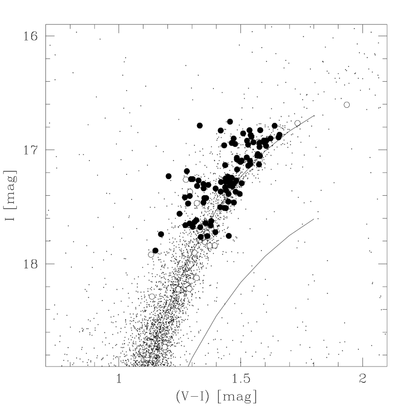
Figure 2: Upper CMD of Fornax. Large dots indicate the measured targets and open symbols denote likely non-members and objects removed from the final analysis by the S/N criteria. The sequences of the globular clusters at [Fe/H]=$-$ 1.1 and [Fe/H]=$-$ 0.7 (from Saviane & Rosenberg 1999) are also indicated.

This selection produced 2534 potential targets. The actual targets were picked according to their position in the field of the instrument, in order to fill optimally the 19 slitlets available for multi-object spectroscopy on FORS1. The position of all observed targets is shown on Fig. 1 on the plane of the sky and Fig. 2 in the CMD.

While age, metallicity or kinematic criteria were not used in the selection, some age and metallicity selection is however implicit in the color and magnitude limits. The upper part of the RGB is not a totally representative sample of a given stellar population. In Section 3.2 we attempt to infer the metallicity distribution of the complete population from the distribution of our sample.

2.2 Spectra reduction

The spectra were reduced using the noao packages twodspec.apextract and onedpec in IRAF. The procedure was somewhat different for the program stars, for which two offset frames were obtained, and for the calibrating globular clusters, for which only one frame of short exposure was obtained.

Fornax frames

The frames were flat-fielded with lamp flatfields taken after the night with the same spectrograph and slitlet configuration than the program frames. A variable width at the side of each slitlet was removed to avoid reflections. In three cases, namely targets 217, 302 and 714, this procedure removes part of the spectra.

Cosmic rays were removed with the IRAF task cosmicrays, and the two offset frames were subtracted to obtain an image with a positive and negative spectrum, some 10 pixel apart, for each slitlet. The positive and negative spectra were extracted with a width of 8 pixels and calibrated in wavelength using Ne-Ar lamp exposures taken at the end of the night and the spectral line wavelengths listed in the FORS user manual (In the case of frame 5, the wavelength calibration exposure was corrupted and re-done several weeks after the observation). The residual wavelength scatter was smaller than 0.1 Å. Attention was given to the stability of the calibration between 8400 and 8700Å –the region of the Ca II triplet lines– allowing for possible non-linear distortions on the edges of the spectral range. The two offset, wavelength calibrated spectra, one positive and one negative, were then subtracted to produce the final spectrum.

This procedure allows a very efficient removal of the sky background. Most of the sky cancels out in the direct subtraction of the two images, independently of the variations in pixel response. It is therefore unaffected by the errors in the flat-fielding. The only sky light left in the subtracted images is that due to variation of its intensity between the two 20-minutes exposures, which is removed when the two extracted, wavelength calibrated spectra are subtracted again. An example of the raw, sky and final object spectra is given in Fig. 3.

The reduction procedure was checked by extracting the spectra of all the objects of frame 4 by two authors independently, using slightly different parameters. The resulting spectra were essentially identical. Varying the extraction width between 1 and 10 pixels was also tested on frame 4, and 8 pixels was judged to be a reasonable value to apply to all spectra. While marginally better results could have been obtained by tailoring the extraction width to each spectrum, this would have introduced a subjective element regarding what constituted a “bad feature”. Consequently, we used the same extraction width for all spectra.

Globular cluster calibration frames

Only a single exposure was obtained of the globular cluster red giants that serve to calibrate the pseudo-equivalent widths, because they are much brighter than the sky background. Their spectra were extracted after de-biasing and flat-fielding. The sky was removed by a linear fit to the background perpendicular to the direction of the dispersion.

We observed several RGB stars in three globular clusters, NGC 2298, NGC 3201 and NGC 7099, which were selected from the photometry of Alcaino & Lillier (1986), Lee (1977) and Dickens (1972) respectively. We chose preferentially stars whose Ca II  triplet equivalent widths were measured by Rutledge et al. (1997a, hereafter RHS). The exposure times for the clusters were 300 sec, 180 sec and 120 sec respectively. Table 1 lists the information on the measured stars. The Star ID and the B, V magnitudes are taken from the above references. The equivalent widths of the three Ca II lines and their sigma are listed in columns 5–10. The combined equivalent widths as measured in this work and its sigma are listed in columns 11-12, and the same information as measured by RHS is listed in columns 13-14. Stars DP91, DP23, and DP24 in NGC 7099 were not observed by RHS, and the values listed are the result of transforming the observations of Suntzeff et al. (1993) to the RHS scale using the equation given by RHS.

2.3 Radial velocities

Radial velocities were obtained by fitting each of the three Ca II  lines with a Gaussian profile in IRAF. Velocities were then computed using the measured line centers and the known lab wavelengths (taken from RHS). Whenever possible, all three lines were used to compute the final averaged velocity for an individual star.

The low resolution of the spectra limits the usefulness of the radial velocity to the identification of clear outliers as likely non-members of Fornax, without allowing a more detailed kinematical study. Objects 109, 214 and 418 have discordant velocities and are suspected non-members. The velocity of 216 is also discordant, but the spectrum is too noisy for the indication to be reliable. In the following analysis, the first three objects are excluded, while the fourth falls much below our spectral quality criteria and is excluded anyway (Par. 2.4).

2.4 Ca II equivalent width

Pseudo equivalent widths were calculated from the spectra using passbands in and around the Ca II  triplet lines. To place our measurements on the system of RHS, we followed closely their prescription for measuring the pseudo-equivalent widths. We used the same functional form, the Moffat function of exponent 2.5, for fitting the lines and the same wavelength intervals for continuum passbands. For the measurement of the combined equivalent width we used their definition of the weighted sum of the widths, $\Sigma$Ca, which they defined as $\Sigma$Ca$=0.5w1+w2+0.6w3$, where $w1,w2$ and $w3$ are the equivalent widths of individual Calcium lines ($\lambda$ 8498, 8542, 8662Å, respectively). We observed 19 red giants in the globular clusters NGC 2298, NGC 3201, and NGC 7099 for which values of $\Sigma$Ca  were measured by RHS or could be transformed to their system (see Table 1). The mean difference in the sense ours minus theirs between the values of $\Sigma$Ca is $0.04$, with a standard deviation of 0.11. Since these deviations are small compared to the average measuring errors (0.16 and 0.10 for our and RHS values, respectively), no corrections appear necessary to put our measurements on the RHS system.

As a consistency check, the equivalent width were also calculated by fitting a Gaussian profile on the spectra with the ”splot” task in IRAF, after the spectra continuum were flattened by division with a 6-th order polynomial. The Gaussian and Moffatian values were found to be in excellent agreement. A regression between the equivalent widths calculated with the two methods gives $\Sigma$Ca${}_{Moff}=1.005$$\Sigma$Ca${}_{Gauss}+0.014$Å, $\sigma$=0.12 Å. The passband value was adopted except when there was a visible spike in the continuum near the Calcium lines. In that case the Gaussian fit was preferred. In the case of frame 5, only the Gaussian values were computed. Table 2 indicates when Gaussian fitting was chosen.

The signal-to-noise ratio per pixel was evaluated by computing the dispersion of the normalized background in three different wavelength intervals around the Ca II  lines : $\lambda=8390-8489$ Å, $8555-8650$ Å, $8695-8794$ Å. Spectra were included in the analysis when the signal-to-noise ratio in these intervals was higher than 20 (metallicities are nevertheless given in Table 2 down to a signal-to-noise ratio of 14). Note that this criteria, which takes into account the noise on the side of the Ca II  lines only, will not produce any bias at selectively eliminating spectra of lower metallicity stars. Stars rejected by this criteria or for other reasons mentioned in the notes are shown as open dots in Figure 2 (23 out of 118 stars). In Figure 4, three sample spectra are shown. The final uncertainty of the combined Ca II  equivalent widths is in the range 3-6% for our objects.

3 Calibration and results

3.1 Metallicity calibration of the Ca II  triplet

As discussed in the introduction, previous studies have shown that the strengths of the infrared Ca II triplet lines can be used as a metallicity indicator for old, metal-poor stars, such as the ones in globular clusters. It is less clear that these lines provide an accurate metallicity ranking for red giants of near solar composition and for ones spanning a wide range in age. Since Fornax contains red giants with these properties in addition to very old, metal-poor ones, it is imperative that we investigate the behavior of the Ca II lines in some detail.

In the Appendix, we use theoretical calculations of Ca II  line strength as a function of effective temperature and log g, together with theoretical isochrones, to investigate the sensitivity of the CaII lines to age and metallicity.

Most previous investigations that used $\Sigma$Ca as a metallicity indicator have plotted it against V-V(HB) because this quantity is independent of the reddening and the distance modulus of the system. This quantity works fine for very old stellar populations that have well-defined horizontal branches and small or virtually non-existent internal metallicity spreads, such as most globular clusters. The metallicity calibration of the plot of $\Sigma$Ca vs. V-V(HB) corrects implicitly for the systematic variation in HB luminosity with metallicity. It is much less clear that V-V(HB) is a useful parameter for a galaxy like Fornax that possesses wide ranges in age and metallicity. In the case of an intermediate-age star cluster, one can make the necessary correction to V-V(HB) because the ages of the red giants are known (e.g. Da Costa & Hatzidimitriou 1998). But in Fornax, because the age of an individual red giant cannot be determined, one does not know if its V-V(HB) should be corrected for age.

Since the distance modulus of Fornax is well determined and differential reddening is negligible, it is possible to determine unambiguously the absolute magnitude of every star. If plots of $\Sigma$Ca against absolute magnitude yield a metallicity ranking that is reasonably insensitive to age, then it does not matter that the ages of the red giants span a large range and that the ages of individual stars cannot be determined.

Fig. 5 shows the Fornax and cluster data in the projections relevant to the metallicity calibration. The discussion in the Appendix indicates that:

i) When clusters of different ages are considered, indicators primarily sensitive to gravity, like absolute magnitude, are expected to be much better for the $\Sigma$Ca calibration than indicators sensitive primarily to temperature, for example (V-I). The relatively young and metal-rich open cluster M11 provides an important check on the age sensitivity. Suntzeff et al. (1992, 1993) measured the infrared Ca II  lines in the spectra of 21 red giants in M11, which we have transformed to $\Sigma$Ca using the transformation equations in RHS. M11 can be compared to the older, similarly metal-rich calibrating cluster M67. Fig. 5 confirms the importance of gravity effects on the Ca II  triplet equivalent width. M11 and M67 occupy widely different positions in the (V-I) vs $\Sigma$Ca plot and the $M_{I}$ vs (V-I) plot, even though their metallicity is similar, because their age difference causes large gravity differences at a given temperature.

ii) An abundance calibration of the Ca II  triplet using the $M_{I}$ magnitude is somewhat less sensitive to age than one using $M_{V}$. Our calibration of $W_{0}$ (defined below as $\Sigma$Ca at M_I=0) with [Fe/H] on the Carretta & Gratton scale (see below) yields a mean [Fe/H] of +0.02 $\pm$ 0.03 for M11, which suggests a remarkably low sensitivity of the $\Sigma$Ca - $M_{I}$ diagram to age. We have also derived a calibration using $M_{V}$ instead of $M_{I}$. This calibration yields a mean [Fe/H] of $-0.21\pm 0.03$ for M11.

For these reasons, in the following analysis, we derive a calibration based on $M_{I}$ because it should produce more accurate results for the youngest stars in Fornax. It is very important to emphasize, however, that the fairly good results obtained for M11 and M67 do not guarantee that the age effect is negligible in the case of the most metal-rich stars in Fornax. These stars lie in a region of parameter space that is not covered by the calibrators (i. e. bluer than M67, brighter than M11, and younger than globular clusters). In particular, the models tend to predict a curvature of the isometallicity lines in the $M_{I}$ vs. $W$ plane for the brightest and most metal-rich red giants (see Fig. 16 in the Appendix). This curvature is not observed in the relatively low-luminosity M67 data. If present at higher luminosity, it would lead to an age-dependent shift of the derived metallicities for the metal-rich end of the Fornax data. It would also, however, cause a systematic trend in the recovered metallicities as a function of luminosity, a trend that is not observed in our data (see Fig. 6).

In the following paragraphs, we first present a metallicity calibration in the $\Sigma$Ca - M_I plane based on the calibrating clusters, and then discuss how it should be modified for the youngest Fornax stars. Our cluster calibration of the $\Sigma$Ca - M_I relation is based on the observations of Ca II  line strengths in 11 globular clusters and M67 from Olszewski et al. (1991), Armandroff & Da Costa (1991), Suntzeff et al. (1992, 1993), Da Costa & Armandroff (1995) and RHS. When it was necessary, the observed values of W(Ca II) were transformed to $\Sigma$Ca using the equations in RHS. The $I$ photometry of the stars was taken from Da Costa & Armandroff (1990), Ortolani et al. (1990, 1992), Ortolani (priv. comm.), Alcaino & Liller (1986), Alcaino, Liller & Alvarado (1989), Lloyd-Evans (1983) and Janes & Smith (1984). For a minority of the stars, I-band photometry was not available in the literature, and it was necessary to derive approximate values from transformations between (B-V)₀ and (V-I)₀. This was accomplished using stars that had been measured in both colors in the clusters. For the very metal-poor cluster NGC7099, the (B-V)₀ vs (V-I)₀ transformation derived by Zinn & Barnes (1996) was used. The uncertainties introduced by these transformations are small compared to the other sources of error in the calibration. The reddenings and V magnitudes of the horizontal branches of the globular clusters were adopted from either the photometric catalogs or from the 1999-version of the compilation by Harris (1996). The distance moduli of the globular clusters were calculated from the V(HB) values using the M_V(HB) relation calculated by Demarque et al. (2000), which takes into account the HB morphologies of the clusters as well as their [Fe/H]. The apparent distance modulus and reddening of M67 were taken from Twarog et al. (1997).

While the $\Sigma$Ca data for all 12 clusters are well correlated with $M_{I}$, the correlation for three clusters are clearly inferior to the other nine. For one of the three clusters (NGC1851), $\Sigma$Ca was available for only 5 stars that span a relatively small range of $M_{I}$. The other two clusters (NGC6528 & NGC6553) lie in very crowded and heavily reddened fields, which may have produced larger than average errors in line strength and $M_{I}$. The tight sequences produced by the other nine clusters are well approximated by straight lines of nearly the same slope, and there is no firm evidence of systematic change in slope with [Fe/H]. The average slope is $-0.48\pm 0.02$, which is also not far from the values obtained with data for NGC1851, NGC6528 and NGC6553. Following previous investigators, we define a reduced equivalent width ($W_{0}$) to remove the increase in $\Sigma$Ca with increasing luminosity.

$$W_{0}=\Sigma\,Ca+0.48\,M_{I}$$

Note that this $W_{0}$ is $\Sigma$Ca at $M_{I}$=0, and therefore not the same as $W^{\prime}$ at V$-$V(HB)=0 as defined by other authors.

To calibrate $W_{0}$ in terms of [Fe/H], we adopted for eight of the globular clusters the value of [Fe/H] that Carretta & Gratton (1997, CG) and Carretta et al. (2001) measured from high dispersion spectra of red giants. Carretta et al. (2001) consider their measurements of the most metal-rich clusters NGC 6528 and 6553 to be on the same scale as the more metal-poor ones that were measured by CG. For NGC1851 and M2, which were not measured by these teams, we selected the values that RHS obtained from a calibration, on the CG scale, of the plot of V(HB)-V against $\Sigma$Ca. Several studies have shown that M67 has a solar composition within the errors, and we adopted [Fe/H]=0.00 $\pm$ 0.10 from Twarog et al. (1997). Our calibration of $W_{0}$ with [Fe/H] is shown in Figure 7. The solid curve is the expression:

$$[Fe/H]=-2.286+0.057\,W_{0}+0.071\,W_{0}^{2}$$ (1)

which was obtained by the least-square method.

This calibration is valid for the regions of the ($V-I$, $M_{I}$, $\Sigma$Ca) space covered by the calibration clusters. It can be applied directly to the Fornax data below [Fe/H]$\sim-1.2$ dex. However, Figure 5 shows that part of the Fornax data lies outside that region. There is no calibrating cluster that is simultaneously as bright, as blue and with as large $\Sigma$Ca as the metal-richest Fornax targets. The M11 sequence has similar colors and $\Sigma$Ca but that cluster is not populous enough to contain stars as bright as in the Fornax sample. This means that the metallicity determination for the metal-richer part of our sample is not entirely constrained by the cluster calibrators and depends on a linear extrapolation of the $\Sigma$Ca-$W_{0}$ relation of about one magnitude in $M_{I}$. Until calibrators are available in that part of the parameter space, there will remain some uncertainties on the highest [Fe/H] inferred from the Ca II  triplet for the brightest red giants.

The indications given about the extrapolation by the theoretical calculations of the Appendix are ambiguous. On the one hand, the theoretical isometallicity sequences in the $M_{I}$-$\Sigma$Ca plane show very little curvature between $M_{I}=-$2 and $M_{I}=-4$. This would support a linear extrapolation to higher $M_{I}$. However, the theoretical relations also indicate a steeper slope of the isometallicity lines for higher metallicities, whereas the observed cluster data is compatible with a constant slope.

On the observational side, Ca II  triplet data for red giants in the LMC (which are as bright and as blue as the Fornax stars with large Ca II equivalent widths) give a strong indication that the extrapolation of the calibration for high luminosities and high metallicities is not linear in $M_{I}$. The LMC data provide complementary information to extend the calibration to stars younger and brighter than those of the calibrating clusters. Recently, Cole et al. (2000) have collected Ca II  data for an extensive sample of red giants in the LMC. The authors encountered the same difficulties in the high-metallicity end of their sample that we noted above in the case of Fornax. The problem is even bigger for the LMC, because it is on average more metal-rich than Fornax. These authors dealt with the problem by taking M67 out of their calibration altogether, consequently extrapolating the $W^{\prime}$-[Fe/H] relation in metallicity as well as the $\Sigma$Ca-$W^{\prime}$ relation in magnitude. The introduction of M67 in their calibration introduces a shift of the order of 0.4 dex in their most metal-rich objects (their Fig. 6). Fortunately there are other reliable constraints on the metallicity distribution of stars in the LMC, independent of the red giant Ca II measurements. Most studies indicate a typical value of about [Fe/H]$\sim-$0.3 for the mean metallicity of the youngest populations (e.g., Luck et al. 1998 who obtain [Fe/H]$\sim-$0.3 for the mean metallicity of Cepheids; the age-metallicity relation of Pagel & Tautvais̆ienė 1998 that culminates at [Fe/H]$\sim-0.2$ based on observational data listed therein). The LMC Ca II  data of Cole et al. (2000) are compared to the Fornax data on Figure 8. It shows that the LMC Ca II  data does reach the luminosities of our Fornax sample, so that the better-constrained LMC data can be used to check the extension of the Ca II  metallicity calibration to higher luminosities.

We accordingly adapt our calibration for high luminosities by imposing a value of [Fe/H]$=-0.3$ at $W_{0}$=5.5 Å, corresponding to the metal-rich end of the LMC sample. The junction between the two calibrations is fixed at [Fe/H]=$-1.2$ dex, the value where the Fornax red giants start having CMD locations different from the globular clusters. The resulting interpolation has very little curvature and is practically equivalent to the linear formula:

$$[Fe/H]=-2.87+0.47\,W_{0}$$ (2)

This calibration is shown as a dotted line on Figure 7. Calibration (1) is valid up to $M_{I}\sim-2$, while the modified calibration (2) is applicable for $M_{I}$ around $-3$ and brighter, like our Fornax sample.

This procedure, which appears justified at this moment, should be checked by observing luminous red giants in open clusters that span wide ranges in age and composition, and more directly by observing at high dispersion some of the metal-rich red giants in Fornax. We have examined the database of Cenarro et al. (2001b) for open cluster stars that overlap the Fornax stars in luminosity and colour. Only two stars in the cluster NGC 7789 are as luminous as some of the Fornax stars, but these stars are significanlty redder. They do not, therefore, provide a direct test of the calibration technique taht we have applied to Fornax. Note that the discussion in the following sections does not depend strongly on the exact values of the highest metallicities in Fornax, the crucial factor being the presence in the sample of a large number of stars with very high values of $\Sigma$Ca.

To apply the $M_{I}$ calibration to the Fornax data we use E(V$-$I)=0.07 for Fornax, which is the mean value that Buonanno et al. (1998) derived for four globular clusters in Fornax, V(HB)=21.28, the mean V magnitude of the horizontal branch of the same 4 clusters, and M_V(HB)=0.47, from the models of Demarque et al. (2000). These numbers give (m-M)_V=20.81 and (m-M)_I=20.74.

The resulting values of [Fe/H] for our sample are given in Table 2, and the resulting metallicity distribution is displayed in Figure 9. Figure 6 plots the [Fe/H] as a function of $I$ magnitude. As a reminder of the fact that the uncertainty on the calibration is higher for the metal-rich part of the Fornax sample, the values above [Fe/H]=$-0.9$ are rounded off and indicated by a colon (“:”) in Table 2, and the corresponding bins are shaded in Fig 9.

This metallicity distribution is broadly consistent with that of Tolstoy et al. (2001): in both cases, most of the stars in the sample have values in the range $-1.5<[Fe/H]<-0.7$ and, if we consider Poisson error bars in the number of stars with metallicities above and below $[Fe/H]=-1$, the relative number of stars may be compatible. Our sample is, however, centered at significantly higher abundances (67% of stars with $[Fe/H]>-1$, compared to 53% in the Tolstoy et al. sample, and the peak of the distribution is $[Fe/H]=-0.9$ compared to $[Fe/H]=-1.2$ in Tolstoy et al.) These differences may be in part explained by the population selection effects resulting from the different brightness of the two samples: our sample is within $\simeq$1 mag below the tip of the RGB, while the Tolstoy et al. sample is between 1 and 3 mags fainter than the tip. As we will show in the next section, selecting bright red giants may imply a bias towards young ages and, considering a general metallicity law in which metallicity increases with time, higher metallicities. Our results are, in any case, statistically more solid, since we have more than three times the number of stars of Tolstoy et al. (2001). Finally, note the much higher quality of our spectroscopic data, reflected in our much lower error bars that those inferred by Tolstoy et al. (0.23 dex on average vs. 0.09 dex of mean error in our measurements). The difference in the quality of the spectra is also evident if one compares their figure 10 with our figure 4. In their figure 10, Tolstoy et al. show a good spectrum of Fornax, with S/N$\simeq$30, which is comparable in quality to all our spectra. The star to which this spectrum belongs, however, is about 2 magnitudes brighter than the rest of their Fornax sample.

3.2 Inferred metallicity distribution for the whole population

The metallicity distribution of our red giant sample is an indirect reflection of the metallicity distribution of Fornax as a whole, since the brightest red giants are only a specific sub-set of the galaxy. To infer the likely metallicity distribution of the underlying population in Fornax from our data, we computed synthetic CMDs and examined the relation between the ”observed” and ”real” metallicity distribution in these models. The models use the synthetic CMD code ZVAR (described in Gallart et al. 1999) with the Bertelli et al. (1994) generation of Padova stellar evolutionary models, an IMF from Kroupa, Tout & Gilmore (1993) and an input star formation rate and AMR to produce a synthetic population. For a description of these parameters and the way they are used, the reader is referred to Gallart et al. (1999). We used a constant star formation rate and experimented with several AMR. All AMR compatible with our Fornax data produce essentially similar results, and we give below the results for an AMR of z=0.0004 at age=15 Gyr, z=0.002 at age=1.5 Gyr, z=0.008 at age=0 Gyr, with linear interpolation in between (the maximum age for the Padova isochrones that we use is 15 Gyr). On this synthetic population, we then apply our selection criteria (see Section 2.1) and compute how many objects fall in different age and metallicity bins. The results are given in Tables 3 and 4. As the input star formation rate is constant, the distribution of the ages of the selected stars indicates the age bias relative to the underlying population (or, more precisely, to the population of stars with $t_{life}>\tau$, such as K-dwarfs) i.e. the synthetic CMDs indicate that we selected preferentially stars with ages $\leq$ 4 Gyr, by about a factor of a 30%. Consequently, the metallicity distribution of the RGB sample is also different from that of the underlying population. The values in Tables 3 and 4 are used in Section 4 to infer the age and metallicity distributions of the whole population from the distributions of our sample.

3.3 Potential sources of uncertainty

i) Possible differences in [Ca/Fe] between Fornax and the calibrating clusters. The equivalent width of the Ca II  triplet depends on the abundance of Calcium, an $\alpha$-element. Relating it to the [Fe/H] scale therefore requires knowledge of the run of [Ca/Fe] with [Fe/H]. Among the calibrating clusters, there is significant variation in [Ca/Fe] that is not uniquely correlated with [Fe/H]. The globular clusters that make up the calibration below the metallicity of 47 Tuc ([Fe/H]=$-$0.7) have on average [Ca/Fe]$\sim+0.3$ (Carney 1996; Sneden et al. 1997; Gonzalez & Wallerstein 1998; Shetrone & Keane 2000). Three studies of 47 Tuc itself (see Carney’s review) indicate that it has [Ca/Fe]$\sim$ 0.0, as does the open cluster M67 (Tautvais̆ienė et al. 2000). The two globular clusters that are more metal-rich than 47 Tuc, NGC 6528 and NGC 6553 have [Ca/Fe]$\sim$ +0.25, according to Carretta et al. (2001). This result and the measurements of [Fe/H] by these authors yield [Ca/H] values that actually exceed the value obtained by Tautvais̆ienė et al. (2000) for M67, which is surprising because these clusters lie below the M67 sequence in the $M_{I}$-$\Sigma$Ca diagram (see Fig. 5). While this apparent inconsistency may be simply due to observational error, it is important to note that the $M_{I}$-$\Sigma$Ca diagram is not only sensitive to [Ca/H] but also to the values of $Te$ and $\log g$ of the stars evolving on the RGB (see Appendix), which are in turn complex functions of the overall metallicities of the stars and their ages. It is not certain that the values of $W_{0}$ that are derived from the $M_{I}$-$\Sigma$Ca diagram should be more closely correlated with [Ca/H] than with [Fe/H]. Further theoretical modeling of the $M_{I}$-$\Sigma$Ca diagram is urgently needed to clarify this point and to put the question of its age sensitivity on a firmer footing.

The possibility remains that the Fornax stars have so different [Ca/Fe] than our calibrating objects that their positions in the M_I-$\Sigma$Ca diagram in Fig. 5 are not indicative of their metallicities. However, the very recent high dispersion analyses of three red giants in Fornax by Shetrone et al. (2003) suggest that this is not the case. They obtained [Ca/Fe] = +0.23, +0.21, and +0.23 for stars that have [Fe/H]= $-$1.60, $-$1.21 and $-$0.67, respectively. Since these values of [Ca/Fe] are near the mean of our calibrating clusters, we highly doubt that the Fornax stars in our sample have so different [Ca/Fe] values that the $M_{I}$-$\Sigma$Ca diagram produces for them an erroneous ranking by [Fe/H].

ii) AGB stars. Synthetic population simulations (see Section 3.2) indicate that about a quarter of the stars in our sample are probably AGB stars rather than RGB stars, and that they are brighter on average. However, both Cole et al (2000) and our simulation described in the Appendix lead to the conclusion that metallicities derived for AGB stars with the CaII triplet method suffer from very small systematic biases compared to RGB stars. This is also confirmed by the fact that there is no systematic trend of metallicity with magnitude in our sample, as would be the case if AGB stars –brighter on average– were producing biased metallicities.

iii) Possible field stars contamination. It is very unlikely that the high-$\Sigma$Ca stars in our sample are field stars, which are expected to be primarily dwarf stars of the thin and thick disk populations. From the Ca II  measurements of Cenarro et al. (2001a), we estimate that even the most metal-rich of these high-gravity stars will have $\Sigma$Ca$\,<5.4$ Å, and therefore cannot be confused with the Fornax stars with $\Sigma$Ca$\,>6$ Å. The red giants of these populations are too bright to be confused with our sample of Fornax stars, and the small number of halo red giants along the line of sight to Fornax is unlikely to contain any with $\Sigma$Ca larger than the 47 Tuc values.

There may be a few field objects in the low-$\Sigma$Ca portion of the Fornax sample. Indeed some of the blue, low-$\Sigma$Ca objects in our sample are situated on the blue side of the Fornax RGB, where the density of the field objects is similar to that of the Fornax objects. Their color, magnitude and $\Sigma$Ca indicate that they can be intermediate-age, low-metallicity Fornax red giants but also metal-rich thick disc dwarfs. However, the radial velocity data indicates that any such field contamination is small.

iv) Uncertainty in the distance modulus. The uncertainty in the distance modulus affects the calculation of $M_{I}$ in the metallicity calibration. With our calibration, a change in $\pm$0.12 mag on the distance modulus of Fornax, corresponding to the uncertainty of Saviane et al. (2000), modifies the recovered [Fe/H] by $\sim$0.03 dex. This is a negligible value in view of the other uncertainties.

4 Analysis: the star formation and chemical enrichment history of Fornax

Although individual values of [Fe/H] at the higher end have to be taken with caution, the Ca II  triplet data put very strong lower limits on the possible metallicity and upper limit on the possible age for the majority of the Fornax sample. This is a very important result of our study, that in turn strongly constrains the possible chemical enrichment and star formation histories for Fornax. In this section, we compare the metallicities of the stars with their positions in the CMD, and further examine the age-metallicity relation that we have derived in Fornax.

4.1 Compatible chemical enrichment history

It is very instructive to compare the computed metallicities with the positions of the stars in the CMD. In the upper left panel of Fig. 5, the Fornax stars are plotted along with the RGB’s of some of the clusters for which Ca II triplet data are available. The majority of the Fornax stars lie between the RGB’s of M15 and NGC 1851. If all of these stars were very old, comparable in age to the globular clusters, then their metallicities should lie between [Fe/H]=$-2$ and $-1.1$, and their Ca II equivalent widths should lie between the sequences for these clusters. The positions of the red giants in the metal-rich and young open cluster M11 are also plotted in this diagram to underscore the fact that a metal-rich but young population is indistinguishable on the RGB from a metal-poor, old population.

In the $M_{I}$ - $\Sigma$Ca plane (see upper right panel of Fig. 5), most of the Fornax stars lie above the line for NGC 1851, which indicates that a large fraction of the Fornax sample is more metal-rich than this cluster. Because these same stars are bluer than the RGB of NGC 1851 in the CMD (Fig. 5), they must be substantially younger stars. This age effect is very evident in the case of the M11 stars, whose metallicities and ages are well documented.

Figure 10 illustrates the fact that the large $\Sigma$Ca values for the Fornax stars combined with their blue color in the CMD impose strict upper limits on their ages. Figure 10 indicates the relation between the predicted color of the RGB of a cluster and its age, for different metallicities, according to the Yonsei-Yale (Yi et al. 2001) isochrones. The red limit of the Fornax RGB is indicated as a dashed line. For stars that are of metallicities equal or higher than [Fe/H]=$-0.68$ for instance –which is the case of many of the Fornax sample stars according to the Ca II  triplet data– ages have to be lower than 2 Gyr in order for the red giant sequence to be as blue as observed. Therefore, our Ca II  triplet data implies not only unexpectedly high abundances for the Fornax stars, but also quite young ages.

Two immediate, qualitative conclusions from our data are the following: First, the AMR of Fornax must be rather tight, otherwise the scatter would produce older metal-rich stars, that would be visible near to the 47 Tuc locus and are not observed. Second, the stars of metallicities near [Fe/H]$=-1$ must have ages below 5 Gyr approximately, while those near [Fe/H]$=-0.6$ must have ages below $\sim$2 Gyr, in order to be at the position observed in the CMD.

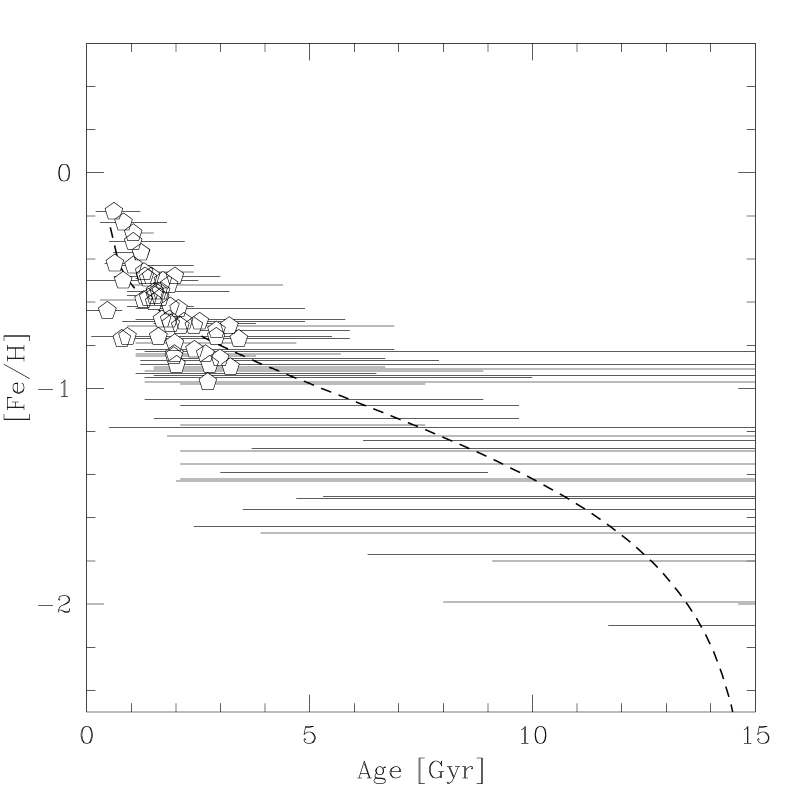
Figure 11: The age-metallicity relation of our sample. Ages derived by comparison with stellar evolution models of Girardi et al. (2000). The horizontal bars are the 95% age confidence intervals for each star. The most likely age is indicated by a pentagon, when the confidence interval is smaller than 5 Gyr. The dotted line illustrates the prediction of a closed-box model with constant star formation rate and a remaining gas fraction of 0.0018 at $t=0.5$ Gyr.

Age estimates were computed for our objects by calibrating the age dependence of the RGB with Padova stellar evolution models (Girardi et al. 2000). Figure 11 shows the resulting age estimates versus the metallicities obtained from the Ca II  triplet. The horizontal bars show the 95% confidence interval of the age determination given the observational uncertainties. The most likely age values and the confidence intervals were computed following the Bayesian approach of Pont & Eyer (in prep.). Bayesian probability theory allows a realistic computation of the probability distribution function of a derived quantity, here the age, when the relative uncertainties are high (see for instance Sivia 1996). In such cases, a simpler approach often leads to systematic biases and underestimated error intervals. The possible presence of AGB stars would slightly increase the computed ages for a fraction of the sample (by $\sim$0-1 Gyr for young objects), the AGB being slightly bluer than the RGB in most cases. Note that reasonable changes in the metallicity calibration do not affect the fundamental features of these results, young ages being imposed to a large fraction of the sample by the fact that the metal-rich Fornax giants are much bluer than globular clusters of similar metallicities.

Fig. 11 gives an indication of the age-metallicity relation of Fornax. The constraint on ages get stronger for stars with ages below 5 Gyr. The emerging picture (ensuring coherence between the spectroscopic and photometric data on Fornax red giants) is that Fornax underwent an initial stage of enrichment reaching [Fe/H]$\sim-1$ about 3 Gyr ago. Then, sustained star formation progressively increased the ISM [Fe/H] to a recent value of at least $\sim-$0.5 dex. The metal enrichment curve of a closed-box model is plotted on Fig. 11 for comparison.

Table 5 shows the result of sorting the ages of the stars into four intervals and provides an indication of their age distribution. To infer information about the star formation rate of Fornax as a whole from this distribution, the statistical corrections calculated in Section 3.2 from synthetic models were applied. As a result, Table 5 would imply a significant increase in the star formation rate in the last $\sim$4 Gyr.

These conclusions are affected by the uncertainties in the relative lifetimes of stars of different ages near the tip of the RGB. In fact, our experience with synthetic CMD studies (Gallart et al. 1999; Gallart, Aparicio & Bertelli 2003) shows that the number counts of stars near the tip of the RGB is difficult to match consistently with the number of stars in other parts of the CMD. Zoccali & Piotto (1999) found good agreement between the observed and theoretical luminosity functions of the main-sequence, subgiant-branch and RGB of old globular clusters in a range of metallicities. A similar study involving clusters of different ages is highly needed.

4.2 Other clues from the CMD

Is our picture compatible with parts of the CMD other than the RGB? The Fornax CMD contains numerous features associated with a particular age and metallicity, namely a weak horizontal branch, a prominent red clump with a long tail at the bright end, and a main sequence extending to $M_{I}\sim-$0.5. These features indicate respectively a weak old metal-poor population, an intermediate-age population of various ages and metallicities, and a very recent population, down to $\simeq$500 Myr old. All of these are qualitatively compatible with the picture obtained from the RGB and the calcium triplet.

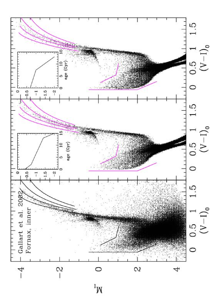
Figure 12: Left: Observed CMD for the central 6.7′$\times$ 6.7′of Fornax, obtained using FORS at the VLT, and published in Gallart et al. (2002). A set of lines bracketing the upper observed main sequence, and the Armandroff and Da Costa (1991) sequences for the globular clusters M15, M2, NGC1851 and 47 Tuc, have been drawn as a reference. Middle: synthetic CMD obtained assuming a constant star formation rate between 12 Gyr and 0.5 Gyr ago, the Kroupa et al. (1993) IMF, 25% binary stars, and the AMR shown in the inset, which is a fit to the AMR displayed in Figure 11. Right: same as middle panel, but modifying the assumed AMR to the one shown in the corresponding inset, which is approximated from the AMR derived by Saviane et al. (2000) from the position of the stars in the RGB (in both synthetic CMDs, a gaussian metallicity dispersion from the mean AMR has been introduced, with $\sigma(z)$=0.0005 at all ages).The position of the stars on the RGB does not match exactly in the observed and synthetic samples, and this is a known major drawback of current stellar evolution models when used to fit CMDs. The position of main-sequence stars predicted by the models, however, is much more reliable, and a good agreement is found between the positions of the main sequence in the observed CMD and the synthetic CMD in the middle panel, computed using the AMR obtained in the current spectroscopic analysis. Both main sequences are nicely centered in the brackets. The main sequence in the right panel, however, is displaced to the blue with respect to the observed main sequence, due to the lower metallicities of the stars younger that 2 Gyr.

To check the compatibility of our AMR with the observed CMD more quantitatively, we produced a synthetic CMD using the AMR obtained above –approximated by a linear interpolation between the values (Gyr, Z)= (15, 0.0002), (13, 0.0008), (2, 0.0036), (0,0.008)– and constant star formation rate between 12 and 0.5 Gyr (see Figure 12, and its caption, for more details). In Figure 12, this synthetic CMD (middle panel) is compared to the Fornax observations (left panel). A visual comparison shows that the main features are well reproduced in the model, except for the fact that the position of the RGB is not perfectly matched, which is a well-known problem of current stellar evolutionary models Since the main sequence is the theoretically best understood feature in a CMD, particularly important is the good agreement between the position and shape of the observed and synthetic upper main-sequence, which are both well centered within the corresponding reference lines. Since the AMR has been obtained from information on the RGB exclusively, this is a completely independent consistency check indicating that the spectroscopically derived metallicities are in good agreement with the observed CMD.

As a comparison, we computed a synthetic CMD with a slightly different AMR (as can be deduced from Saviane et al. 2000) whose main difference with the AMR inferred by us is a lower metallicity for the 1-2 Gyr old population. This CMD is represented in the right panel of Figure 12. Note that the post-main sequence features are quite similar in the two synthetic models, and that the main difference is in the position of the upper main sequence, which is too blue when the lower metallicity AMR is used. This further indicates that the high metallicity, young end of the AMR is a feature not only suggested by the spectroscopic measurements, but necessary to obtain a good match with the young part of the observed CMD.

5 Discussion: Fornax as a Local Group dwarf galaxy

The metallicity distribution and AMR that we derive for Fornax make it a complex system, more reminiscent of the LMC (Pagel & Tautvais̆ienė 1998) or the Milky Way’s disk (Rocha-Pinto et al. 1996, Edvardsson et al. 1993) than of other dwarf spheroidals. Like those two systems and unlike most other dwarf spheroidals, Fornax has a rather metal-rich main population, with a tail of old and metal-poor stars. Also like these two systems, its AMR is compatible with a rapid initial enrichment, followed by a period of slower enrichment, and then a recent acceleration of the enrichment.

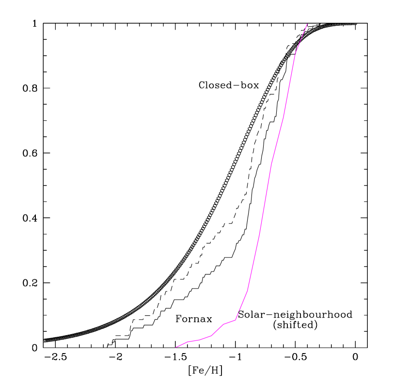
Figure 13: The cumulative metallicity distribution for Fornax – solid line: our sample, broken line: underlying population – compared to a closed-box model and to the data of Jørgensen (2000) for the Galactic disc (shifted by 0.6 dex).

Fig. 13 compares the cumulative metallicity distribution of Fornax with that of a ”closed-box” model and the Galaxy. Although there is also a departure from the closed-box model in Fornax, the distribution is significantly nearer to a closed-box relation than the Galaxy. This is probably even more true when the outer parts of Fornax are taken into account. The inclusion of the outer parts in the cumulative metallicity distribution will proportionally increase the number of very metal-poor objects.

Consequently, there appears to be no need to invoke a large infall of unenriched gas on the galaxy or a large loss of enriched gas. Moreover, the almost complete absence of young, metal-poor stars would seem to exclude a scenario of accretion of relatively pristine gas for late star formation episodes.

5.1 Where is the gas?

The Fornax results strongly reinforce the mystery posed by the complete absence of gas in dwarf spheroidal galaxies (Knapp, Kerr & Bowers 1978). Fornax seems to have been producing large amounts of stars continuously until very recent times. Then, as we observe it, it has stopped forming stars and disposed of every trace of gas. We could be observing Fornax just after its last star formation episode, similar to Carina and Leo I. Dwarf irregulars could be equivalent galaxies forming stars at the present time. However, the situation would still be statistically unlikely. If Fornax has been forming stars up to 200 Myr ago (Saviane et al. 2000), it would be a surprising coincidence to observe it this close to the time when its gas was rapidly enriched and then completely expelled.

A more satisfactory solution would be if some gas is hidden but still at the disposal of Fornax. Blitz & Robishaw (2000) reported several dSph galaxies with HI in the vincinity. While several of these detections were not confirmed (e.g., Young 1999), and some even retracted (Blitz, priv. comm.), the HI around the Sculptor galaxy has been confirmed by Carignan et al. 1998. Fornax was unfortunately not included in the Blitz & Robishaw study because it was outside the area covered by the Dwingaloo survey. Given its history of continuous and recent star formation, we would predict that significant amounts of gas associated with Fornax might still be detected in its vicinity.

Another conclusion of Blitz & Robishaw (2000) is that dSph nearer than 250 pc to a giant galaxy (the Galaxy or M31) contain much less gas, an effect that the authors attribute to ram-pressure stripping. Fornax is well within this distance limits, and we would accordingly expect it to contain little or no gas. We may still, then, be viewing Fornax by accident just after its ”gas death”, during what may be its first passage very near the Milky Way. The precise determination of the proper motion of Fornax and a computation of its likely orbit will provide a test of this scenario (see Piatek et al. 2002 for a preliminary estimate).

5.2 Comparison with evolutionary models of dwarf galaxies.

It is interesting to compare the properties of Fornax with the predictions by Mac Low & Ferrara (1999, MF99) and Ferrara & Tolstoy (2000, FT00). In order to identify where is Fornax in the MF99 parameter space, we will derive its baryonic mass, and an estimate of its likely SNe rate from data in the literature. The total (dark plus baryonic) mass of Fornax is $\sim 7\times 10^{7}$ (Mateo 1998); by assuming the $(M/L)_{tot,V}=4.4$ given in the same paper, and a baryonic $M/L\simeq 1.0$ (calculated for a population with constant star formation rate from 12 to 0.5 Gyr ago), this corresponds to a baryonic mass of $M_{g}=1.6\times 10^{7}M_{\odot}$. For a constant star formation rate, it corresponds to a rate of 1400 $M_{\odot}$ Myr^-1. For a Salpeter IMF, and this star formation rate, 170 $M_{\odot}$ Myr^-1 of stars would be produced in the mass interval of SNe II progenitors, 10-100 $M_{\odot}$, with mean mass $\simeq 20M_{\odot}$. These figures imply a rate of $\simeq$ 8.5 SNe/Myr, or a SNe luminosity $\simeq 2.7\times 10^{38}$ ergs s^-1. If we input these data in Tables 2 and 3 of MF99, we find that the mass ejection efficiency expected for Fornax would be modest, $\simeq 1\times 10^{-2}$, while all the metals should be ejected. The fact that there is a substantial metal enrichment in Fornax seems to be in contradiction with these models, and would indicate that the metal ejection efficiency must be in some way overestimated in them.

Is the model more representative for the smallest dSphs? Making the same calculation as above for a system with baryonic mass $M_{g}=3\times 10^{5}M_{\odot}$, and assuming a constant star formation rate active in them for a maximum of $\simeq 5Gyr$, we get an upper limit for the star formation rate of 60 $M_{\odot}$ Myr^-1, or 0.3 SNe Myr^-1. This is the lower limit of SNe rate considered by Mac Low & Ferrara, who predict that these galaxies are also expected to keep some gas through their lifetimes but to lose all metals produced by type II SNe. This may be compatible with their enrichment being substantially lower than that of Fornax. However, lower star formation rates and therefore lower SNe rates than calculated above must be invoked for some fraction of the galaxy’s lifetime in order to explain the still noticeable enrichment of the gas reflected in the metallicity of their stars (Shetrone, Côté & Sargent 2001 and several earlier studies). Tamura et al. (2001) have proposed a possible solution that may work at the lowest metallicities. They note that star formation may be strongly regulated in low metallicity gas by the lack of coolants (Nishi & Tashiro 2000). But once the metallicity rises to [Fe/H]$\simeq-$2, the metals become effective coolants, and the subsequent star formation should produce SNe that expel their metals as described by MF99 and FT00. This is inconsistent with the observational data for Draco, Sextans, and Ursa Minor (Shetrone et al. 2001), which show that they contains substantial numbers of stars that are more metal-rich than this limit.

One possible reason for the apparent overestimate of metal ejection efficiency in the MF99 and FT00 models is the fact that they consider that all the mass injection occurs in the central 100 pc of the galaxy. As MF99 discuss, several small bubbles distributed in a larger area must be less effective in blowing away the ISM than a single central cluster. The core radius of Fornax is 460 pc and that of the smaller galaxies is $\simeq 200$ pc. Since dwarf irregular galaxies show spatially and chronologically segregated sites of star formation (as beautifully shown by Dohm-Palmer et al. 2002), it is possible that the assumption of one large central site for the dSph galaxies is also incorrect.

Further hints may be provided by high resolution spectra abundances of individual elements. Shetrone et al. (2001, 2003) note that all the dSph have an under-abundance of even-Z elements compared with the Milky Way halo, which may indicate a large contribution by type Ia SNe, either because SNe II are less abundant in these galaxies or because their ejecta are not retained. Could it be that the ejecta from type Ia SNe are retained more than that of type II, and that this provide some extra enrichment? One property of SNe Ia which is different from SNe II is that they are expected to be isolated events, i.e. less spatially clustered and likely to be less synchronized in time than SNe II. According to FT00, isolated SNe events would not cause blowout and would have a lower metal ejection efficiency. There seems to be one difference between the Fornax abundance patterns and that of other dSph, according to Shetrone et al. (2003): while there is a general trend of decreasing [$\alpha$/Fe] abundance with increasing metallicity in the observed dSph, in Fornax the even-Z ratios appear flat to slightly rising, even if still under-abundant. All this seems to indicate that the enrichment mechanisms are similar in dSph regardless of their mass. The slightly different tendency of even-Z ratios with metallicity in Fornax may simply reflect the more extended period of star formation in this galaxy compared to the other dSph. This discussion, however, is based on very few stars. High resolution spectra of a large number of stars will provide very important information to understand the enrichment mechanisms in dSph galaxies, and the processes driving their evolution.

6 Summary and conclusions

We obtained spectroscopy in the Ca II  triplet region of the spectrum for 117 stars in the Fornax dSph galaxy using FORS1 at the VLT. We derived metallicities for them using our own $\Sigma$Ca-M_I-[Fe/H] calibrations, based on observations of Ca II  line strengths in 11 globular clusters plus M67, M11 and the LMC. We show evidence that a calibration against M_I instead of the most commonly used one in terms of V-V(HB) may produce more accurate results for the young populations present in Fornax. Our main conclusion is that there is a tail of very metal-rich RGB stars in Fornax, with metallicities ranging from approximately $-$0.7 to $-$0.4, whose existence could not have been suspected from their color in the CMD. The metallicities of these stars, combined with their relatively blue colors, imply that they have ages of the order of 2 Gyr.

We use synthetic CMDs to examine how the age and metallicity distribution of our sample is related to that of the whole population. Combining the metallicity data with constraints from the position of the same stars in the CMD, we find that the Ca II data are compatible with only a narrow range of possible AMR, which in turn, allow to put some constraints on the SFH. It appears that Fornax underwent very substantial chemical enrichment in the last few Gyr, from [Fe/H]$\sim-1.0$ up to [Fe/H]$\sim-0.4$. Its AMR is nearer to a Closed-Box model than that of the Galaxy. The large number of young ($<4$ Gyr old) stars that we infer from the combination of their metallicity and their position on the CMD would imply a star formation rate somewhat rising (by a factor of $\sim$2) in the last 2-4 Gyr. However, this last result depends on an extrapolation from the RGB population to the total population that is not very reliable with the present models.

This scenario corresponds remarkably well with observed features in the CMD other than the RGB, and in particular, with a robust feature (in terms of our stellar evolution knowledge) as is the main sequence. Indeed, the derived AMR, and in particular, the high metallicity tail, produces synthetic CMDs with upper main-sequence colors totally compatible with the observed one, whereas a lower metallicity for the youngest stars would produce too blue a main sequence.

Appendix A Theoretical sensitivity of the Ca II triplet to age and metallicity.

Under the usual assumption that abundance, effective temperature (T_e) and surface gravity (log g) are the main parameters determining the strengths of absorption lines, the combined equivalent width of the Ca II  triplet ($\Sigma$Ca), evolves along a surface in the (T_e, log g, [Ca/H], $\Sigma$Ca) space. Consequently, to relate abundances to the measurable parameter, $\Sigma$Ca, the parameters T_e and log g must be fixed in some way. It was found empirically (Da Costa 1998; Armandroff & Da Costa 1991; Olszewski et al. 1991) that for globular clusters a plot of $\Sigma$Ca against absolute V or I magnitude or against the closely related quantity V-V(HB), the difference in V magnitude between a red giant and the mean V of the horizontal branch, produces an accurate ranking of globular clusters by metallicity. The precision in [Fe/H] that one can obtain for individual red giants using $\Sigma$Ca and, for example, V-V(HB) is quite high ($\leq\pm 0.2$ dex), and this technique has developed into the most popular way of using low resolution spectra to estimate the abundances of stars in globular clusters and dSph galaxies. Before applying this method to the red giants in Fornax, we need to understand why it works well for globular cluster stars and its limitations for a mixture of ages and compositions.

The globular clusters in the Milky Way are very old, and for the purposes of our discussion their age differences can be ignored. With the exception of a very few clusters, most notably $\omega$ Cen, the stars within a globular cluster have very nearly the same chemical composition. These facts explain why in the CMD, the RGBs of globular clusters are tight sequences of stars that are offset from one another in order of the metallicities of the clusters, as predicted by stellar evolutionary theory for clusters of uniform age but varying composition. Since T_e, log g, and luminosity vary monotonically along the RGB, one can use measures of T_e, typically B-V or V-I, or measures of luminosity, M_V, M_I, or V-V(HB), which is independent of both reddening and distance, as indicators of position on the RGB. It is known empirically that plots of $\Sigma$Ca against any one of these luminosity indicators provides better metallicity discrimination than a plot against an indicator of T_e. To understand why this is so let us consider the sensitivity of $\Sigma$Ca to T_e and log g using the calculations that Jorgensen, Carlsson, & Johnson (1992) made of $\Sigma$Ca for stars in the ranges $4000<$T_e$<6600$, $4.0<\log g<0.0$, and $-1.0<[A/H]\leq+0.2$, under the assumption of NLTE. For estimates of T_e  and $\log g$ for the red giants, we will use the Padova isochrones (Girardi et al. 2000). It is important to note that the calculations by Jorgensen et al. (1992) and by Girardi et al. (2000) assumed solar mixes of elements. While there is clear observational evidence that [Ca/Fe] is not solar in at least some Fornax stars (Shetrone et al. 2003), their departures are small in comparison to the effects that we describe below, which provide only a qualitative description of the behavior of the Ca II lines. To avoid confusion with predictions for specific abundance ratios, we will use [A/H] to indicate overall metallicity when discussing the CaII line strengths.

Figure 14 shows the most luminous portions of the RGB in the log T_e- log g plane for four different metallicities (Z=0.001, 0.004, 0.008, and 0.019, which assuming Z$\sun$ = 0.02 corresponds to [Fe/H]= $-$1.30, $-$0.70, $-$0.40, and $-$0.02, respectively). The quantities are plotted so that this diagram resembles an H-R diagram, in that T_e increases to the left and luminosity increases toward the top. Representative lines of constant I and V absolute magnitude are shown. As in the H-R diagram, the RGB’s of different Z form a nearly parallel sequence of curves. At every $\log~{}g$, the most metal-rich RGB has the coolest T_e. A vertical line in Figure 14 indicates that there is a T_e below which the CaII lines are seriously blended with a TiO band. The location of this line was estimated from the V-I colors of red giants having significant TiO absorption in the very old, metal-rich open cluster NGC 6791 (Garnavich et al. 1994) and the more metal-poor globular cluster 47 Tuc (Lloyd Evans 1974). While this line is approximate, it illustrates the observed fact that $\Sigma$Cacannot be measured to the RGB tip in 47 Tuc ($[Fe/H]=-0.7$) and in more metal-rich globular clusters.

According to the calculations of Jorgensen et al. (1992), at fixed T_e and log g, $\Sigma$Ca increases with increasing [A/H]. At fixed [A/H] and log g and over the T_e range of the RGB’s in Figure 14, $\Sigma$Ca increases with increasing T_e, with the exception that for [A/H]=$-$1, it decreases slightly for log g $\geq 2$. At fixed [A/H] and T_e, these calculations show that for log g $\leq 2$, $\Sigma$Ca increases with decreasing log g. This is much more pronounced at [A/H]=0.0 than at lower abundances, and in fact for [A/H]=$-$1 $\Sigma$Ca has little gravity sensitivity except between log g = 1 and 0. Figure 14 illustrates that going along a line of constant absolute I or V magnitude from the Z=0.001 RGB to the one for Z=0.019, both log T_e and log g decrease. The decrease in T_e tends to weaken $\Sigma$Ca, while the decrease in log g tends to strengthen it. The two effects roughly cancel. The dependence of $\Sigma$Ca on [A/H] ensures that RGB’s of different Z will be separated in a plot of $\Sigma$Ca against absolute I or V magnitude or V-V(HB), as is observed.

A similar argument explains why $\Sigma$Ca changes by only a small amount along the RGB of a globular cluster. As luminosity increases, the accompanying decreases in T_e and $\log~{}g$ weaken and strengthen $\Sigma$Ca, respectively, which results in only a modest increase in $\Sigma$Ca with luminosity ($\delta$$\Sigma$Ca$/\delta M_{I}\sim~{}0.5$). This explains why in the absolute magnitude vs. $\Sigma$Ca diagram, the RGB’s of globular clusters are well approximated by straight lines. It is remarkable, however, that these lines have the same slope to within the errors over a wide range in metallicity. In the log T_e- $\log g$ plane, the RGB’s of different Z are almost straight lines and approximately parallel (see Fig. 14). If the partial derivatives of $\Sigma$Ca with respect to log T_e and $\log~{}g$ are nearly constant for all metallicities, then the RGB’s will be lines of similar slope in the absolute magnitude vs. $\Sigma$Ca diagram. This is not the case according to the calculations of Jorgensen et al. (1992), which predict that Ca II strength increases more rapidly with decreasing log $g$ at high metallicity than at low, which should cause an increase in the slope with increasing metallicity in the absolute magnitude vs. $\Sigma$Ca diagram (see Fig. 16). It is surprising that this effect is not clearly evident in the data (see Section 3.1).

We have also illustrated in Figure 14 the curve for a constant color of V$-$I=1.4, which as expected is nearly a line of constant T_e. This curve illustrates why plotting $\Sigma$Ca against V$-$I or another color sensitive to T_e produces relatively poor separations between the RGB’s of different metallicities. Along a line of constant V$-$I, T_e remains essentially constant, but log g increases substantially from the metal-poor to the metal-rich RGB. These differences in gravity weaken the dependence of $\Sigma$Ca on metallicity and tend to push together the RGB’s of globular clusters in plots of W(Ca II) against color. This effect and the sensitivity of color to errors in the reddening corrections make plots of $\Sigma$Ca against color much less useful than plots against absolute magnitude.

In this article we calibrate $\Sigma$Ca against metallicity for a mixed-age population. It is very instructive to make similar comparisons of RGB’s holding Z fixed, but varying the ages of the populations. We have plotted in Figure 15 the Padova isochrones for 12.6 and 0.25 Gyrs and Z=0.019. A line of constant absolute I magnitude is also plotted, and along this line we have marked the locations of the isochrones for this composition and ages of 12.6, 4.0, 1.0, 0.5, and 0.25 Gyrs. For ages $\leq 1$ Gyr, the RGB terminates near $M_{I}\approx-3$, and the more luminous stars of these ages are AGB stars. Since the AGB and RGB are almost coincident in the log T_e- log g plane (see Fig. 15), the ambiguity about whether a star belongs to the AGB or the RGB has only a small effect on the interpretation of its $\Sigma$Ca. Figure 15 illustrates the important point that at a constant absolute magnitude, the isochrones for younger ages have higher T_e and larger $\log g$ than do ones for older ages. Because $\Sigma$Ca is affected in opposite ways by these differences, age differences have only small effects on plots of $\Sigma$Ca against $M_{I}$ or $M_{V}$. The differences in T_e  and log g between the 12.6 and 4.0 isochrones are so small that their effects on $\Sigma$Ca nearly perfectly cancel. This is not the case for differences between the 12.6 isochrone and the ones for ages $\leq 1$ Gyr, but nonetheless the M_I-$\Sigma$Ca remains a very useful diagnostic of metallicity even if there is a large range in age in a stellar population.

Fig. 16 illustrates the weak sensitivity of the M_I-$\Sigma$Ca to age differences. We have used the approximation formulae that Jørgensen et al. (1992, eqs. 7, 9, & 11) derived from fits to their calculations of the sum of the equivalent widths of the two strongest Ca II  lines (8542 and 8662Å) and the Padova isochrones to compute $\Sigma$Ca for stellar populations of different ages and compositions. The values of T_e and log g that are required as input to the Jorgensen et al. (1992) relations for compositions [A/H]=0.0, $-$0.5, and $-$1.0, were obtained from the Padova isochrones for Z=0.019, 0.008, and 0.004, respectively. The last two compositions are not exact matches, but repeating the calculations using instead Z=0.004 and 0.001 for [A/H]=$-$0.5 and $-$1.0, respectively, showed that this has a negligible effect on the $\Sigma$Ca vs. M_I diagram. It has only a small systematic effect on the $\Sigma$Ca vs. V-I diagram in Figure 16 in the sense that the lines of constant composition are separated slightly more in $\Sigma$Ca than they would be if the correct composition was used.

In this article, we have calibrated the $M_{I}$-$\Sigma$Ca diagram using the observed values of $M_{I}$ and $\Sigma$Ca for stars in globular clusters, which have very old ages that are within a few Gyrs of 12.6. We have also used observations of the open cluster M67, which has an age of 4.0 Gyrs and a solar composition (Tautvais̆ienė et al. 2000, and references therein) and the LMC, which has a wide range of ages. According to RGB’s plotted in Fig. 16 for ages of 12.6 and 4.0 Gyrs, very little error in metallicity is introduced by ignoring the age difference between globular clusters and younger systems of the same metallicity.

From previous investigations of the CMD of Fornax, we know that it contains stars that span the age range from the ages of globular clusters down to roughly 0.5 Gyrs (see Introduction). Figure 16 illustrates that over this age range, the M_I-$\Sigma$Ca diagram is mostly sensitive to metallicity and only mildly to age. If, for example, one uses the curves in Figure 16 for 12.6 Gyrs as fiducial curves and then derives values of [A/H] for the stars lying along the curves for 0.25 Gyrs, without taking into account their younger ages, one will underestimate the true abundances of the stars by about 0.2 dex. We have tested this prediction using observations of the open star cluster M11. Note that only a small fraction of the Fornax stars are likely to be this young and that this systematic error decreases substantially with increasing age.

The curves in Figure 16 show that the V-I vs. $\Sigma$Ca diagram is sensitive to age differences, particularly at the highest abundances where $\Sigma$Ca  is more sensitive to surface gravity. While this diagram is less useful for estimating metallicity than the M_I-$\Sigma$Ca diagram, it does provide important information when used in conjunction with this other diagram. Note that on the basis of the M_I-$\Sigma$Ca diagram alone, one could interpret stars lying on the 0.25 Gyr and [A/H]=0.0 curve at, for example M_I=$-$3, as old stars (age $\geq 4$ Gyrs) with $[A/H]\approx-0.2$. Such stars are expected to lie below the curve for [A/H]=0.0 and 4.0 Gyrs in the V-I vs $\Sigma$Ca diagram. If instead they lie above this curve, the first interpretation is incorrect, and the stars are probably younger than 4.0 Gyrs with abundances closer to solar.

Figure 1: Position of the 117 targets on the plane of the sky. Smaller symbols denote targets fainter than I=17.5. The different symbols indicate: hexagons: metal-poor stars ([Fe/H]$<-$1.3); squares: intermediate metallicities; triangles: metal-rich stars ([Fe/H]$>-$0.7). The star symbol indicates the position of the globular cluster located near the center of Fornax.

Figure 3: Sky subtraction procedure for object 103. Top: raw spectrum. The sky emission lines are prominent. The three Ca II  lines are hardly noticeable between them. Middle: the sky spectrum, taken on the side of the object spectrum. Bottom: the final object spectrum, reduced with the offset method. Note the efficiency of the sky subtraction with this method.

Figure 4: Three representative spectra. Top: object with average metallicity ([Fe/H]$\sim-$1). Middle: object with low metallicity ([Fe/H]$\sim-$2). Bottom: spectrum that is too noisy to satisfy our selection criteria. (Note that the average quality of our spectra is significantly higher than in previous studies of Fornax such as Tolstoy et al. 2001).

Figure 5: The positions of the red giants in Fornax (open circles) and in M11 (crosses), compared with the sequences of some clusters, in the (V-I)–M_I color-magnitude diagram (top left), in the $\Sigma$Ca vs. $M_{I}$ plane (top right), in the $\Sigma Ca$ vs. $M_{V}$ plane (bottom left) and in the $\Sigma Ca$ vs. $(V-I)_{0}$ plane (bottom right). The lengths of the lines indicate the range covered by the red giants in the clusters. These clusters were used to calibrate our measurements of the Ca II  triplet as a function of metallicity (see Fig. 7).

Figure 6: Metallicity as a function of $I$ magnitude for our sample. There is no significant increase of the computed metallicity with brightness, implying that the curvature of the calibration towards the brightest magnitudes is limited.

Figure 7: Growth of the Ca II  triplet reduced equivalent width with metallicity. The points indicate the calibrating clusters. The solid line is the cluster calibration (Equ. 1). The dotted line shows the modified relation for young populations with $M_{I}>-3$ (Equation 2), based on the LMC constraint represented by the star symbol. Error bars are from CG (vertical) and from the propagation of the uncertainty on the fits of $\Sigma$Ca vs. $M_{I}$ (horizontal). Note that this figure is a 2-D projection of an actual relation in 4-D space (colour, magnitude, metallicity, Calcium equivalent width). The lines in the figure are projections of the same calibration for different magnitude ranges: $M_{I}\sim-2$ for the clusters and $M_{I}\sim-$4 for the LMC.

Figure 8: LMC (dots) and Fornax (open circles) Ca II triplet data in the $M_{V}$ vs. $\Sigma$Ca plane. The line indicates the slope of isometallicities in the RHS calibration. LMC: Cole et al. (2000). Fornax: this paper.

Figure 9: Histogram: Metallicity distribution of the Fornax red giant sample, based on the $M_{I}$ calibration. The shaded part indicates the less secure part of the calibration, as explained in the text. Dotted line: Inferred metallicity distribution for the underlying population, obtained by applying the corrections suggested by synthetic population modeling (Table 3). The resulting histogram was smoothed with a Normal kernel of $\sigma_{[Fe/H]}=0.1$ dex.

Figure 10: Position of the RGB at a fixed I magnitude in the age-color plane according to the Yonsei-Yale isochrones. The red limit of the Fornax giant branch is indicated as a dashed line.

Figure 14: Position of the red giant branch at t=12.6 Gyr for different metallicities in the log Te vs. log g plane, with some lines of constant color and constant magnitude indicated. The long-dashed line delimits the zone where TiO bands stars affecting the Ca II  triplet region of the spectrum.

Figure 15: Red giant branch and asymptotic giant branch models in the log Te vs. log g for z=0.019. The whole red giant branch locus is indicated for t=12.6 Gyr, and the position of the point at $M_{I}=-3$ mag for different ages.

Figure 16: Ca II  line strength models for red giants in the $M_{I}$ vs. EW (left), $M_{V}$ vs EW (center) and V-I vs EW (right) planes. For the 0.25 Gyr models, both the AGB (dashed curve) and the RGB (solid curve) are plotted. For other ages, only the RGB is plotted. (Note that the relations plotted cannot be used directly to analyse observational data – see footnote 9)

Table 1: Relevant data for the objects measured in the calibration globular clusters. The star designations follow the scheme that Rutledge et al. (1997b) used in their catalog of Ca II measurements, and the photometry is from the same source.

Star ID	V	(B-V)	$v_{obs}$	EW	$\sigma$	EW	$\sigma$	EW	$\sigma$	$\sum(Ca)$	$\sigma$	$\sum(Ca)$	$\sigma$	ID	$\sum Ca$	$\sigma{\sum}$	[Fe/H]CG	$\sigma$[Fe/H]	note
			${\rm kms}^{-1}$	$\lambda_{8498}$		$\lambda_{8592}$		$\lambda_{8662}$		this work		Ru97
NGC 2298
A14	14.35	1.22	147.20	0.79	0.09	2.20	0.11	1.77	0.11	3.66	0.13	3.46	0.13
A17	14.87	1.09	114.60	0.76	0.12	1.94	0.13	1.55	0.13	3.26	0.17	3.20	0.12
A18	14.96	1.00	135.05	0.72	0.14	1.86	0.15	1.54	0.16	3.14	0.20	3.04	0.13
A22	15.30	1.02	127.75	0.64	0.15	1.74	0.17	1.41	0.17	2.91	0.21
A15	14.86	1.12	122.30	0.80	0.11	1.89	0.12	1.50	0.12	3.19	0.15	3.08	0.11
NGC 3201
L2207	14.30	1.07	523.38	0.87	0.13	2.30	0.14	1.88	0.15	3.87	0.18	4.00	0.13
L2214	13.84	1.03	516.21	0.88	0.10	2.17	0.11	1.73	0.12	3.65	0.14	3.67	0.11
L3204	12.29	1.44	479.98	1.26	0.05	3.01	0.05	2.35	0.05	5.05	0.06	5.08	0.03
L3101	13.66	1.16	479.01	1.08	0.10	2.67	0.11	2.06	0.10	4.44	0.13	4.29	0.07
L3102	14.31	1.00	471.67	0.99	0.13	2.25	0.14	1.78	0.15	3.81	0.18	3.80	0.11
L3107	13.38	1.14	474.90	0.96	0.09	2.44	0.09	1.88	0.09	4.05	0.12	4.11	0.07
L4215	13.56	1.26	514.17	0.95	0.09	2.51	0.10	1.99	0.10	4.17	0.12	4.32	0.12
L4307	14.33	1.11	502.04	0.93	0.12	2.33	0.13	1.87	0.14	3.92	0.17	3.82	0.11
L4318	12.54	1.45	493.45	1.17	0.05	2.97	0.05	2.35	0.05	4.97	0.06	5.03	0.03
L1309	13.26	1.03	487.97	0.94	0.08	2.48	0.08	1.91	0.09	4.09	0.11	4.16	0.08
NGC 7099
DP24	13.06	1.09	-271.84	0.72	0.17	1.95	0.19	1.53	0.19	3.23	0.24	3.20	0.10
DP23	12.20	1.40	-170.28	0.86	0.10	2.29	0.11	1.84	0.11	3.82	0.13	3.64	0.10
DP91	13.00	1.06	-122.12	0.79	0.18	1.81	0.18	1.45	0.18	3.07	0.23	3.04	0.10
D31	14.22	0.81	-118.27	0.54	0.20	1.47	0.22	1.12	0.22	2.41	0.27
D57	14.93	0.73	-140.11	0.63	0.31	1.45	0.32	1.15	0.34	2.46	0.41	2.21	0.19
DP19	13.14	1.04	-128.02	0.79	0.11	1.77	0.11	1.41	0.12	3.01	0.14	2.91	0.04

Table 2: Fornax star data. Photometry from Gallart et al. (in prep.). [Fe/H]_CG is the metallicities on the Carretta & Gratton (1997) scale. Key to the notes: see bottom of the Table.

ID	alpha	delta	V	$\sigma$V	R	$\sigma$R	I	$\sigma$I	V-I	$\sum Ca$	$\sigma{\sum}$	[Fe/H]CG	$\sigma$[Fe/H]	note
101	2 40 08.42	$-$34 25 33.89	18.607	0.005	17.755	0.004	17.037	0.010	1.570	7.29	0.24	$-$0.3 :	0.10
102	2 40 06.56	$-$34 25 22.57	19.032	0.007	18.306	0.005	17.700	0.015	1.332	6.22	0.33	$-$0.6 :	0.14	3
103	2 40 05.07	$-$34 24 38.39	18.646	0.006	17.917	0.004	17.299	0.016	1.347	4.85	0.22	$-$1.38	0.09
104	2 40 02.76	$-$34 23 32.92	18.527	0.006	17.645	0.004	16.868	0.020	1.659	6.28	0.18	$-$0.8 :	0.08
105	2 40 01.13	$-$34 25 09.72	18.208	0.005	17.434	0.003	16.752	0.020	1.456	4.78	0.16	$-$1.54	0.07
106	2 39 57.97	$-$34 23 20.69	18.425	0.005	17.642	0.003	16.948	0.027	1.477	5.32	0.29	$-$1.22	0.12	g
107	2 39 57.06	$-$34 23 32.81	–	–	–	–	(18.287)	–	–	6.47	0.42	–	–	7
108	2 39 54.32	$-$34 23 31.10	18.371	0.004	17.547	0.003	16.900	0.020	1.471	5.00	0.26	$-$1.40	0.11
109	2 39 53.17	$-$34 22 58.75	–	–	–	–	(17.261)	–	–	3.86	0.25	$-$1.82	0.11	1,g
110	2 39 51.33	$-$34 24 53.41	18.683	0.005	17.876	0.005	17.235	0.023	1.448	5.73	0.29	$-$0.97	0.12	3
111	2 39 49.78	$-$34 23 52.76	18.559	0.008	17.846	0.006	17.256	0.021	1.303	4.76	0.21	$-$1.43	0.09
112	2 39 48.58	$-$34 24 48.48	19.033	0.009	18.263	0.006	17.883	0.009	1.150	5.81	0.26	$-$0.8 :	0.11
113	2 39 46.05	$-$34 25 04.52	19.040	0.009	18.286	0.004	17.663	0.017	1.377	7.14	0.26	$-$0.3 :	0.11
114	2 39 43.92	$-$34 23 59.85	18.595	0.005	17.895	0.004	17.268	0.017	1.327	3.78	0.22	$-$1.85	0.09
115	2 39 43.55	$-$34 26 12.39	19.441	0.010	18.733	0.006	18.122	0.014	1.319	6.04	0.39	–	–	7
116	2 39 40.84	$-$34 24 29.66	18.768	0.006	17.990	0.005	17.313	0.012	1.455	5.02	0.22	$-$1.28	0.09
117	2 39 38.42	$-$34 23 47.92	18.466	0.004	17.798	0.004	17.187	0.011	1.279	4.45	0.22	$-$1.59	0.09
202	2 40 22.11	$-$34 27 11.00	18.674	0.005	17.933	0.004	17.307	0.011	1.367	6.63	0.22	$-$0.5 :	0.09
203	2 40 18.15	$-$34 27 56.60	18.808	0.007	18.072	0.005	17.461	0.011	1.347	6.73	0.23	$-$0.4 :	0.10	4
204	2 40 17.88	$-$34 27 01.20	18.513	0.024	17.654	0.030	16.918	0.020	1.595	6.24	0.17	$-$0.8 :	0.07
205	2 40 15.97	$-$34 27 04.30	18.726	0.009	17.935	0.007	17.270	0.009	1.456	5.71	0.20	$-$0.97	0.08
206	2 40 15.04	$-$34 26 39.40	18.942	0.007	18.163	0.005	17.509	0.008	1.433	6.75	0.23	$-$0.4 :	0.10
207	2 40 13.44	$-$34 26 19.20	18.524	0.005	17.647	0.003	16.919	0.006	1.605	7.01	0.17	$-$0.4 :	0.07
208	2 40 12.89	$-$34 25 38.10	18.978	0.009	18.267	0.006	17.675	0.007	1.303	5.71	0.25	$-$0.9 :	0.11
209	2 40 12.30	$-$34 25 19.20	18.515	0.006	17.653	0.003	16.938	0.006	1.577	6.20	0.17	$-$0.8 :	0.07
210	2 40 10.39	$-$34 25 18.20	18.411	0.006	17.565	0.004	16.870	0.007	1.541	5.69	0.16	$-$1.07	0.07
211	2 40 06.50	$-$34 26 12.70	18.784	0.006	18.016	0.005	17.366	0.010	1.418	6.44	0.22	$-$0.6 :	0.09
212	2 40 05.62	$-$34 25 36.30	18.637	0.006	17.928	0.004	17.316	0.012	1.321	4.54	0.19	$-$1.53	0.08
213	2 40 05.52	$-$34 24 26.90	18.935	0.007	18.222	0.004	17.617	0.014	1.318	6.26	0.25	$-$0.6 :	0.11
214	2 40 03.93	$-$34 24 12.60	18.503	0.007	17.661	0.004	16.930	0.017	1.573	7.02	0.19	$-$0.4 :	0.08	1
215	2 40 00.22	$-$34 24 53.90	19.205	0.010	18.496	0.006	17.754	0.015	1.451	6.26	0.29	$-$0.6 :	0.12	2
216	2 39 56.58	$-$34 26 06.60	19.092	0.007	18.364	0.006	17.730	0.025	1.362	–	–	–	–	7
217	2 39 56.25	$-$34 25 04.80	–	–	–	–	(17.487)	–	–	5.61	0.29	$-$0.9 :	0.12
218	2 39 56.04	$-$34 24 11.60	–	–	–	–	(17.067)	–	–	6.59	0.20	$-$0.6 :	0.08
301	2 39 31.43	$-$34 22 00.40	18.755	0.005	–	–	17.471	0.005	1.284	3.60	0.27	$-$1.88	0.11
302	2 39 31.86	$-$34 22 25.00	18.364	0.005	–	–	16.828	0.004	1.536	4.78	0.20	$-$1.52	0.08
303	2 39 33.33	$-$34 22 43.20	18.920	0.006	–	–	17.504	0.007	1.416	5.87	0.26	$-$0.8 :	0.11
304	2 39 31.43	$-$34 23 05.30	18.664	0.006	17.836	0.005	17.125	0.007	1.539	6.15	0.22	$-$0.8 :	0.09
305	2 39 23.44	$-$34 23 10.40	19.231	0.007	18.489	0.006	17.838	0.010	1.393	–	–	–	–	7
306	2 39 19.00	$-$34 23 41.70	18.785	0.006	18.007	0.004	17.320	0.020	1.465	5.55	0.22	$-$0.98	0.09
307	2 39 28.80	$-$34 24 13.00	18.551	0.006	17.702	0.004	16.974	0.007	1.577	5.88	0.19	$-$0.96	0.08
308	2 39 33.55	$-$34 24 41.80	18.499	0.006	17.581	0.003	16.766	0.005	1.733	6.68	0.19	$-$0.6 :	0.08
309	2 39 27.88	$-$34 24 49.40	18.686	0.005	17.975	0.004	17.338	0.007	1.348	4.19	0.22	$-$1.68	0.09
310	2 39 30.28	$-$34 25 15.70	18.688	0.005	18.026	0.004	17.417	0.007	1.271	2.97	0.23	$-$2.07	0.10
311	2 39 33.56	$-$34 25 49.50	18.569	0.006	17.706	0.003	16.965	0.004	1.604	6.70	0.21	$-$0.6 :	0.09
312	2 39 35.40	$-$34 26 05.90	19.118	0.006	18.417	0.005	17.774	0.008	1.344	5.00	0.30	$-$1.17	0.13
313	2 39 32.40	$-$34 26 35.40	19.051	0.007	18.461	0.006	17.919	0.010	1.132	5.87	0.33	$-$0.7 :	0.14
314	2 39 33.06	$-$34 26 50.40	18.950	0.007	18.183	0.005	17.511	0.009	1.439	5.70	0.23	$-$0.9 :	0.10
315	2 39 26.05	$-$34 27 06.80	19.157	0.008	18.434	0.005	17.805	0.015	1.352	5.62	0.30	$-$0.92	0.13
316	2 39 27.40	$-$34 27 27.70	19.213	0.007	18.460	0.004	17.840	0.013	1.373	6.65	0.32	$-$0.4 :	0.13
317	2 39 21.75	$-$34 27 46.70	18.837	0.009	18.056	0.004	17.387	0.014	1.450	5.76	0.24	$-$0.9 :	0.10	4
318	2 39 19.35	$-$34 28 11.80	18.936	0.007	18.238	0.005	17.646	0.015	1.290	4.17	0.29	$-$1.62	0.12
402	2 40 06.48	$-$34 28 53.50	18.407	0.004	17.542	0.004	16.827	0.006	1.580	5.89	0.18	$-$0.98	0.08
403	2 40 03.74	$-$34 29 35.57	18.934	0.007	18.256	0.005	17.661	0.009	1.273	4.16	0.25	$-$1.62	0.11	5
405	2 39 59.67	$-$34 28 46.20	18.781	0.005	18.064	0.005	17.423	0.011	1.358	5.78	0.24	$-$0.9 :	0.10
406	2 39 59.85	$-$34 28 12.80	18.774	0.006	18.052	0.006	17.423	0.016	1.351	5.76	0.24	$-$0.91	0.10
407	2 39 58.73	$-$34 27 49.50	18.553	0.009	17.870	0.004	17.257	0.016	1.296	6.08	0.23	$-$0.8 :	0.10
408	2 39 54.77	$-$34 28 35.40	18.809	0.006	18.131	0.005	17.560	0.012	1.249	5.95	0.24	$-$0.8 :	0.10
409	2 39 52.80	$-$34 28 36.80	18.882	0.007	18.054	0.004	17.386	0.013	1.496	6.66	0.23	$-$0.5 :	0.10
410	2 39 50.67	$-$34 29 07.00	19.211	0.008	18.508	0.005	17.901	0.012	1.310	5.62	0.29	$-$0.9 :	0.12
411	2 39 50.29	$-$34 28 14.20	18.695	0.006	17.991	0.004	17.404	0.013	1.291	3.95	0.22	$-$1.76	0.09
412	2 39 48.66	$-$34 28 07.50	19.100	0.010	18.381	0.005	17.764	0.012	1.336	5.37	0.26	$-$1.02	0.11
413	2 39 46.38	$-$34 28 20.70	18.605	0.006	17.807	0.004	17.106	0.012	1.499	5.42	0.18	$-$1.12	0.08
414	2 39 45.30	$-$34 27 38.20	18.669	0.008	17.846	0.004	17.138	0.012	1.531	6.23	0.20	$-$0.8 :	0.08
415	2 39 42.29	$-$34 28 28.30	18.119	0.006	17.423	0.004	16.787	0.007	1.332	5.41	0.17	$-$1.21	0.07
416	2 39 46.62	$-$34 28 10.00	18.538	0.007	17.685	0.004	16.939	0.006	1.599	6.09	0.18	$-$0.9 :	0.08
417	2 39 38.40	$-$34 28 31.90	19.507	0.010	18.820	0.007	18.218	0.011	1.289	6.01	0.37	$-$0.6 :	0.16
418	2 39 36.31	$-$34 28 22.70	18.539	0.005	17.549	0.003	16.604	0.006	1.935	4.05	0.17	$-$1.87	0.07	1
502	2 40 28.64	$-$34 28 25.70	18.688	0.006	17.928	0.005	17.250	0.013	1.438	5.65	–	$-$1.00	0.08	g
503	2 40 32.32	$-$34 30 54.30	18.657	0.006	17.862	0.005	17.172	0.009	1.485	6.47	–	$-$0.6 :	0.10	g
504	2 40 27.65	$-$34 29 30.30	19.118	0.009	18.366	0.006	17.722	0.012	1.396	6.76	–	$-$0.4 :	0.10	g
505	2 40 26.45	$-$34 30 18.20	18.796	0.008	17.992	0.005	17.292	0.011	1.504	6.57	–	$-$0.6 :	0.10	g
506	2 40 22.37	$-$34 29 26.90	18.435	0.006	17.794	0.004	17.231	0.012	1.204	4.22	–	$-$1.69	0.06	g
507	2 40 22.74	$-$34 30 27.60	18.446	0.005	17.610	0.004	16.920	0.011	1.526	5.48	–	$-$1.13	0.08	g
508	2 40 22.08	$-$34 30 43.90	19.003	0.007	18.253	0.005	17.624	0.013	1.379	6.02	–	$-$0.7 :	0.09	g
509	2 40 16.72	$-$34 29 35.60	18.428	0.005	17.529	0.003	16.789	0.007	1.639	5.88	–	$-$1.00	0.08	g
510	2 40 15.90	$-$34 29 47.20	18.764	0.007	17.981	0.005	17.328	0.008	1.436	6.40	–	$-$0.6 :	0.09	g
511	2 40 16.73	$-$34 30 55.70	19.117	0.009	18.385	0.005	17.771	0.010	1.346	6.65	–	$-$0.4 :	0.12	g
512	2 40 13.90	$-$34 30 36.60	18.545	0.006	17.644	0.004	16.890	0.004	1.655	6.79	–	$-$0.5 :	0.09	g
513	2 40 14.84	$-$34 32 08.20	18.701	0.008	17.939	0.005	17.282	0.007	1.419	4.86	–	$-$1.37	0.08	g
514	2 40 13.41	$-$34 32 15.40	18.913	0.044	17.925	0.862	17.740	0.149	1.173	6.23	–	$-$0.6 :	0.10	g
515	2 40 10.15	$-$34 31 49.30	19.119	0.009	18.393	0.006	17.756	0.009	1.363	5.93	–	$-$0.8 :	0.10	g
516	2 40 06.53	$-$34 31 01.00	18.430	0.005	17.596	0.006	16.886	0.006	1.544	5.18	–	$-$1.28	0.07	g
517	2 40 05.96	$-$34 32 01.40	18.567	0.007	17.768	0.004	17.083	0.006	1.484	5.04	–	$-$1.31	0.07	g
518	2 40 05.48	$-$34 32 43.20	18.521	0.007	17.634	0.003	16.899	0.005	1.622	6.39	–	$-$0.7 :	0.09	g
519	2 40 03.40	$-$34 32 12.60	18.847	0.008	18.052	0.005	17.368	0.006	1.479	6.27	–	$-$0.7 :	0.09	g
702	2 39 45.12	$-$34 29 36.50	18.736	0.006	18.016	0.005	17.339	0.006	1.397	6.14	0.27	$-$0.8 :	0.11
703	2 39 37.97	$-$34 29 34.80	18.934	0.007	18.156	0.005	17.462	0.009	1.472	5.43	0.24	$-$1.06	0.10
704	2 39 34.59	$-$34 29 49.40	18.632	0.005	17.781	0.003	17.053	0.007	1.579	5.90	0.17	$-$0.93	0.07
705	2 39 33.75	$-$34 30 12.20	19.125	0.008	18.433	0.005	17.792	0.013	1.333	5.13	0.26	$-$1.12	0.11
706	2 39 32.46	$-$34 30 34.30	–	–	–	–	(18.730)	–	–	6.46	0.42	$-$0.3	0.18	4,6
707	2 39 28.33	$-$34 30 38.90	18.999	0.013	18.243	0.073	17.643	0.203	1.356	5.57	0.26	$-$0.95	0.11
708	2 39 32.22	$-$34 31 07.10	18.750	0.007	17.972	0.004	17.268	0.007	1.482	5.83	0.21	$-$0.91	0.09
709	2 39 28.64	$-$34 31 29.50	18.553	0.006	17.763	0.005	17.069	0.006	1.484	5.63	0.19	$-$1.00	0.08
710	2 39 32.95	$-$34 32 09.10	18.570	0.005	17.808	0.004	17.134	0.005	1.436	6.71	0.20	$-$0.5 :	0.08
711	2 39 37.17	$-$34 32 40.10	18.768	0.006	17.995	0.005	17.309	0.006	1.459	5.64	0.22	$-$0.99	0.09
712	2 39 26.18	$-$34 32 28.00	–	–	–	–	(17.295)	–	–	7.08	0.24	$-$0.3 :	0.10
713	2 39 34.09	$-$34 33 12.20	18.703	0.006	17.853	0.004	17.128	0.006	1.575	6.65	0.20	$-$0.6 :	0.08
714	2 39 34.10	$-$34 33 35.70	18.486	0.005	17.650	0.003	16.934	0.004	1.552	5.83	0.18	$-$0.99	0.08
715	2 39 33.39	$-$34 34 01.20	18.598	0.005	17.796	0.004	17.094	0.006	1.504	5.94	0.18	$-$0.9 :	0.08
716	2 39 28.07	$-$34 34 03.90	18.598	0.005	17.796	0.004	17.094	0.006	1.504	5.71	0.20	$-$1.01	0.08
717	2 39 27.83	$-$34 34 23.10	18.903	0.007	18.136	0.006	17.454	0.006	1.449	6.26	0.24	$-$0.7 :	0.10
718	2 39 24.84	$-$34 34 40.80	18.618	0.005	17.787	0.004	17.050	0.005	1.568	6.71	0.21	$-$0.5 :	0.09
802	2 40 18.99	$-$34 34 07.10	19.012	0.006	18.293	0.005	17.678	0.008	1.334	5.30	0.28	$-$1.07	0.10
803	2 40 21.45	$-$34 35 21.80	18.796	0.006	18.021	0.004	17.356	0.009	1.440	6.07	0.24	$-$0.8 :	0.10
804	2 40 16.73	$-$34 34 34.30	18.757	0.006	17.950	0.004	17.270	0.005	1.487	6.65	0.22	$-$0.5 :	0.09
805	2 40 19.25	$-$34 36 12.50	18.634	0.007	17.795	0.003	17.096	0.007	1.538	6.18	0.21	$-$0.8 :	0.09
806	2 40 18.86	$-$34 36 42.80	18.707	0.007	17.912	0.003	17.244	0.010	1.463	6.42	0.23	$-$0.6 :	0.10
807	2 40 17.18	$-$34 36 57.60	18.787	0.006	18.072	0.004	17.467	0.008	1.320	5.75	0.26	–	–	7
809	2 40 16.72	$-$34 34 54.80	18.248	0.004	17.479	0.003	16.830	0.005	1.418	3.49	0.18	$-$2.01	0.08
810	2 40 09.39	$-$34 36 18.10	18.402	0.005	17.593	0.004	16.939	0.005	1.463	5.91	0.18	$-$0.95	0.08
811	2 40 05.09	$-$34 35 42.90	18.660	0.006	17.968	0.004	17.368	0.006	1.292	3.17	0.21	$-$2.03	0.09
812	2 40 04.99	$-$34 36 34.00	18.484	0.005	17.648	0.003	16.954	0.005	1.530	5.41	0.19	$-$1.18	0.08
813	2 40 07.99	$-$34 38 11.80	18.393	0.005	17.617	0.004	16.961	0.006	1.432	5.16	0.20	$-$1.30	0.08
814	2 40 05.05	$-$34 37 47.50	18.366	0.005	17.536	0.003	16.856	0.006	1.510	5.75	0.17	$-$1.04	0.07
815	2 40 00.21	$-$34 36 55.90	19.465	0.009	18.843	0.007	18.222	0.011	1.243	3.85	0.35	–	–	7
816	2 40 00.72	$-$34 38 05.40	18.720	0.006	17.940	0.004	17.281	0.008	1.439	6.48	0.24	$-$0.6 :	0.10
817	2 39 58.91	$-$34 37 55.00	18.944	0.006	18.249	0.005	17.634	0.009	1.310	5.79	0.27	$-$0.8 :	0.11

Table 3: Expected metallicity bias in our sample.

Metallicity	Ratio
range	selected vs. total
$-2.0$ – $-1.8$	0.80
$-1.8$ – $-1.6$	0.70
$-1.6$ – $-1.4$	0.73
$-1.4$ – $-1.2$	0.70
$-1.2$ – $-1.0$	0.91
$-1.0$ – $-0.8$	1.00
$-0.8$ – $-0.6$	1.48
$>-0.6$	1.15

Table 4: Expected age bias in our sample.

Age	Ratio	Proportion
range	selected vs. total	of AGB
1-3	1.35	43%
3-5	1.35	16%
5-7	0.96	17%
7-9	0.93	21%
9-11	0.78	25%
11-13	0.73	15%
13-15	0.90	24%

Table 5: Inferred age distribution and star formation rate.

Age	Stars	Corrected	Corresponding
interval	in sample	to total	SFR
		population	(mean=1)
0-2 Gyr	35	26	2.4
2-4 Gyr	31	23	2.1
$>4$ Gyr	27	34	0.6

References

- (1) Alcaino, G. & Liller, W. 1986, A&A, 161, 61
- (2) Alcaino G., Liller W., & Alvarado F. 1989, A& A 216, 68
- (3) Armandroff T.E., & Da Costa G.S. 1991, AJ 101, 1329
- (4) Armandroff, T. E., &Zinn R. 1988 AJ 96, 92
- (5) Aparicio, A., Carrera, R., & Martínez-Delgado, D. 2001, AJ, 122, 2524
- (6) Bertelli G., Bressan A., Chiosi C., Fagotto F., & Nasi E., 1994, A&AS 106, 275
- (7) Blitz, L., & Robishaw, T. 2000, ApJ 541, 675
- (8) Buonanno, R., Corsi, C. E., Zinn, R., Fusi Pecci, F., Hardy, E., & Suntzeff, N. B. 1998, ApJ 501, 33
- (9) Buonanno, R., Corsi, C. E., Castellani, M., Marconi, G., Fusi Pecci, F., & Zinn, R. 1999, AJ, 118, 1671
- (10) Caldwell, N., Armandroff, T.E., Da Costa, G. S., & Seitzer, P. 1998, AJ, 115, 535
- (11) Carney, B. W. 1996, PASP, 108, 900
- (12) Carrera, R., Aparicio, A., Martinez-Delgado, D., & Alonso-Garcia, J. 2002, AJ 123, 3199
- (13) Carretta, E., Cohen, J.G., Gratton, R.G., & Behr B.B. 2001, AJ 122, 1469
- (14) Carretta, E., Gratton, R. G. 1997, A&AS 121, 95 [CG]
- (15) Cenarro, A. J., Gorgas, J., Cardiel, N., Pedraz, S., Vazdekis, A., & Peletier, R. F. 2001a, Ap&SS Suppl. 277,319
- (16) Cenarro, A. J., Cardiel, N., Gorgas, J., Peletier, R. F., Vazdekis, A., Prada, F. 2001, MNRAS 326, 959
- (17) Cole, A.A., Smecker-Hane, T.A., & Gallagher, J.S. 2000, AJ 120, 1808
- (18) DaCosta] Da Costa G.S. 1988, in The Harlow-Shapley Symposium on Globular Cluster Systems in Galaxies, Proceedings of the 126th IAU Symposium, p. 217, Ed. J.E. Grindlay & A.G. Davis Philip
- (19) Da Costa, G.S., & Armandroff, T.E. 1990, AJ, 100, 162
- (20) Da Costa, G.S., & Armandroff, T.E. 1995, AJ 109, 2533
- (21) Da Costa, G.S., & Hatzidimitriou, D. 1998, AJ 115, 1934
- (22) Da Costa, G.S., Hatzidimitriou, D., Irwin, M.J., & McMahon, R.G. 1991, MNRAS, 249, 473
- (23) Demarque, P., Zinn, R., Lee, Y.-W., & Yi, S. 2000, AJ 119, 1398
- (24) Demers, S., Irwin, M.J., & Kunkel, W.E. 1994, AJ 108, 1648
- (25) Dickens, R.J. 1972, MNRAS, 157, 299
- (26) Dohm-Palmer, R. C., Skillman, E. D., Mateo, M., et al. 2002, AJ 123,813
- (27) Edvardsson, B., Andersen, J., Gustafsson, B. et al. 1993, A&AS 102, 603
- (28) Ferrara, A., & Tolstoy, E. 2000, MNRAS, 313, 291
- (29) Gallart, C., Aparicio, A., & Bertelli, G. 2003, Coimbra Experiment: Group I Analysis, in “ Observed HR diagrams and stellar evolution models: the interplay between observational constraints and theoretical limitations”, Eds. T. Lejeune & J. Fernandes. ASP Conference Series, in press.
- (30) Gallart, C., Freedman, W.L., Aparicio, A., Bertelli, G., & Chiosi, C. 1999, AJ 118, 2245
- (31) Gallart, C., Zinn, R., Pont, F., Hardy, Ed., Marconi, G., & Buonanno, R. 2002, The Messenger, No. 108, p. 16
- (32) Garnavich, P.M., VandenBerg, D.A., Zurek, D.R., and Hesser, J. E. 1994, A.J., 107, 1097
- (33) Girardi, L., Bressan, A., Bertelli, G., & Chiosi, C. 2000, A&AS 141, 371
- (34) Gonzalez, G., & Wallerstein, G. 1998, AJ, 116, 765
- (35) Gonzalez, G., & Wallerstein, G. 2000, PASP, 112, 1081
- (36) Harris W.E. 1996, AJ 112, 1487 (VizieR Catalog VII/195) L91
- (37) Hurley–Keller, D., Mateo, M., & Grebel, E.K. 1999, ApJ, 523, L25
- (38) Hurley–Keller, D., Mateo, M., & Nemec, J. 1998, AJ, 115, 1840
- (39) Janes, K.A., & Smith G.H. 1984, A.J. 89, 487
- (40) Jørgensen, U.G., Carlsson, M., & Johnson H. R., 1992, A&A 254, 258
- (41) Jørgensen, B.R. 2000, A&A 363, 947
- (42) Knapp, G. R., Kerr, F.J., & Bowers, P.F. 1978, ApJ 83, 360
- (43) Kroupa, P., Tout, C.A., & Gilmore, G. 1993, MNRAS 262, 545
- (44) Layden A.C., Sarajedini A. 2000, AJ 119, 1760
- (45) Lee, S.-W. 1977, A&AS, 28, 409
- (46) Lehnert, M.H., Bell, R.A., Hesser, J.E., & Oke, J.B. 1992, ApJ, 395, 466
- (47) Lloyd Evans, T. 1974, MNRAS, 167, 393.
- (48) Luck, R.E., Moffett, T.J., Barnes, T.G., & Gieren, W. 1998, AJ 115, 605
- (49) Mac Low, M.-M., & Ferrara, A. 1999, ApJ, 513, 142
- (50) Mateo, M. 1998, ARA&A 36, 435
- (51) Mateo, M., Olszewski, E., Welch, D. L., Fischer, P., & Kunkel, W. 1991, AJ, 102, 914
- (52) Mighell, K.J., & Burke, C.J. 1999, AJ, 118, 366
- (53) Mighell, K.J., & Rich, R.M. 1996, AJ, 111, 777
- (54) Nishi, R., & Tashiro, M. 2000, ApJ, 537, 59
- (55) Olszewski, E.W., Schammer, R.A., Suntzeff, N.B., & Harris, H.C. 1991, AJ 101, 515
- (56) Ortolani, S., Bica, E., & Barbuy, B. 1992, A& AS 92, 441
- (57) Ortolani, S., Barbuy, B., & Bica, E. 1990, A& A 236, 362
- (58) Pagel B.E.J., Tautvaisiene G. 1998. MNRAS 299, 535
- (59) Piatek, S., Pryor, C., Olszewski, E. W., Harris, H. C., et al. 2002, AJ 124, 3198
- (60) Richer, H. B., Fahlman, G. G., Rosvick, J., Ibata, R. 1998, ApJ 504, L91
- (61) Rocha-Pinto H.J., Maciel W.J.1996, MNRAS 279, 447
- (62) Rutledge, G. A., Hesser, J. E., & Stetson, P. B. 1997a, PASP 109, 883 [RHS]
- (63) Rutledge G. A., Hesser J. E., Stetson, P. B. et al. 1997b, PASP 109, 907
- (64) Saviane, I., & Rosenberg, A. 1999, The Galactic Halo: From Globular Cluster to Field Stars, Proceedings of the 35th Liege International Astrophysics Colloquium, Edited by A. Noels et al. (Liege, Belgium), 197
- (65) Saviane, J., Held, E.V., & Bertelli, G. 2000, A&A 355, 56
- (66) Schlegel, D.J., Finkbeiner, D.P., Davis M. 1998, ApJ 500, 525
- (67) Shetrone, M.D., Bolte, M., & Stetson, P.B. 1998, AJ, 115, 1888
- (68) Shetrone, M.D., Côté, P., & Sargent, W.L.W. 2001, ApJ, 548, 592
- (69) Shetrone, M.D., & Keane, M.J. 2000, AJ 119, 840
- (70) Shetrone, M.D., Venn, K.A., Tolstoy, E., Primas, F., Hill, V., & Kaufer, A. 2003, AJ, 125, 684
- (71) Sivia D. S. 1996, Data analysis – a Bayesian tutorial, Oxford University Press
- (72) Smecker-Hane, T. A., Stetson, P. B., Hesser, J. E., & van den Bergh, D. A. 1996, in From stars to galaxies: the impact of stellar physics on Galaxy evolution (ed. C. Leitherer, U. Fritze-van Alvensleben & J. Huchra), ASP Conf Series, vol. 98, 328
- (73) Smecker-Hane, T.A., Mandushev, G.I., Hesser, J.E., Stetson, P.B., Da Costa, G.S., & Hatzidimitriou, D. 1999, in Spectrophotometric dating of stars and Galaxies, ASP Conference Proceedings, Ed.: I. Hubeny, S. Heap, and R. Cornett., Vol. 192, 159
- (74) Sneden, C., Kraft, R. P., Shetrone, M.D., Smith, G. H., Langer, G. E., & Prosser, C. F. 1997, AJ 114, 1964.
- (75) Stetson, P.B., Hesser, J., & Smecker-Hane, T.A. 1998, PASP, 110, 533
- (76) Sung, H., Bessell, M.S., Lee, H.-W., Kang, Y. H., & Lee, S.-W. 1999, MNRAS 310, 982
- (77) Suntzeff, N.B., Aaronson, M., Olszewski, E.W, & Cook, K.H. 1986, AJ, 91, 1091
- (78) Suntzeff, N.B., Mateo, M., Terndrup, D.M., Olszewski, E.W., Geisler, D., & Weller, W. 1993, ApJ, 418, 208
- (79) Suntzeff, N.B., Schommer, R.A., Olszewski, E.W., & Walker, A.R. 1992, AJ 104, 1742
- (80) Tamura, N., Hirashita, H., & Takeuchi, T.T. 2001, ApJ, 552, L113
- (81) Tautvais̆ienė, G., Edvardsson, B., Tuominen, I., & Ilyin, I. 2000, A&A 360, 499
- (82) Tolstoy, E., Irwin, M. J., Cole, A.A., Pasquini, L., Gilmozzi, R., & Gallagher, J. S. 2001, MNRAS, 327, 918
- (83) Tolstoy, E., Venn, K.A., Shetrone, M., Primas, F., Hill, V., Kaufer, A., & Szeifert, T. 2003, AJ, 125, 707
- (84) Twarog, B.A., Ashman, K.M., & Anthony-Twarog, B.J. 1997, AJ 114, 2556
- yi (2001) Yi, S., Demarque, P., Kim, Y.-C., Lee, Y.-W., Ree, C.H., Lejeune, Th., & Barnes, S. 2001, ApJS, 136, 417
- (86) Young, L.M. 1999, AJ, 117, 1758
- (87) Young, L.M. 1999, AJ, 119, 188
- (88) Zinn, R. 1981, ApJ, 251, 52
- (89) Zinn R., & Barnes S. 1996, AJ 112, 1054
- (90) Zoccali, M., & Piotto, G. 2002, A&A, 358, 934