Microlensing Candidates in M87 and the Virgo Cluster
with the Hubble
Space Telescope
The position of the giant elliptical galaxy M87 at the center of the Virgo Cluster means that the inferred column density of dark matter associated with both the cluster halo and the galaxy halo is quite large. This system is thus an important laboratory for studying massive dark objects in elliptical galaxies and galaxy clusters by gravitational microlensing, strongly complementing the studies of spiral galaxy halos performed in the Local Group. We have performed a microlensing survey of M87 with the WFPC2 instrument on the Hubble Space Telescope. Over a period of thirty days, with images taken once daily, we discover seven variable sources. Four are variable stars of some sort, two are consistent with classical novae, and one exhibits an excellent microlensing lightcurve, though with a very blue color implying the somewhat disfavored possibility of a horizontal branch source being lensed. Based on sensitivity calculations from artificial stars and from artificial lightcurves, we estimate the expected microlensing rate. We find that the detection of one event is consistent with a dark halo with a 20% contribution of microlensing objects for both M87 and the Virgo Cluster, similar to the value found from observations in the Local Group. Further work is required to test the hypothesized microlensing component to the cluster.
1 Introduction
In a classic paper Paczyński (1986) proposed a search for massive dark objects in the Milky Way halo by searching for the rare gravitational microlensing of Large and Small Magellanic Cloud (LMC and SMC) stars. For a halo consisting of roughly solar–mass objects, of order one in one million LMC stars is being lensed (with a magnification of 30% or more) at any given time. An extensive monitoring campaign could thus hope to detect these transient lensing events, which develop over typically 100 days, thus elucidating the nature of the Milky Way halo. This has been accomplished with great success by several groups, described below. Furthermore, the extension of this work to other nearby galaxies is well underway.
The MACHO project (Alcock et al. 2000) monitored the LMC for microlensing events for the better part of a decade: they conclude that there is an excess of events over the expectation from known stellar populations corresponding to an approximately 20% contribution of sub-solar-mass objects to the dark halo of the Milky Way. The EROS collaboration (Afonso et al. 2003) has monitored the LMC and SMC over a similar time period, and finds only an upper limit of 25% on the microlensing component.
As proposed a decade ago (Crotts 1992), the Andromeda Galaxy (M31) is an excellent target for a microlensing survey. Both the Milky Way and M31 halos can be studied in detail. Very few stars are resolved from the ground, thus image subtraction is required. This is the “pixel” lensing regime (Crotts 1992; Baillon et al. 1993; Gould 1996). Several collaborations, including MEGA (preceded by the VATT/Columbia survey), AGAPE, and WeCAPP, have produced a number of microlensing event candidates involving stars in M31 (Crotts & Tomaney 1996, Ansari et al. 1999, Aurière et al. 2001, Uglesich 2001, Calchi Novati et al. 2002, de Jong et al. 2003, Riffeser et al. 2003). The results of the VATT/Columbia survey (Uglesich et al. 2003) are inconclusive, possibly indicating the presence of a microlensing halo of sub-solar-mass objects around M31.
Finally, we turn to the subject of this paper, the giant elliptical galaxy M87 in the Virgo cluster. The ability of the Hubble Space Telescope (HST) to perform a microlensing survey of the Virgo cluster was noted several years ago (Gould 1995). A variability survey of M87 could discover a microlensing population either in the M87 halo or even an intracluster population in the overall Virgo halo. We have used thirty orbits of HST data from the WFPC2 to perform just such a survey.
All of these observational programs are aimed at understanding the nature of the dark halos of galaxies. The halos of the large spiral galaxies of the local group (the Milky Way and M31) can be studied from the ground. M87 is a particularly interesting target because it is an elliptical galaxy, and as such contains a different population of stars. Furthermore, it serves to “illuminate” any dark objects in the halo of the Virgo cluster. Such objects might have been stripped from their host galaxies in the formation of Virgo, as the tidal effects during galaxy mergers and other interactions should have been substantial.
The outline of this paper is as follows. We briefly discuss the theory of microlensing in §2. Our HST observations of M87, data reduction, and image subtraction and filtering are covered in §3. Selection of candidate events, including the exclusion of hot pixels is discussed in §4. We describe the variable source detection efficiency in §5, and the calculation of the microlensing rate in §6. We conclude with a discussion in §7.
2 Theory of Microlensing
The term microlensing refers to the fact that the multiple images of source stars are split by microarcseconds. The splitting is unobserved, but the magnification can be large. It is the transient magnification that is sought.
2.1 Basics
We now lay out the basic physics and terminology of gravitational microlensing. For a point mass, the lens equation can be written in terms of the Einstein radius and angle, given by
| (1) |
where is the lens mass, is the distance to the lens, is the distance to the source, and is the distance between the lens and source. In angular coordinates, the lens equation relating source position and image position is then
| (2) |
There are always two images. This equation is usually written with all angles written in units of the Einstein angle. In particular . The magnification was first given by Einstein (1936):
| (3) |
For , , namely the magnification can be very large.
The timescale over which a microlensing event progresses is the Einstein time , given in terms of the Einstein radius and the perpendicular velocity of the lens relative to the line of sight to the source . Assuming rectilinear motion for the lens, we find
| (4) |
where is the minimum impact parameter of the lens. For a star with unlensed flux , the microlensing lightcurve is then
| (5) |
If can be measured, the Einstein time can be extracted from the event lightcurve. The shape of the lightcurve does contain some information on (and thus ), though extracting it requires very high quality data (e.g. Paulin-Henriksson et al. 2003).
This discussion has assumed that the angular size of the source is much smaller than the minimum impact parameter in Einstein units, namely . If this is not the case, finite source size effects can be significant, as summarized by Yoo et al. (2004).
2.2 “Pixel” Microlensing
Unfortunately, the unlensed flux of the source star is not easy to measure. Even nearby sources (e.g. in the LMC) may be significantly blended. For sources in M87, the blending is always severe, and the unlensed flux is all but unmeasurable. The Einstein timescale is notoriously hard to determine for such events. The measured timescale is in effect the full width at half maximum timescale, given by , where
| (6) |
with limiting behavior
| (7) |
For all values of we thus find that . For the present work, high magnifications are required, implying small values of , and thus full width at half maximum timescales much smaller than the Einstein timescales.
In the high magnification limit , we can write down the “degenerate” form of the microlensing lightcurve,
| (8) | |||||
| (9) |
where is the baseline flux and is a fit parameter expressing the maximum increase in flux from the lensed star. In the absence of blending , but for M87 in practice blending is significant. This is the “pixel” lensing regime in which sources are only resolved when they are lensed. The measured parameters are and . As mentioned previously, the Einstein time can not be easily measured without measuring , though for high signal-to-noise data (Paulin-Henriksson et al. 2003) this problem is ameliorated. We can proceed however, though a distribution in for microlensing events is not as useful as a distribution in . In the high magnification regime, we note that (though this relation is affected by finite source size effects), so we can recover Einstein times statistically at least, given that the distribution of is known (Gondolo 1999). This distribution is simply the stellar luminosity function. Stellar population models can give a reasonable estimate for the luminosity function, and the first non-trivial moment is known: this is just the surface brightness fluctuation (SBF) magnitude.
3 Observations and Image Analysis
3.1 Design of the Observational Program
Our HST microlensing program, GO-8592, was awarded 30 orbits for WFPC2 imagery in May/June 2001; a journal of observations is presented in Table 1. This allocation comprised a program of daily single-orbit sampling of M87 over a month-long interval. Within each orbit we obtained four 260s exposures in the -band F814W filter, yielding a 1040s total exposure, followed by a single 400s broad-R F606W exposure to obtain color information for any variables identified. The four F814W pictures were dithered by steps of 0.5 WFC-pixels aligned with the CCD axes, which in the -band allows a Nyquist-sampled interlace image to be constructed for the WFC CCDs (Lauer 1999a); the PC1 CCD is already critically-sampled at F814W. In passing, the sharper PSF at F606W would require a dither pattern to lift the aliasing. This schema establishes the F814W frames as the primary search imagery, relegating the F606W to providing auxiliary color information and verification of the events. To obtain equal quality in F606W (or another bluer filter) would be prohibitive; microlensed stars are expected to be red, requiring more than a double allocation of orbits. The alternative of splitting a single orbit equally between two filters would reduce the depth in any single filter, and would make dithering prohibitively expensive. While the dithering scheme that we did adopt does include an overhead that might otherwise be used to collect photons, this exposure-time penalty is more than offset by the resolution gain returned by Nyquist sampling. A simpler strategy of obtaining single, or CR-split identical exposures, in each filter within an orbit would reduce the sensitivity to detecting faint point-sources against the M87 envelope. The nucleus of M87 was centered in PC1. The pointing and orientation were held fixed over the full interval of the search. The orientation showed no significant variations over the program, while the pointing repeated to better than a single WFC pixel; as we discuss below, this was actually less optimal than using a few PSFs-worth of pointing dither between the daily visits.
3.2 Basic Image Preparation
The initial image reduction goal was to generate a Nyquist-sampled F814W super-image for each WFC CCD from the dither sequence for each daily visit. This task included repair of charge traps, hot pixels, and cosmic ray events prior to the actual reconstruction of the super image. Fortunately, the dithers were executed with sufficient accuracy that this later step could be simply done by interlacing the four images within the dither sequence. Each original image contributed one pixel to each a pixel box in the super-image; the scale of the super-image is twice as fine as that of the source images. Lauer (1999a) presents an algorithm for constructing this image had the dithers not been exact 0.5 pixel steps, but in practice this method was not required.
Since the images in each dither set had slightly different pointings, the standard method of removing cosmic ray events (CRE) by comparing two exposures with identical positioning and integration times could potentially misidentify point sources moving with respect to the CCD pixels as cosmic ray events. For the WFC images in the present data set, an initial interlace image was constructed, and the intensity of each pixel was compared to the average of its neighbors. Pixels that were discrepant at the level (where was estimated from a WFPC2 noise-model, rather than from the deviation about the average), and that had a value in excess of that of the average (to avoid flagging the peaks of point sources centered on one pixel in the sequence), were flagged as CRE. Pixels neighboring any given hit in the individual exposures were considered to be part of the same event if they deviated from the interlaced image neighboring pixel average by After the initial round of CRE identification, pixels affected by the hits were deleted from the average neighboring pixel frame, and additional events were identified in two more rounds of CRE identification. After all CRE were identified, affected pixels were replaced by the average of the remaining unaffected neighbors in the interlace frame. In practice this procedure appeared to work extremely well for removing CRE.
In the case of the PC1 data, as the dither steps were only slightly larger than the PC pixel scale, detection and repair of CRE were easier. The images in a given dither set were simply compared under the assumption that the offsets were a single pixel in amplitude. The average pixel values used to replace the CRE in this regard should be better estimates than those used in the WFC dither sets. After the CRE were repaired, the individual PC1 images in the dither set were shifted to a precise common origin by sinc-function interpolation (e.g. Castleman 1995) and combined.
During an initial reduction of the complete dataset, the brighter hot pixels were often identified as CRE. True hot pixels were identified as deviant pixels that appeared at a constant CCD location over the duration of the observations. Unfortunately, a large population of low-level hot pixels escaped initial detection; an additional population of hot pixels consisted of those that newly arose within the month-long duration of the program. Most of these could be identified by visual inspection of the interlaced super-images. Residual hot pixels in the interlaced image for any given day made a readily-identifiable artifact consisting of a block of elevated sub-pixels. When one day’s interlaced image was blinked against those surrounding it in time, the small day-to-day pointing variations additionally helped to isolate hot pixels from compact astronomical sources. The program had actually specified pointing varying by from day to day, thus the small pointing differences were fortuitous for identifying hot pixels. The pointing errors were typically less than . Random variations in the lowest-level hot pixels, however, made them difficult to distinguish from true point-sources with this small amount of pointing jitter; residual hot-pixels are the most important source of false positive detections of variable sources. A more optimal program design would include a somewhat larger pointing dither between repeat visits to allow for complete decoherence between source and detector structure.
3.3 Preparation of the Images for Variable Source Detection
Detection of variables in M87 is discussed in detail in the next section, but briefly variables are identified by examining the temporal run of residual intensity values at any pixel location after the WFC interlaced images and PC1 stacked images have been registered to a common origin, have had the average intensity value subtracted, and were processed with an optimal filter.
As noted above the pointing varied slightly from day to day. Fortunately, the rich M87 globular cluster system provided ample astrometric references. Centroids of a few dozen clusters in each CCD field allowed precise angular offsets to be derived for each day’s images (presented in Table 1). The roll angle was held fixed over this interval to better than 0.05 degrees. The images were then shifted to a common origin by sinc-function interpolation; which does not degrade the resolution of Nyquist-sampled images. The full dataset (excluding the images for day-12, which had excessive jitter) could then be stacked to make a precise average image of M87, which in turn was subtracted from each day’s data. While in principle this step might be omitted, in practice it greatly eases the examination of each day’s images by removing the strong intensity of the background galaxy, fixed point sources, and the fine structure associated with the envelope SBF pattern (essentially the Poisson noise associated with the numbers of bright stars falling in resolution elements).
Processing each day’s residual image with an optimal filter provides for the best detection of a point source against a noisy background. The relationship between the filtered image, and the initial difference image, is given as:
| (10) |
where is a model of the expected backgrounds (e.g. surface brightness + read noise) at any pixel location, is the PSF, and is its transpose, and indicates convolution (Castleman 1995). The filtering effectively performs an optimally-weighted integration of any point sources present in the difference image. The normalization converts the intensity scale to significance in units of the locally-weighted dispersion, . The filtered image is essentially the detection significance for a point source centered at . A point source will appear in for several around the true location, but the local maximum of indicates the best fit position of the source. As for the CRE detection above, the noise-image was based on the averaged image of M87 and the WFPC2 detector properties. PSFs were calculated using the TINY-TIM package; for the subsampled WFC images, the Lauer (1999b) pixel response function was applied to the TINY-TIM PSFs to provide the best fidelity on the diffraction scale.
4 Selection of Candidate Events
The optimally filtered images described in the previous section are now analyzed as a time series for the extraction of variable sources. The analysis proceeds in several steps. First, a baseline is calculated at each pixel. Next, pixels that exhibit consecutive significant deviations from the baseline are recorded and grouped, and centroids are estimated. These are the level-1 candidates. Each level-1 candidate lightcurve is classified according to a number of template fits. Furthermore the level-1 candidates are compared to a hot pixel list. The resulting candidates are the level-2 candidates. These are visually inspected, eliminating obvious subtraction artifacts that are not hot pixels. The remaining candidates are considered real astrophysical sources.
4.1 Baseline Selection
The first stage in the search for variable sources is the selection of the baseline level. A source that flares will have several bright points, which are included in the reference image. Thus, the baseline flux will be lower than that in the reference image. We have studied several criteria for setting the baseline, and settled on one, as we now describe.
The most naive baseline selection is obviously that the reference image is the baseline. This is unsatisfactory since for a given peak flux, the baseline would depend on the timescale.
A better choice for the baseline would be to take a subset of the individual fluxes and call the average the baseline. For example, taking the average of the ten lowest points on the lightcurve as the baseline works reasonably well. As only one third of the data is involved, even slowly varying sources should be detected. However, this baseline selection is also unsatisfactory, as it is quite vulnerable to downward fluctuations in flux: in fact it selects for them.
We improve the “lowest ten” baseline selection of the previous paragraph by requiring that the ten points be consecutive. We allow wraparound for candidates that flare in the middle of the time series, e.g. the average of the first four and the last six points can be the baseline. This selection is less vulnerable to downward fluctuations due to the consecutivity. As such, we use this definition of the baseline level in all of the following analysis. Varying the number of samples taken doesn’t have much effect, though taking too many eliminates slowly varying sources and taking too few makes the baseline quite noisy. Essentially, we are constructing a running reference image of ten individual images, and taking the lowest such image for each pixel individually as the baseline.
4.2 Variability Selection
Having set the baseline using the running reference image as in §4.1, we now search for sources that vary about the baseline significantly. We study two minimum thresholds of and relative to a baseline only fit, or equivalently a signal-to-noise ratio of about 7 and 10, respectively. The required signal-to-noise ratio can be accumulated over several images, and we use several different tests.
We first apply a basic consecutivity test, namely several consecutive images exhibiting a certain significance of detection so that the total gives the threshold . By requiring only a single point, we find that there is too much sensitivity to hot pixels, artifacts, cosmic rays and the like. Requiring two consecutive detections of gives the same total significance and rejects many false detections while allowing fast events to be detected. This is our basic criterion for variability.
We modify this consecutivity test to allow longer timescale events that might be dimmer, though with similar total significance. We test for five consecutive detections, and find more candidates. Extending this test to eight consecutive samples does not yield any new candidates.
These consecutivity tests are sensitive to downward fluctuations ending the consecutive streak. As a check, we use one final test in which the images are averaged in consecutive groups of three, yielding three series of images (1-3, 4-6 etc., 2-4, 5-7, etc., and 3-5, 6-8, etc.) In terms of signal-to-noise ratio, the new image is . The two consecutive test is then applied to these averaged image series.
We have experimented with other similar criteria, e.g. four consecutive, and also requiring a peak sample at higher significance, e.g. five consecutive , including at least one . No new candidates are found in the tests we performed.
We denote sources identified by one or more of the consecutivity tests as the level-1 candidates. There is a high level of duplication here, as we have not grouped candidate pixels together at this stage. This can be done simply by sorting pixels by their and coordinates. An approximate centroid is also calculated at this stage.
4.3 Lightcurve Fitting
Once the level-1 candidates are identified, they are classified according to several template lightcurves. We use four basic templates. First is the trivial constant baseline. The free parameter is simply the baseline level, and the best fit is the average of the points. A two-level baseline (step function) is good for flagging hot pixels. The free parameters are the two baseline levels and the time of the step. We use a linear ramp, though very few level-1 candidates have this as the best fit. There are two free parameters, the slope and intercept. Lastly, we fit the degenerate microlensing lightcurve (which takes the peak magnification to infinity holding the peak flux constant). The parameters are the baseline, the peak time, the peak flux, and the full-width at half maximum timescale.
Each level-1 candidate is fitted to each template, with being calculated. Most level-1 candidates have either the two-level baseline or the microlensing template as the best fit. We discard candidates whose best fit is not the microlensing template, and furthermore we discard events where .
4.4 Hot Pixels
The WFPC2 has a sizable number of hot pixels, which may be confused with astrophysical variable sources. Bright hot pixels are removed along with cosmic ray events (described in §3.2). It is the dimmer hot pixels that are troublesome. Many of these are active at a very low level, and not much concern for imaging, though of crucial concern for a variability search. We attempt to compare sources in the difference images with the PSF to separate the hot pixels from real sources.
We use the difference images directly to identify hot pixels. As many of them are not very active, we average the difference images in consecutive groups of five to improve the sensitivity. If a hot pixel is discovered in any of these stacks, it is flagged so that candidate events at its position can be discarded.
We use a PSF test to identify hot pixels. In the dithered images, a hot pixel should appear as a box. A star (PSF) is more extended than this. We calculate the ratio of the average pixel values in the central four pixels to the average pixel values in the surrounding twelve pixels. In principle this is infinite for a hot pixel. A PSF yields a finite value of roughly 2.5 (the central four pixels are on average 2.5 times brighter than the surrounding twelve). Allowing for Poisson fluctuations, we flag pixels as hot if their center-surround ratio is more than above the expected value for a PSF. Furthermore, we require that hot pixel is symmetric (again allowing for Poisson fluctuations): this significantly reduces the incidence of bright variable sources being flagged as hot pixels on their outskirts.
4.5 Visual Inspection
The level-1 candidates that have a best fit microlensing lightcurve with an acceptable , and are not flagged as hot pixels are denoted the level-2 candidates. These candidates (there are only a small number) are then visually inspected. The majority are found at the edges of globular clusters in the images. This is a known difficulty. In regions of high brightness gradient, the noise level is underestimated because the PSF2 is much more sharply peaked than the PSF, which thus samples the bright center. The subtle PSF variations from visit to visit are then estimated to be of higher statistical significance than they should be, occasionally producing false positives. The globular clusters are only barely resolved. In principle we could have marked the globular clusters as “hot pixels” to alleviate this, but the number of such candidates is small.
At this stage, most of the remaining candidates can be visually identified as hot pixels, as they exhibit a pixel pattern that is fixed in CCD coordinates. These necessarily had statistical fluctuations that allowed them to pass the crude hot pixel test.
To identify true variable sources, we have used the fact that the images in the stack are misaligned slightly from visit to visit. Thus true variable sources remain fixed in the frame of the globular clusters (which is moving relative to the frame of the CCD).
4.6 Candidate Events
After all tests have been applied, seven candidate astrophysical sources emerge. One has an excellent microlensing fit, two appear to be novae, and four sources have rising or declining lightcurves over the 30 days, and might be novae or perhaps variable stars.
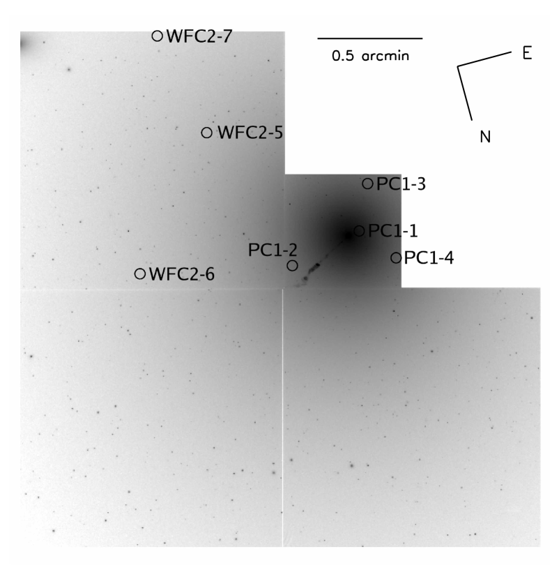
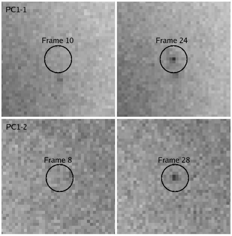
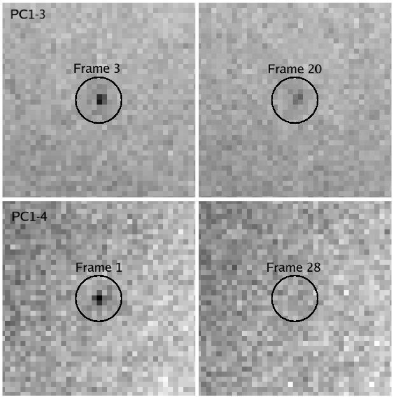
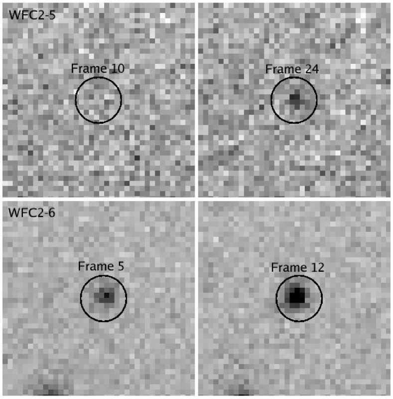
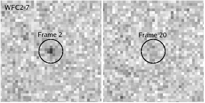
With a threshold , even with the hot pixel test applied, there are a number of ambiguous candidates. Among these there are the seven candidates that are clearly astrophysical. Increasing the threshold to removes most ambiguous detections, but allows all seven clear candidates. Thus, we will err on the side of conservatism and take the threshold to be . The candidates are listed in Table 2, along with their microlensing fit parameters in Table 3. A mosaic finder chart for the seven candidates is presented in Fig. 2. In Figs. 3-6 we illustrate the unsubtracted frames for the seven candidate events for both the baseline and the peak flux. Note that PC1-3 is a resolved source, and is visible in each frame before subtraction, and that WFC2-6 is coincident with a globular cluster.
4.7 First Interpretation of Candidates
Our primary science goal is to study microlensing populations around M87. With this aim, it is now appropriate to reject the candidates whose microlensing fits have low probability according to the distribution. Rejected events remain interesting as nova or variable candidates, as the microlensing template is a good generic bump finder. Non-microlensing bumps will pass all tests except that their microlensing fits will be unlikely. We require a within the usual confidence. For the 26 degrees of freedom appropriate for the microlensing fit, the requirement is . In fact the application of the lower limit does not exclude any events.
These variable sources have been selected in the F814W frames. They are now sought in the F606W frames, and approximate colors determined by simple aperture photometry. We can detect sources in F606W at the same or greater significance as F814W if or bluer.
The photometric fit parameters are listed in Table 3. Note that the flux excess is listed: this is the flux above the baseline of the microlensing fit. This excess flux is converted to magnitudes in the -band. Likewise, the color listed is the color of the excess flux. The lightcurves of the candidate events are plotted in Figs. 7-8. The fluxes in the two filters are plotted against each other in Fig. 9. Any microlensing event should exhibit a straight line on a flux-flux plot. Only candidates PC1-1 and WFC2-6 exhibit a significant color change. As we discuss next, these are likely to be novae.
Candidates PC1-1 and WFC2-6 are quite clearly novae, according to their magnitudes, colors and lightcurve shapes. Candidate WFC2-6 appears to be in a globular cluster of M87, and is discussed in more detail elsewhere (Shara et al. 2003). Candidates PC1-2 and WFC2-7 seem to be blue variables, possibly novae. Since their peaks are unobserved, it is hard to say more about them. Candidates PC1-3 and PC1-4 are redder variables, again with peak brightness unobserved. Candidate PC1-3 is in fact detected in all 30 visits. Candidate WFC2-5 is an excellent microlensing candidate, though its blue color is unexpected: red giants with are typically the most numerous sources.
Candidates PC1-3, PC1-4, WFC2-5, and WFC2-7 have an acceptable to be microlensing. However, only candidate WFC2-5 is sampled on both sides of the peak. Thus, while any of candidates PC1-3, PC1-4, WFC2-5, and WFC2-7 could be microlensing, only candidate WFC2-5 can be confidently proposed as a microlensing event. As a final criterion, we require that at least half of the half-width at half maximum be sampled on either side of the peak, thus only candidate WFC2-5 remains.
5 Detection Efficiency
Having developed the procedure for finding microlensing events in the dataset, we must now calculate the detection efficiency. We proceed in two ways. Starting at the level of event lightcurves, we thoroughly model the detection efficiency simply by generating a large number of artificial lightcurves with known event parameters and applying the lightcurve analysis, as described in §5.1. At the image level, artificial events are generated and put into the image stack. In this way the efficiency of the steps between the difference images and extracting lightcurves can be estimated, as described in §5.2. In the end, we will use the lightcurve efficiencies, with a correction derived by comparing with the artificial star efficiencies.
5.1 Lightcurve Tests
Calculating the detection efficiency using only a lightcurve test necessarily assumes that the noise model is perfect. We proceed with this assumption, but we will test it using artificial stars in §5.2.
A large number of theoretical lightcurves are generated, taking a grid over the interesting fit parameters: the peak significance , the timescale , and the minimum impact parameter (which has only a small effect on the shape of the lightcurve). Fixing these three parameters, lightcurves are generated with random values of the peak time , ranging over a generous interval containing the observation epochs. The fluxes at each epoch are taken from a Poisson distribution. These artificial lightcurves are then passed through the stages of baseline selection (§4.1), variability selection (§4.2) and lightcurve fitting (§4.3), identically to the lightcurves produced at each pixel in the result images. The fraction of artificial lightcurves, all representing “true” microlensing events, that pass all of these tests is then the detection efficiency for events with , and will be denoted . Results for some interesting fit parameters are plotted in Fig. 1.
5.2 Artificial Star Tests
As a check on the lightcurve detection efficiency of §5.1, we use an artificial star test. We randomly generate microlensing events and insert them in the existing image stack. This does in principle introduce a bias toward the large area of low surface brightness, but the event rate is expected to be only a weak function of surface brightness, so this prescription is adequate for our purposes. This artificial image stack is then processed identically to the true image stack. Some fraction of the artificial events are recovered. This fraction is the artificial star efficiency.
We focus on the WFC2 chip. Starting from just the artificial reference and difference images, the simplest test to be applied is the hot pixel test of §4.4. The probability that an artificial event is identified as a hot pixel can be determined. This analysis in fact provided guidance on how to construct the test so that there was a low probability of a false positive. We use three timescales: days, and eight peak flux levels corresponding to . For each combination, two thousand artificial events are generated. The events are randomly distributed uniformly in position on the chip and in peak time (between frame 1 and frame 30). Furthermore, they are uniformly distributed in sub-pixel offsets in units of 0.005″along each axis.
The expected flux of the artificial event is now determined from the theoretical lightcurve, which is in units of statistical significance. This is converted to expected flux simply by consulting the reference image to calculate the noise level. With the expected flux in each frame, multiplied by the normalized PSF, appropriately shifted, we compute the expected number of photons in each pixel due to the artificial event. The actual number for each pixel is generated according to a Poisson distribution. In this way for each artificial event, in each of the 30 frames, in each PSF pixel, we compute the number of photons due to the event. At each pixel position, we take the average over frames (neglecting frame 12) of the artificial event photons, and add this number to the reference image. This accounts for the fact that all events appear in the reference image at some level. We set a rough baseline for each event, and add or subtract the photons from the difference images.
From the artificial reference and difference images, the hot pixel test of §4.4 is applied. The probabilities of the artificial events being identified as hot pixels are plotted in Fig. 1. All of these probabilities are under 10%.
The hot pixel test is easy to apply as the optimally filtered result images are not required. To test the full pipeline, we proceed as follows. One thousand artificial events are generated similarly to the hot pixel test, with three timescales: days, and six peak flux levels corresponding to . The artificial events are divided roughly equally among the eighteen possibilities. These events are now randomly distributed in position as before.
With the artificial reference and difference images in hand, we proceed with the full analysis of §3 to produce optimally filtered result images. These artificial result images are then analyzed according to §4, with candidate events being selected. This analysis now includes the hot pixel test. Once the lightcurves are constructed, the analysis follows identically to §5.1. The artificial star efficiency so derived is plotted in Fig. 1.
5.3 Comparison of Efficiency Estimates
We now compare the two efficiency calculations. The artificial star calculation is in principle a more accurate estimate of the efficiency, but the lightcurve calculation is more computationally feasible. Thus, we proceed by checking the lightcurve efficiency with the artificial star efficiency for a few cases, and thus deriving a correction. The corrections to the lightcurve efficiencies are plotted in Fig. 1. These will be applied to and used in §6 to calculate the expected rate of detectable microlensing events.
6 Modeling of M87 and the Virgo Cluster
To interpret the results of this search for microlensing, we must have models for the lens populations along the line of sight to M87. The expected rate of microlensing events can be calculated from these models and the detection efficiencies calculated in §5. We will need the spatial and velocity distributions of sources (M87 stars) and lenses (M87 stars, MW halo objects, M87 halo objects, and Virgo cluster halo objects).
6.1 Microlensing Rate
The basic rate distribution for microlensing events can be expressed as the integral along the the line of sight of the lens density times the cross section (Griest 1991; Baltz & Silk 2000):
| (11) |
where , , is a modified Bessel function of the first kind, is the circular velocity of the lens population , and is the transverse velocity of the line of sight relative to the lens population (due to the motion of source and observer). This equation makes no mention of the detection efficiency, which is added as an integral over the minimum impact parameter :
| (12) |
Note that the fit parameters and have been replaced with more physical ones depending on . Here, is the naive (photon counting) significance with which the source star is detected if blending is ignored. Since is independent of , this rate can be written with an effective threshold value of , determined in the obvious manner,
| (13) |
and the threshold depends only on the event timescale and brightness of the source. To compute the total observed rate, the distribution is simply integrated over all , then integrated over the mass function of lenses and the luminosity function of sources. Note that in our dataset is unknown event by event, but integrating over all yields the total observed event rate. We could have just as easily studied the rate distribution as follows:
| (14) |
but it is more expensive computationally.
This discussion of rates has neglected finite source size effects. We include these effects using a simple prescription (Baltz & Silk 2000). For a given source flux, we can determine the required magnification to give a lensed flux that would satisfy the requirement of the consecutivity test. Finite source size effects imply a maximum magnification as a function of : as , the maximum magnification . We can solve for the largest allowing the required magnification, and truncate the integral in equation 11 accordingly. This means thats is now a function of , both because of the required magnification, but also in the source radius as a function of brightness.
It is interesting to point out the relationship between microlensing rate and stellar population, first argued by Gould (1995). All other quantities being equal, the microlensing rate is roughly proportional to the surface brightness fluctuation flux , where the average is over the luminosity function of source stars. From equation 13, we can argue that since the impact parameter is inversely proportional to the magnification for large magnifications (the relevant regime here), then brighter stars allow linearly proportionally larger values of , keeping the signal-to-noise ratio at event peak fixed. Furthermore, these events are also observable for longer ( is longer), again proportional to source flux. Thus the rate is proportional to , yielding the surface brightness fluctuation flux when integrated over the luminosity function. This relation is of course affected by finite source size effects, as the maximum magnification will depend on stellar radii.
These rates assume a maxwellian velocity distribution of lenses with uniformly moving sources. If the source velocities are also maxwellian (as should be approximately the case for an elliptical galaxy), the extra velocity integrals can be separated out. The final outcome is the same if the identification is made.
6.2 Surface Brightness Profile and M87 Stars
The surface brightness profile of M87 has been well studied by numerous authors. We will construct a composite profile from several studies that extend from to more than . Within 20″of the center of M87, we use the -band surface brightness profile of Lauer et al. (1992). We use the profile from Young et al. (1978) to extend to 80″. At the largest radii, out to 150″, we use the -band results of Peletier et al. (1990). These three measurements are spliced together, and fit with a smoothly broken power law whose error is less than mag arcsec-2 in the range , given by
| (15) |
in mag arcsec-2, where governs the speed of the power law break, are the inner and outer power law slopes, and are normalization constants. Note that gives a standard broken power law, with break at . At very small and very large radii, this reduces to a single power law: .
The fit to the surface brightness profile is smooth, and thus we can perform an Abel inversion under the assumption that the system is spherically symmetric. For convenience, we define the 2-d luminosity density . Taking its derivative, we can write down the 3-d luminosity density,
| (16) |
This yields a luminosity density for M87, in mag arcsec-3, which we can apply to microlensing simulations. The Abel inversion is done numerically, yielding a table of density values. This table is again fit to a smoothly broken power law. The fit constants are , , . This fit has errors less than mag arcsec-3 in the range . To arrive at a mass density, we assume that the -band mass to light ratio is 4.0 .
We assume that the velocity distribution of M87 stars is maxwellian, with 1-d velocity dispersion km s-1. Furthermore we assume that it is isotropic, so radial and tangential dispersions are the same.
6.3 Milky Way Halo
We will use simple models for the dark halos of each relevant object. The isothermal sphere with core has an asymptotic density profile, giving a flat rotation curve. The lack of observed central density cusps indicates that a core is appropriate. The density of lenses making up a fraction of the dark halo is given by
| (17) |
where km s-1 is the asymptotic rotation speed of the Milky Way. We will take a core radius kpc, though the value doesn’t much matter as the line of sight to M87 is nearly perpendicular to the Milky Way disk. The velocity distribution of the halo is taken to be maxwellian, with a circular velocity equal to , making km s-1. We impose a cutoff at a distance of 200 kpc from the center.
6.4 M87 Halo
For M87 we will also use an isothermal sphere with a core. We will vary the core radius, taking kpc as the fiducial value. We assume a 1-d velocity dispersion km s-1, giving km s-1. Based simply on dispersion velocity, M87 is roughly five times as massive as the Milky Way. We allow the halo lens fraction to be independent of .
6.5 Virgo Cluster Halo
The halo of the Virgo cluster is more problematic. Again, we will assume an isothermal sphere with a core, with km s-1 ( km s-1). We will assume that M87 is centered in the Virgo halo. This approach requires that we assign a very large core radius to the Virgo halo: for as small as 100 kpc, Virgo dominates at a radius of 40 kpc from the center of M87. Again, we allow an independent halo lens fraction .
6.6 Expected Event Rates
Armed with the model for M87 and the Virgo cluster, we can now proceed to compute the expected rate of detectable microlensing events. Some experimental parameters are required. Furthermore, we must make assumptions about the luminosity function of M87 stars, and about the mass function of the lenses.
The capabilities of the WFPC2 can be summarized for our purposes as follows. We assume that the zero point in F814W is mag in the -band (this flux gives one photo-electron per second), and that only the F814W frames are used to detect events: namely an exposure of s = 1040 s per orbit. The zero point for this exposure time is mag, giving one photo-electron over the exposure. The resolution can be characterized by one number per chip, , where is the normalized PSF (Gould 1996). Measured in pixels (taking (0.0455 arcsec)2 for PC1 and (0.1 arcsec)2 for WFC2, WFC3, WFC4), the PSF sizes are 20.0, 7.31, 9.05, 7.89 for the PC1, WFC2, WFC3, and WFC4, respectively. These are somewhat less than 0.1 arcsec2. Lastly, we assume that the read noise is 5 photoelectrons, and that the dark noise is negligible.
We assume that the source population is circularly symmetric, with surface brightness taken from §6.2. We take the background sky brightness to be a uniform mag arcsec-2 in the -band. We will compute the microlensing rate at radial positions spaced by 1 arcsec, starting 1 arcsec from the center of M87 and extending to 200 arcsec. The two-dimensional microlensing rate is trivially constructed from this.
The surface brightness serves to normalize the luminosity function for stars in M87. We assume that M87 has the same luminosity function found for the Galactic bulge by Terndrup, Frogel & Whitford (1990). We adjust the high-luminosity cutoff to give a surface brightness fluctuation magnitude of , appropriate for M87. Taking a distance modulus of to the Virgo cluster, we can express the signal-to-noise ratio to detect a star of absolute magnitude magnified by a factor ,
| (18) |
Lastly, we fix the mass functions for both the stellar component of M87, and for the lenses. We take the Chabrier (2001) mass function for stars, which has an effective peak around 0.1 . For the lenses, we take a delta function at dex solar (0.32), similar to the best value found by the MACHO collaboration (Alcock et al. 2000).
We now have a complete model for calculating the microlensing event rate. We use thresholds of and 100, and we vary the core radii of both the M87 and Virgo cluster halos. The results are summarized in Table 4, clearly showing the dependence on core radii and on lens fractions , and .
From these simulations of microlensing in this dataset, we conclude that of order 10 events are expected for . Taking as indicated by MACHO (Alcock et al. 2000), we expect 1–2 events with the sensitivity to microlensing that we were able to achieve, namely .
7 Discussion
We have identified seven candidate variable point sources in M87. The obvious question is what are these sources. We will discuss several possibilities below. If any of these candidates are in fact due to microlensing, we want to understand the implications for populations of lenses associated with the Virgo Cluster.
Perhaps most obviously, any of these candidate events could potentially be classical novae, with the exception of PC1-3 which is far too red. A study of these candidates as novae will be reported elsewhere (Shara et al. 2003). How many novae might we expect to see in M87 during a 30 day run? A simple, purely theoretical estimate is as follows. The space density of cataclysmic variables (CVs) near the Sun is roughly that of all stars. All CVs undergo thermonuclear runaways – nova eruptions – when their white dwarf accretes enough hydrogen-rich matter (typically ) from the main sequence companion. The accretion timescale (and hence inter-eruption timescale) is often of order to years. If the CVs in M87 are similar to those in the solar neighborhood, then there should be CVs among the stars of M87. Thus we expect 100-1000 nova eruptions/year in M87, or 10-100 nova eruptions in M87 during a month-long survey. As we are almost certainly not complete in our detections of low luminosity novae, or those located close to the galaxy’s nucleus, the likely/possible novae we do observe are in good agreement with the simple prediction.
Candidate PC1-3 is likely to be a Mira variable. From the lightcurve it appears to vary by at least 2 magnitudes, but Miras can exhibit variations much larger than this. Candidate PC1-4 is our second reddest, but it is fairly blue to be a Mira. However, Miras are known to be bluer at maximum light (Kanbur, Hendry & Clarke 1997), so it is not unreasonable to suppose this might also be a Mira.
From its shape, candidate WFC2-5 is an excellent microlensing candidate. In addition, its color is quite constant throughout the time series. However, we can not rule out the possibility that it is a nova. Its blue color is certainly consistent with the nova hypothesis. In fact for it to be microlensing the source would have to be e.g. a horizontal branch star. On numbers alone, we expect that most microlensing events will be red giants, so this is puzzling. Since the horizontal branch lies at for , the implied magnification for WFC2-5 is roughly 620. From the full-width at half maximum timescale days, the implied Einstein time is days. The peak of the distribution is at roughly 75 days for typical stellar mass lenses. This implies that a source 3.8 magnitudes brighter than the horizontal branch is typical. This is near the tip of the red giant branch. In other words, we expect most events to be much lower magnifications of much brighter stars. This seems to indicate that the horizontal branch microlensing hypothesis is disfavored. We note that this source is much brighter than the aperiodic blue variables, otherwise known as blue bumpers, observed by the MACHO collaboration (Keller et al. 2002). Such sources vary by less than 0.5 magnitudes, at .
We have performed a simple test for the presence of finite source effects in candidate WFC2-5. Following Yoo et al. (2004), we introduce one more fit parameter, the angular size of the source relative to the Einstein angle: . With impact parameter in Einstein units as before, we define , , and thus . The degenerate microlensing lightcurve with finite source effects is now
| (19) |
with being the new fit parameter (since is already fit for with and ; see equations 8 and 9), and for simplicity we assume no limb darkening. Note that is the elliptic integral of the second kind. We find a new best fit, with magnitudes, days, days, and . This fit implies a much larger (20.5x) naive magnification, and much shorter (25.1x) naive timescale. The minimum impact parameter is roughly 1/30 of the stellar radius, namely the finite source effects are severe. The fit is not overwhelmingly better; it is slightly wider and flatter near the peak. A simple -test indicates that finite source effects exist at 87% confidence. However, the higher magnification implied by the finite source fit is less likely by a factor of 20. For a horizontal branch star, , implying . Taking , and a solar mass lens, kpc. This is reasonable for an M87 halo lens, but probably not for an M87 star. Returning to the fit without finite source size effects, for the horizontal branch source. Starting with this fit, and computing as a function of , we find that is pretty flat as a function of for , but that it blows up for (by this we mean that goes from 2 at to 5 at ). Enforcing the condition that for the horizontal branch star requires that , implying kpc for a solar mass lens. Again, this would require an M87 halo or Virgo halo lens.
Considering the microlensing hypothesis, we would expect to detect 1-2 microlensing events from a 20% microlensing halo for the Virgo cluster with the sensitivity level achieved. Having one solid candidate is certainly consistent with that, though even in the case of zero candidates, the limits we might place on the Virgo lens fraction are not strong: naively the 95% confidence limit on the lens fraction is .
We have shown that it is possible to detect variables near the photon noise limit with repeat observations using HST. In the future, a continuation of this work using the much more sensitive Advanced Camera for Surveys (ACS) would allow a huge increase in sensitivity to microlensing. Firstly, the area covered is twice as large, second the efficiency is 4.5 times higher in the -band, and third, is a factor of 1.6 smaller. These factors combined allow a factor of fourteen increase in sensitivity for the same time coverage. Clearly this is a huge advantage, meaning a 20% Virgo halo would contribute more like 15-30 events in a one-month program. In addition, we believe that the sensitivity could be made significantly higher by altering the pointing by several PSF diameters from visit to visit, allowing a complete decoherence between source and detector structure, thus removing essentially all hot pixels from the type of variability search we performed. Allowing a lower threshold would obviously be a significant improvement.
We have reported on microlensing candidates observed toward M87. We have shown that the HST is a powerful tool for this kind of science. The improvements that would be allowed by the ACS are striking, and would definitively detect, or rule out at high confidence, a microlensing halo around the Virgo cluster.
References
- (1)
- (2) Alcock, C. et al. 2000, ApJ, 542, 281
- (3)
- (4) Afonso, C. et al. 2003, A&A, 400, 951
- (5)
- (6) Ansari, R., et al. 1999, A&A, 344, L49
- (7)
- (8) Aurière, M., et al. 2001, ApJ, 553, L137
- (9)
- (10) Baillon, P., Bouquet, A., Giraud-Héraud, Y., & Kaplan, J. 1993, A&A, 277, 1
- (11)
- (12) Baltz, E. A. & Silk, J. 2000, ApJ, 530, 578
- (13)
- (14) Calchi Novati, S., et al. 2002, A&A, 381, 848
- (15)
- (16) Castleman, K. R. 1995, “Digital Image Processing,” (Prentice Hall)
- (17)
- (18) Chabrier, G. 2001, ApJ, 554, 1274
- (19)
- (20) Crotts, A. P. S. 1992, ApJ, 399, L43
- (21)
- (22) Crotts, A. P. S. & Tomaney, A. B. 1996, ApJ, 473, L87
- (23)
- (24) Einstein, A. 1936, Science, 84, 506
- (25)
- (26) Gondolo, P. 1999, ApJ, 510, L29
- (27)
- (28) Gould, A. 1995, ApJ, 455, 44
- (29)
- (30) Gould, A. 1996, ApJ, 470, 201
- (31)
- (32) Griest, K. 1991, ApJ, 366, 412
- (33)
- (34) de Jong, J. T. A., et al. 2003, A&A, in press, astro-ph/0307072.
- (35)
- (36) Kanbur, S. M., Hendry, M. A. & Clarke, D. 1997, MNRAS, 289, 428
- (37)
- (38) Keller, S. C., Bessell, M. S., Cook, K. H., Geha, M., & Syphers, D. 2002, AJ, 124, 2039
- (39)
- (40) Lauer, T. R., et al. 1992, AJ, 103, 703
- (41)
- (42) Lauer, T. R. 1999, PASP, 111, 227
- (43)
- (44) Lauer, T. R. 1999, PASP, 111, 1434
- (45)
- (46) Paulin-Henriksson, S. et al. 2003, A&A, 405, 15
- (47)
- (48) Peletier, R. F., Davies, R. L., Illingworth, G. D., Davis, L. E. & Cawson, M. 1990, AJ, 100, 1091
- (49)
- (50) Riffeser, A., Fliri, J., Bender, R., Seitz, S. & Goessl, C. A. 2003, ApJ, 599, L17
- (51)
- (52) Shara, M. M., Zurek, D. R., Baltz, E. A., Lauer, T. R. & Silk, J. 2003, in preparation
- (53)
- (54) Terndrup, D. M., Frogel, J. A., & Whitford, A. E. 1990, ApJ, 357, 453
- (55)
- (56) Uglesich, R. 2001, Ph.D. thesis, Columbia University
- (57)
- (58) Uglesich, R., Crotts, A. P. S., Baltz, E. A., de Jong, J., Boyle, R. P. & Corbally, C. J., 2003, in preparation
- (59)
- (60) Yoo, J. et al. 2004, ApJ, in press, astro-ph/0309302
- (61)
- (62) Young, P. J., Westphal, J. A., Kristian, J., Wilson, C. P., Landauer & F. P. 1978, ApJ, 221, 721
- (63)
| Visit | Date | Date | Dataset | |||
|---|---|---|---|---|---|---|
| (GMT) | (MJD) | (days) | ( pixels) | |||
| 1 | May 28 2001 | 52057.430729 | 0.00 | 0.00 | 0.00 | U6730101R-5R |
| 2 | May 29 2001 | 52058.366840 | 0.94 | 0.05 | 0.08 | U6730201R-5R |
| 3 | May 30 2001 | 52059.303645 | 1.87 | 1.07 | 0.10 | U6730301R-5R |
| 4 | May 31 2001 | 52060.239756 | 2.81 | 0.93 | 0.56 | U6730401R-5R |
| 5 | June 1 2001 | 52061.243229 | 3.81 | 1.02 | -0.67 | U6730501R-5R |
| 6 | June 2 2001 | 52062.313367 | 4.88 | 1.01 | -1.02 | U6730601R-5R |
| 7 | June 3 2001 | 52063.383506 | 5.95 | 0.01 | -0.88 | U6730701R-5R |
| 8 | June 4 2001 | 52064.453645 | 7.02 | -0.31 | 0.40 | U6730801R-5R |
| 9 | June 5 2001 | 52065.389756 | 7.96 | -0.05 | 0.36 | U6730901R-5R |
| 10 | June 6 2001 | 52066.326562 | 8.90 | 0.05 | 0.03 | U6731001R-5R |
| 11 | June 7 2001 | 52067.262673 | 9.83 | 1.06 | 0.03 | U6731101R-5R |
| 12 | June 8 2001 | 52068.333506 | 10.90 | 1.15 | 0.59 | U6731201R-5R |
| 13 | June 9 2001 | 52069.269618 | 11.84 | 1.05 | -0.50 | U6731301R-5R |
| 14 | June 10 2001 | 52070.210590 | 12.78 | 1.12 | -0.61 | U6731401R-5R |
| 15 | June 11 2001 | 52071.145312 | 13.71 | 0.27 | -1.40 | U6731501R-5R |
| 16 | June 12 2001 | 52072.147395 | 14.72 | 0.16 | -1.16 | U6731601R-5R |
| 17 | June 13 2001 | 52073.218229 | 15.79 | -0.02 | 0.34 | U6731701R-5R |
| 18 | June 14 2001 | 52074.152951 | 16.72 | 0.01 | 0.21 | U6731801R-5R |
| 19 | June 15 2001 | 52075.093229 | 17.61 | 1.07 | 0.24 | U6731901R-5R |
| 20 | June 16 2001 | 52076.027951 | 18.60 | 1.09 | 0.11 | U6732001R-5R |
| 21 | June 16 2001 | 52076.961979 | 19.43 | 1.10 | -0.76 | U6732101R-5R |
| 22 | June 18 2001 | 52078.032812 | 20.60 | 1.13 | -0.80 | U6732201R-5R |
| 23 | June 19 2001 | 52079.103645 | 21.67 | -0.01 | -0.76 | U6732301R-5R |
| 24 | June 20 2001 | 52080.039062 | 22.61 | 0.17 | -0.96 | U6732401R-5R |
| 25 | June 21 2001 | 52080.978646 | 23.61 | 0.03 | 0.44 | U6732501R-5R |
| 26 | June 22 2001 | 52081.982118 | 24.61 | 0.01 | 0.38 | U6732601R-5R |
| 27 | June 23 2001 | 52082.984896 | 25.62 | 1.24 | -0.06 | U6732701R-5R |
| 28 | June 24 2001 | 52084.052257 | 26.62 | 1.16 | 0.05 | U6732801R-5R |
| 29 | June 25 2001 | 52085.055034 | 27.62 | 1.06 | -0.69 | U6732901R-5R |
| 30 | June 25 2001 | 52085.993923 | 28.56 | 1.32 | -1.16 | U6733001R-5R |
Note. — The date refers to that of the first observation in a given visit. Each visit comprises four dithered F814W images, followed by a single F606W image. Offsets are shown for CCD WFC2 only in units of subpixels relative to the origin of the first visit.
| number | pixel (fit) | pixel (flux) | radius | comments | |||||
|---|---|---|---|---|---|---|---|---|---|
| (arcsec) | (J2000) | (J2000) | |||||||
| PC1-1 | 530 | 439 | 528.6 | 438.6 | 3.5 | 12 30 49.744 | 12 23 29.39 | classical nova | |
| PC1-2 | 102 | 216 | 101.0 | 214.6 | 17.4 | 12 30 48.285 | 12 23 31.13 | rising | |
| PC1-3 | 586 | 742 | 585.3 | 741.5 | 16.4 | 12 30 50.262 | 12 23 17.73 | declining | |
| PC1-4 | 767 | 267 | 766.8 | 265.9 | 17.4 | 12 30 50.204 | 12 23 40.88 | declining | |
| WFC2-5 | 507 | 255 | 505.9 | 254.4 | 49.2 | 12 30 47.684 | 12 22 46.32 | microlensing candidate | |
| WFC2-6 | 94 | 449 | 93.6 | 448.4 | 61.4 | 12 30 45.408 | 12 23 16.17 | globular cluster nova | |
| WFC2-7 | 788 | 399 | 787.6 | 398.5 | 78.3 | 12 30 47.557 | 12 22 14.89 | declining | |
Note. — Final candidate list passing all cuts. Pixel coordinates are given, both as the center pixel of the group that passes all cuts, and as a flux–weighted centroid. One event is an excellent microlensing candidate, well sampled on both sides of the peak. Two candidates are obvious novae. The remainder are probably variable stars. Note that only the PC1 and the WFC2 chips had candidates passing all cuts.
| number | peak | dof | comments | ||||
|---|---|---|---|---|---|---|---|
| (days) | (MJD) | (frame) | |||||
| PC1-1 | -8.85 | 1.36 | 23.58 | 24 | 3.18 | classical nova | |
| PC1-2 | -7.41 | 16.4 | 26.15 | 28 | 2.13 | rising | |
| PC1-3 | -7.97 | 19.7 | 2.94 | 3 | 1.02 | declining | |
| PC1-4 | -7.37 | 7.11 | -0.28 | 1 | 0.74 | declining | |
| WFC2-5 | -6.73 | 7.02 | 23.26 | 24 | 1.23 | microlensing candidate | |
| WFC2-6 | -8.09 | 0.91 | 11.58 | 12 | 3.67 | globular cluster nova | |
| WFC2-7 | -6.49 | 11.6 | -0.69 | 2 | 1.43 | declining |
Note. — Microlensing fit parameters for final candidates. These are the maximum flux increase expressed in absolute magnitude (taking ), the full-width at half maximum , peak time as MJD = Modified Julian Date 52057, frame with maximum flux (1-30), color of the excess flux (obtained with aperture photometry), and the goodness of the microlensing fit. For WFC2-5, the only event with both good coverage of the peak and a good microlensing fit, the fit errors are: magnitudes, days, days. Errors on the fit parameters of the other events are much less meaningful.


| threshold | |||||
|---|---|---|---|---|---|
| M87 stars | 0.55 | 0.22 | |||
| Milky Way Halo | 0.32 | 0.19 | |||
| M87 Halo | kpc | 2.65 | 1.32 | ||
| kpc | 2.38 | 1.21 | |||
| kpc | 2.02 | 1.06 | |||
| Virgo Halo | kpc | 14.2 | 8.03 | ||
| kpc | 10.5 | 6.13 | |||
| kpc | 5.91 | 3.60 | |||
| Totals | (9—18) | (5—10) |
Note. — Expected number of microlensing events for each component of the model. The self lensing component is quite small, less than 0.25 events expected. The dominant component is clearly the Virgo cluster halo. For , the M87 halo contribution is comparable to the self lensing. The Milky Way halo contribution is quite small, and with , it is much less than even the self lensing component.