Simulating Chandra observations of galaxy clusters

Abstract

Numerical hydro-N-body simulations are very important tools for making theoretical predictions for the formation and evolution of galaxy clusters. Their results show that, accordingly with recent Chandra and XMM-Newton observations, the atmospheres of clusters of galaxies have quite complex angular and thermal structures, far from being spherically symmetric. In many cases the full understanding of the physical processes behind these features can be only achieved by direct comparison of observations to hydro-N-body simulations. Although simple in principle, these comparisons are not always trivial. In fact, real data are convolved with the instrument response and are subject to both instrumental and sky background which may substantially influence the apparent properties of the studied features. To overcome this problem we build the software package X-MAS (X-ray MAp Simulator) devoted to simulate X-ray observations of galaxy clusters obtained from hydro-N-body simulations. One of the main feature of our program is the ability of generating event files following the same standards used for real observations. This implies that our simulated observations can be analysed in the same way and with the same tools of real observations. In this paper we present how this software package works and discuss its application to the simulation of Chandra ACIS-S3 observations. Using the results of high-resolution hydro-N-body simulations, we generate the Chandra observations of a number of simulated clusters. We compare some of the main physical properties of the input data to the ones derived from simulated observations after performing a standard imaging and spectral analysis. We find that, because of the background, the lower surface brightness spatial substructures, which can be easily identified in the simulations, are no longer detected in the actual observations. Furthermore, we show that, if the thermal structure of the cluster along a particular line of sight is quite complex, the projected spectroscopic temperature obtained from the observation is significantly lower than the emission-weighed value inferred directly from hydrodynamical simulation. This implies that much attention must be paid in the theoretical interpretation of observational temperatures.

1 Introduction

Theoretical studies of the dynamical processes underlying the formation and evolution of galaxies and galaxy clusters are now mainly based on the results of numerical hydro-N-body simulations. Since the pioneering attempts of solving simple N-body problems in the early ’70s, nowadays simulation codes have dramatically improved. Besides the gas hydrodynamics, their most recent versions may account for some complex physical processes, that include, but are not limited to, gas cooling and heating, star formation and feedback, thermal conduction, magnetic fields (see, e.g., Lewis et al. 2000; Yoshida et al. 2002; Muanwong et al. 2002; Dolag, Bartelmann & Lesch 2002; Marri & White 2003; Kay, Thomas & Theuns 2003; Springel & Hernquist 2003; Tornatore et al. 2003; Borgani et al. 2003). Simulation results clearly show that, during their evolution, clusters of galaxies experience violent events that release an enormous amount of energy in the intracluster medium (ICM). These events induce strong, but transient, variation of both ICM density and temperature, so that their distribution is far to be smooth and spherical symmetric.

From the observational side, thanks to the superb angular and spectral resolution of the latest generation X-ray satellites, Chandra and XMM-Newton, we now know that many galaxy clusters, including the ones previously identified as relaxed, actually present a great deal of spatial features and have a rather complex thermal structure. Some of these include cold fronts (see, e.g., Abell 2142, Markevitch et al. 2000; Abell 3667, Vikhlinin, Markevitch & Murray 2001; RX J1720+26, Mazzotta et al. 2001; A1795, Markevitch, Vikhlinin & Mazzotta 2001; 2A 0335+096, Mazzotta, Edge & Markevitch 2003), X-ray cavities (i.e. Hydra A, McNamara et al. 2000; Perseus, Fabian et al. 2000; Abell 2052, Blanton et al. 2001; Abell 2597, McNamara et al. 2001; MKW3s, Mazzotta et al. 2002b; RBS797, Schindler et al. 2001; Abell 2199, Johnstone et al. 2002; Abell 4059, Heinz et al. 2002; Virgo, Young, Wilson & Mundell 2002; Centaurus, Sanders & Fabian 2002; Cygnus A, Smith et al. 2002), X-ray blobs and/or filaments (see, e.g., Abell 1795, Fabian et al. 2001; Abell 3667, Mazzotta, Fusco-Femiano & Vikhlinin 2002a; 2A 0335+096, Mazzotta et al. 2003). Furthermore, recent observations indicate that also the gas metal content may have a rather complex distribution that may lead to what we observe as an off-centre peaked metallicity profile (see, e.g., Persueus, Schmidt, Fabian & Sanders 2002, and Churazov et al. 2003; Centaurus, Sanders & Fabian 2002; 2A 0335+096, Mazzotta et al. 2003). Due to their complex nature and the impossibility of using simple deprojection techniques, most of these observed features can be quantitatively studied only through a direct comparison to numerical simulations. Ideally, to make these comparisons straightforward one needs to re-process the simulations themselves through a sort of virtual observatory in such a way that the information provided is as much as possible similar to what an observer can obtain through real X-ray observations of clusters.

In this paper we present X-ray MAp Simulator (X-MAS), a software package we developed to simulate X-ray observations of galaxy clusters obtained from hydro-N-body simulations. The main characteristic of our code is that, giving as input any hydro-N-body simulation, it produces as output an event file which is completely similar to what an X-ray observer would obtain from a real observation. This means that the simulated data can be analysed in the same way and using the same tools of real observations. For the moment our software package simulates ACIS-S3 Chandra observations only. In the future we will extend the code to simulate Chandra in the ACIS-I mode and XMM-Newton observations with both EPIC and MOS detectors.

The outline of the paper is as follow. In Section 2 we present the general characteristics of X-MAS. In Section 3 we show the results of a simulation of an ACIS-S3 observation of a galaxy cluster. In Section 4 we discuss the possible discrepancy between the projected temperature derived from the spectral analysis of the observation and the emission-weighted temperature directly obtained from the hydro-N-body simulation. In Section 5 we show some applications of X-MAS, namely temperature profiles and maps. Finally in Section 6 we give our conclusions.

2 X-ray MAp Simulator: The method

In this section we describe how the X-MAS package works. The package can be divided into two main units. The first unit is quite general and does not depend on the specific characteristics of the X-ray telescope. For each considered energy channel, it generates a corresponding map of the differential flux obtained by projecting the specific emission of each particle along the line of sight. The resulting information for the angular position and energy is stored in a three-dimensional array. An equivalent way to describe the task of this first unit is to say that, for each line of sight within a defined field of view, it calculates and stores the corresponding projected mass-weighted spectrum. The second unit takes each spectrum calculated by the first one and simulates the data relevant to an observation with a specific X-ray telescope and detector for a defined amount of time. Of course, this second unit strongly depends on the characteristics of the X-ray telescope and detector we consider. At present our software package simulates Chandra observations in ACIS-S3 configuration only. The application of our simulation package to simulate Chandra in the ACIS-I mode and XMM-Newton observations with both EPIC and MOS detectors requires an adaptation of this second unit only. In the following we describe in details how the two package units work.

2.1 First Unit: generating differential flux maps

The first unit of our package X-MAS requires as input the output of an hydro-N-body simulation. After selecting the direction and the depth of the galaxy cluster for which we want to simulate the observation, the program generates the cluster projected spectra corresponding to all the lines of sight in a defined field of view. This is simply done by considering an energy interval $[E_{\rm min},E_{\rm max}]$, which we divide in $n_{{}_{E}}$ regular energy channels with energy width $\Delta E=(E_{\rm max}-E_{\rm min})/n_{{}_{E}}$. The energy interval and the energy resolution selected for unit one of the program need to be higher than or equal to the energy response and the energy resolution of the instrument we intend to simulate later with unit two, respectively. We use $E_{\rm min}=0.1$ keV, $E_{\rm max}=10$ keV and $n_{{}_{E}}=495$ (or equivalently $\Delta E=20$ eV).

For each of these channels we calculate the two-dimensional map of the corresponding differential flux produced by the simulated galaxy cluster simply by projecting on a regular grid (1024 pixels $\times$ 1024 pixels) the flux $F^{\nu}_{i}$ of each particle and summing over all particles. The differential flux for the cluster is finally stored in a three-dimensional array in which two dimensions represent the angular coordinates and the third one is for the energy.

In order to calculate the flux associated with each particle we follow a procedure very similar to the one described in Mathiesen & Evrard (2001). Starting from its three-dimensional position ${\bf{x}}_{{}_{i}}$, mass $m_{i}$ and density $\rho_{i}$, we assign to the $i$-th gas particle in the simulation an effective volume $V_{i}=m_{i}/\rho_{i}$, which is assumed for simplicity to be cubic and centred on ${\bf{x}}_{{}_{i}}$.

For cosmological sources, the standard relation between flux $F$ and luminosity $L$ holds: $F={L/4\pi d_{L}^{2}}$, where $d_{L}$ is the luminosity distance (depending on cosmology and on the source redshift $z$). Considering differential quantities, the previous relation becomes $F_{\nu}=[{(1+z)L_{\nu(1+z)}]/4\pi d_{L}^{2}}$, where the ${\nu}$ pedex accounts for the dependence on the energy band. If the flux is expressed in terms of incoming photons instead of energy, we can introduce the quantity $F_{\nu}^{\gamma}\equiv{F_{\nu}/h\nu}$ (in photon/s/cm²/keV), so that $F_{\nu}^{\gamma}d(h\nu)$ represents the flux of the incoming photons with energy in the range $[h{\nu},h({\nu+d\nu})]$ keV. In general, we prefer to give quantities like luminosity or flux in terms of incoming photons or counts (instead of energy) because they can be more easily related to real observational data. Finally the relation between flux and luminosity simply becomes

$$F_{\nu}^{\gamma}={(1+z)^{2}L_{\nu(1+z)}^{\gamma}\over 4\pi d_{L}^{2}}\ .$$ (1)

The emissivity per unit of frequency $\epsilon_{\nu}$ in a region of volume $V$ is related to the luminosity as $L_{\nu}=\int_{V}\epsilon_{\nu}\,dV^{\prime}$; a similar relationship holds for differential and photon quantities.

For a galaxy cluster the emissivity from a small enough region of plasma is given by a single temperature thermal model. Given the electron and hydrogen densities ($n_{e}$ and $n_{{}_{H}}$, respectively), the emissivity can be written as $\epsilon=n_{e}n_{{}_{H}}\,P(T,Z)$. The quantity $P(T,Z)$ is usually called power coefficient and depends only on the temperature $T$ and metallicity $Z$ of the gas. Using the relation above, the photon luminosity can be written as $L_{\nu}^{\gamma}=\int_{V}\epsilon_{\nu}^{\gamma}\,dV^{\prime}=P_{\nu}^{\gamma}EM$; the quantity $EM\equiv\int_{V}n_{e}n_{{}_{H}}dV^{\prime}$ is often referred to as emission measure. The final relation between flux and power coefficients is then

$$F_{\nu}^{\gamma}={(1+z)^{2}\over 4\pi d_{L}^{2}}EM\,P_{\nu(1+z)}^{\gamma}(T,Z)\ .$$ (2)

Using the temperature and the metallicity of each particle in the simulation, we calculate $P(T_{i},Z_{i})$ using the single temperature thermal model mekal (see, e.g., Kaastra & Mewe 1993; Liedahl, Osterheld & Goldstein 1995, and references therein) implemented in the utility XSPEC (Arnaud 1996).

To make our simulator of X-ray observation more complete, we allow to include the effects on the spectra induced by the Galactic HI absorption. This is done, at the end of the procedure, by multiplying the flux in each energy channel by an absorption coefficient given by the wabs model (Morrison & McCammon 1983), once a value for the column density $N_{{}_{H}}$ is assumed.

2.2 Second Unit: Simulating Chandra ACIS-S3 observations

The second unit of our simulation package X-MAS takes as input the projected spectra produced by the first unit and, after convolving them with the technical characteristics of a specific instrument, generates an event file similar to the one obtained from a real observation. To do that we use the data simulation command fakeit in the utility XSPEC (see, e.g., Xspec User’s Guide version 11.2.x; Dorman & Arnaud 2001). The above command creates simulated data from the input spectral model by convolving it with the ancillary response files (ARF) and the redistribution matrix files (RMF), which fully define the response of the considered instrument, and by adding noise appropriate to the specified integration time. Once the data of all spectra have been simulated, we generate a photon event file satisfying the standards defined for real observations. This is quite important because it allows our mock observations to be analysed by using the same tools and procedures used for the real ones.

In the following we describe how we use the second unit of our software package to simulate X-ray observations performed using Chandra with the back illuminated CCD ACIS-S3.

The ACIS-S3 detector is a square with a grid of 1024 pixels $\times$ 1024 pixels, and a field of view of about 8.3 arcmin by side. The nominal angular resolution is about 0.5 arcsec/pixel. Although the instrumental response is position-dependent, it is quite constant over CCD subregions of $32\times 32$ pixels, which for convenience we call detector tiles (or tiles for short). To fully account for the instrument response the Chandra calibration team produced 1024 ARF and 1024 RMF, one for each of the detector tile above.

Detection events have to preserve the spatial and spectral information. As explained above, their number and energy are obtained by executing the command fakeit of the utility XSPEC using the appropriate ARF and RMF. To account for the instrumental background we provide to the fakeit command an appropriate background file extracted from the blank-sky background dataset (Markevitch 2001) in the same tile subregion corresponding to the spectrum to be simulated.

To speed up the simulation process we use an adaptive algorithm: before simulating the data of each spectrum, we estimate the expected number counts associated with each detector tile. If this number is lower than a given threshold we generate the events, otherwise we iteratively subdivide the region in four squares, until the threshold is reached. The spatial position of the events obtained in this way is then reconstructed by randomly distributing the simulated photons inside the region by using a weight proportional to the original flux.

3 ACIS-S3 observation of a simulated cluster

As a first example of possible applications of our software package, we generate a 300 ks Chandra ACIS-S3 observation of a high-resolution hydro-N-body simulation of a galaxy cluster. The object was selected from a sample of 17 objects obtained using the technique of re-simulating at higher resolution a patch of a pre-existing cosmological simulation. The assumed cosmological framework is a cold dark matter model in a flat universe with a present matter density parameter $\Omega_{m}=0.3$ and a contribution to the density due to the cosmological constant $\Omega_{\Lambda}=0.7$; the baryon content corresponds to $\Omega_{B}=0.03$; the value of the Hubble constant (in units of 100 km/s/Mpc) is $h=0.7$, and the power spectrum normalization is given by $\sigma_{8}=0.9$. The re-simulation method, called ZIC (for Zoomed Initial Conditions), is described in detail in Tormen, Bouchet & White (1997), while an extended discussion of the properties of the whole sample of these simulated clusters is presented elsewhere (Tormen, Moscardini & Yoshida 2003; Rasia, Tormen & Moscardini 2003). Here we remind only some of the characteristics of the cluster used in this paper. It has been obtained by using the publicly available code GADGET (Springel, Yoshida & White 2001); during the run, starting at redshift $z_{\rm in}=35$, we took 51 snapshots equally spaced in $\log(1+z)$, from $z=10$ to $z=0$. Its virial mass at $z=0$ is $1.46\times 10^{15}h^{-1}M_{\odot}$, corresponding to a virial radius of $2.3h^{-1}$ Mpc; the mass resolution is $4.5\times 10^{9}h^{-1}M_{\odot}$ per dark particles and $5\times 10^{8}h^{-1}M_{\odot}$ per gas particles; the total number of particles found inside the virial radius is 566,374, 48 per cent of which are gas particles. The gravitational softening is given by a $5h^{-1}$ kpc cubic spline smoothing. Since this particular simulation does not provide information on the cluster metallicity, we fixed its value to $Z=0.3\,Z_{\odot}$. Furthermore, we assumed a galactic equivalent column density of $N_{H}=5\times 10^{20}$ cm^-2. Among the available snapshots at different redshifts we chose to observe the one at $z=0.21$. At this redshift the cluster, having a virial mass of $1.05\times 10^{15}h^{-1}M_{\odot}$ and a virial radius of $2.2h^{-1}$ Mpc, is undergoing several merger events, so its structure is quite complex.

The cluster flux map, obtained with the first unit of our X-MAS, is presented in Fig. 1. The figure shows the flux in the [0.1,10.0] keV energy interval. The displayed region is 8.3 arcmin, which corresponds to approximately 1.7 (proper) Mpc at the cluster redshift. The superimposed isocontours are obtained from the image after a Gaussian smoothing with $\sigma=8^{\prime\prime}$. Levels are spaced by a factor of $2$ with the highest level corresponding to $1.8\times 10^{-15}$ erg cm^-2 s^-1. In the external part of the flux map we find the presence of a number of merging subclumps, confirming the highly perturbed dynamical phase of the cluster. Notice that the flux map also shows an orange-skin-like texture induced by angular structures on scales of the order of few arcsec. This small-scale structure is actually an artifact that we deliberately introduced by considering the particle nature of the Smoothed Particle Hydrodynamics simulation used. For the purpose of this paper this artifact turns useful to test the imaging performance of our simulator on very small scales.

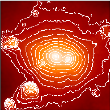
Figure 1: Flux map of the simulated galaxy cluster in the [0.1,10.0] keV energy range binned to $1\arcsec$ pixels. The angular size of the map is 8.3 arcmin, corresponding to approximately 1.7 (proper) Mpc at the cluster redshift $z=0.21$. The superimposed isocontours are obtained from the image after a Gaussian smoothing with $\sigma=8^{\prime\prime}$. Levels are spaced by a factor of $2$ with the highest level corresponding to $1.8\times 10^{-15}$ erg cm^-2 s^-1.

In Fig. 2 we show the photon image of the 300 ks Chandra ACIS-S3 observation of the simulated cluster shown in Fig. 1, as obtained by applying the second unit of our software X-MAS. The image, extracted from the event file in the [0.3,9.0] keV energy band, is background-subtracted, vignetting-corrected, and binned to $1\arcsec$ pixels. We notice that, as expected, after being observed with Chandra, the spatial features present in the simulation, but fainter than the instrument background, are no longer detected. For example, the three faint subclumps on the North, North-West and South-West, clearly visible in Fig. 1, have been washed out in Fig. 2. Conversely all the brighter features appear to be well reproduced by our simulator. We find that this is true even on scales as small as few arcsecs: the previously mentioned angular artifacts of the simulation on these scales are well visible in the photon image, indeed.

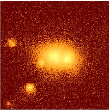
Figure 2: Photon image in the [0.3,9.0] keV energy band of the 300 ks ACIS-S3 observation of the same galaxy cluster shown in Fig. 1. The image is background-subtracted, vignetting-corrected, and binned to $1\arcsec$ pixels.

4 Spectral analysis: preliminary tests

The spectral analysis of Chandra observations of the simulated clusters is done by applying standard procedures and tools used for real observations. In particular, in order to extract spectra, we use the dmextract tool of the CIAO software (see http://cxc.harvard.edu/ciao/). Spectra are extracted in the [0.6,9.0] keV band in PI channels, re-binned to have a minimum of 10 counts per bin and fitted using the XSPEC package (Arnaud 1996). As background we use the spectrum extracted from the publicly available background dataset described in Section 2.2. The position-dependent RMFs and ARFs are computed and weighted by the X-ray brightness over the corresponding image region using the “calcrmf” and “calcarf” tools. Spectra are fitted with a single temperature absorbed mekal model using the C-statistics (Cash 1979; Arnaud 1996) and the Levenberg-Marquardt minimization method (i.e. the XSPEC default minimization method). In the fit procedure we fix the cluster redshift, metallicity, and hydrogen column density to the values used as inputs to compute the Chandra observation. As result of the fit we obtain what, from now on, we call projected spectroscopic temperature and its 68 per cent confidence level error for one interesting parameter, $T_{\rm spec}$ and $\sigma_{\rm spec}$, respectively.

Our goal is to use our Chandra simulator to compare the spectroscopic temperature $T_{\rm spec}$ to one of the possible temperature estimator adopted in the analysis of the results of hydro-N-body simulations. In particular we use the emission-weighted temperature $T_{\rm sim}$, which is the one most commonly adopted. This is defined as:

$$T_{\rm sim}\equiv\frac{\int WTdV}{\int WdV}\ .$$ (3)

In the previous equation, $T$ is the cluster gas temperature, $dV$ is the volume along the line of sight, while the characteristics of the emissivity are taken into account by the weight $W$, which is usually defined as $W=\Lambda(T)\rho^{2}$, where $\Lambda(T)$ is the cooling function and $\rho$ the gas density (see, e.g., Navarro, Frenk & White 1995). The emission-weighted temperature for a specific cluster region is derived directly from the original hydro-N-body simulation by:

$$T_{\rm sim}=\frac{\sum_{i}m_{i}\rho_{i}\Lambda(T_{i})T_{i}}{\sum_{i}m_{i}\rho_{i}\Lambda(T_{i})}\ ,$$ (4)

where the sums are extended to all the particles which are projected inside the considered region. To measure the deviation from a completely isothermal distribution for the gas within the projected region, we use the relative emission-weighted temperature dispersion, defined as

$$\frac{\sigma_{{}_{T}}}{T_{\rm sim}}=\frac{1}{{T_{\rm sim}}}\left[{\frac{\int WT^{2}dV}{\int WdV}-T_{\rm sim}^{2}}\right]^{1/2}\ :$$ (5)

quasi-isothermal and highly perturbed regions will have low and high values of $\sigma_{{}_{T}}/T_{\rm sim}$, respectively.

In the following subsections, we will compare $T_{\rm spec}$ to $T_{\rm sim}$ in two specific cases: i) an ideal toy-model corresponding to a perfect isothermal cluster, and ii) a more realistic cluster with a complex thermal structure.

4.1 Toy isothermal cluster

Here we discuss how the spectroscopically inferred temperature $T_{\rm spec}$ is affected by the total number of detected photons. At this goal we take our simulated cluster and set the temperature of all gas particles to an arbitrarily chosen constant value, $T_{\rm sim}$, ranging from 3 to 12 keV. After producing a 300 ks Chandra observation of this isothermal cluster, we extract all the spectra from each of the $32^{2}$ pixels tile regions, defined in Section 2.2. As the total number of photons in each spectrum is proportional to the total cluster emissivity in the tile region where it was extracted from, this simple procedure allows us to produce a distribution of spectra with the same temperature, but different total photon counts. Among the extracted spectra we select only the ones for which the source flux is higher than the background. For the exposure time and the fixed region size here considered, this is equivalent to selecting spectra with net total counts $N_{\gamma}>250$.

Consistently with what already discussed in literature (see, e.g., Nousek & Shue 1989 and references therein), we find a small bias between the input temperature and the best fit value of the temperature obtained from spectra with small total number counts ($N_{\gamma}<10^{3}$). This bias increases if the total number counts gets smaller and/or the temperature is higher. Nevertheless, we find that the input temperature value is always consistent within the 1$\sigma$ errors associated with the spectroscopic temperature.

4.2 Realistic cluster with a complex thermal structure

To study the effect of temperature inhomogeneities on the final projected temperature estimates we repeat the analysis of the previous subsection using the actual photon temperatures obtained from the simulation, instead of forcing them to be isothermal. As in § 4.1 we selected only spectra for which the source flux is higher than the background (net total counts $N_{\gamma}>250$). We estimate $T_{\rm spec}$ and its error $\sigma_{\rm spec}$ by fitting the data with an absorbed single temperature thermal model.

The result of our analysis is shown in Fig. 3. All the considered spectra are divided in three bins with increasing relative emission-weighted temperature dispersion $\sigma_{{}_{T}}/T_{\rm sim}$ (see equation 5). The three bins, containing the same number of spectra, correspond to regions that, from the point of view of the temperature distribution, are highly homogeneous (i.e. almost isothermal), mildly inhomogeneous and highly inhomogeneous, respectively. For each spectrum we calculate the temperature discrepancy between the spectroscopic and the emission-weighted estimates, $(T_{\rm spec}-T_{\rm sim})/T_{\rm sim}$. The points in the figure represent the median discrepancy in each bin and are located at the median value of $\sigma_{{}_{T}}/T_{\rm sim}$. The vertical error bars represent the 25 and 75 percentiles of the distribution of the discrepancy $(T_{\rm spec}-T_{\rm sim})/T_{\rm sim}$ inside each bin. It is interesting to notice that for regions where the temperature structure is not highly inhomogeneous (i.e. $\sigma_{{}_{T}}/T_{\rm sim}<0.5$), on average we find that $T_{\rm spec}$ and $T_{\rm sim}$ are consistent, although it is still possible to obtain discrepancies of the order of 10-15 per cent. Conversely, for highly inhomogeneous regions (i.e. $\sigma_{{}_{T}}/T_{\rm sim}>0.5$), we find a larger discrepancy between the spectroscopic and the emission-weighted temperatures, with on average $T_{\rm spec}$ systematically lower than $T_{\rm sim}$.

Figure 3: Difference between the spectroscopic and the emission-weighted temperature estimates ($T_{\rm spec}$ and $T_{\rm sim}$, respectively), as a function of the degree of thermal inhomogeneity of the gas, measured by $\sigma_{{}_{T}}/T_{\rm sim}$. The points represent the median value in each bin and are located in the median value of $\sigma_{{}_{T}}/T_{\rm sim}$. Vertical error bars indicate the 25 and 75 percentiles of the corresponding distribution inside each bin; horizontal error bars correspond to the bin size.

Concluding this section, we stress that our results clearly show that, when strong temperature inhomogeneities are present, the spectroscopic and the emission-weighted temperature measurements are likely to be inconsistent with each other. Consequently, much attention must be paid in the theoretical interpretation of observational temperatures. Similar conclusions have been reached by an equivalent analysis of Mathiesen & Evrard (2001) in which they compare the overall spectroscopic and emission-weighted temperatures of a ensemble of 24 simulated clusters of galaxies. Although with a large scatter, they claim that the spectroscopic temperature is 20 per cent lower than the emission-weighted one.

5 Examples of applications

In this section we discuss, as examples, two different applications of our simulation method: the computation of temperature profiles and the production of projected temperature maps of galaxy clusters.

5.1 Temperature profiles

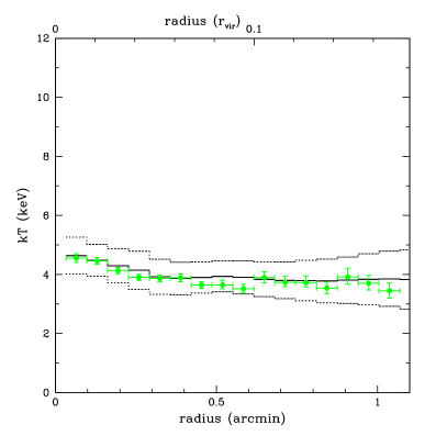
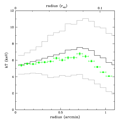
Figure 4: Temperature profiles of the galaxy cluster in two different dynamical phases: a relaxed phase at $z\approx 0.33$ (left panel), and a merging phase at $z\approx 0.21$ (right panel). Dots indicate the temperature profile obtained by fitting the spectra extracted from annular regions centred on the X-ray peak, after the application of our Chandra simulator; error bars are at $68$ per cent confidence level for one interesting parameter. Solid lines refer to the mean emission-weighted temperature directly derived from the simulation, while dotted lines indicate $\sigma_{{}_{T}}$, computed as in equation 5.

One of the standard ingredients of the theoretical modeling of galaxy clusters is the assumption of an isothermal distribution of gas. For example, this is often used to obtain estimates of their mass by using the equation of hydrostatic equilibrium. Another standard application is to directly relate the observed cluster temperature function to the theoretically estimated mass function to obtain constraints on the main cosmological parameters, as the matter density parameter and the normalization and shape of the power spectrum of primordial fluctuations.

However, the results of high-resolution hydro-N-body simulations indicate that the temperature shows radial gradients which cannot be neglected in a dynamical analysis (see, e.g., Evrard, Metzler & Navarro 1996; Eke, Navarro & Frenk 1998; Rasia, Tormen & Moscardini 2003; Borgani et al. 2003). This is confirmed by recent observational data, mainly obtained using the X-ray observatories ASCA, BeppoSAX, and, more recently, Chandra and XMM-Newton (see, e.g., Markevitch et al. 1998; De Grandi & Molendi 2002; Pratt & Arnaud 2002).

In this subsection we use our simulator X-MAS to derive the projected temperature profiles of both a major merging system and a quasi relaxed one. These profiles are compared to the emission-weighted temperature profiles obtained directly from the hydro-N-body simulations. For the merger system we consider the output of the hydro-N-body simulation at redshift $z=0.21$, already described in Section 3 (see Fig. 2). For the relaxed system we use the output of the same simulation at $z\approx 0.33$, when the galaxy cluster is not undergoing any strong merging events. At this redshift the cluster has a virial mass of $3.87\times 10^{14}h^{-1}M_{\odot}$ and a virial radius of $1.7h^{-1}$ Mpc.

To measure the projected temperature profile we extract the spectra from circular annuli centred on the cluster X-ray peak. The size of the bin has been chosen in order to have approximately the same number of photons inside each annulus. Again, spectra are extracted in the [0.3,9.0] keV energy band and fitted with a single temperature absorbed mekal model with the values for $N_{{}_{H}}$, metallicity, and redshift fixed at the simulated values. The spectroscopic temperature profiles $T_{\rm spec}$, together with their relative 68 per cent confidence level errors $\sigma_{\rm spec}$, are shown as filled circles in Fig. 4. Left and right panels refer to the relaxed and merging systems, respectively. In the same figure we show the emission-weighted temperature $T_{\rm sim}$ and the corresponding value of $\sigma_{{}_{T}}$, computed as in equation 5. As discussed in the previous section, the value of $\sigma_{{}_{T}}$ measures the degree of thermal inhomogeneity of the considered cluster region. From Fig. 4 we see that, as expected, the projected radial thermal structure of the cluster in its relaxed phase is far more homogeneous than the structure in the perturbed one. This different degree of thermal homogeneity has strong implications on the temperature profiles. In fact, we notice that while for the relaxed phase the spectral and the emission weighted temperature profiles are in good agreement, this is not longer true for the perturbed phase. Furthermore, we confirm the systematic trend previously discussed: the spectral temperatures are lower than the emission-weighted temperatures.

5.2 Temperature maps

As a further example of possible applications of our X-ray observatory simulation package, we now compare the emission-weighted temperature map determined from the cluster simulation to the projected temperature map obtained from the spectral analysis of its corresponding Chandra observation. In this section we focus only on the output of the hydro-N-body simulation at $z\approx 0.21$, i.e. the perturbed phase considered in Section 3.

First, we calculate the emission-weighted temperature map of the simulated clusters. As the simulation provides us with the density and the temperature of each particle, the emission-weighted temperature map for the simulated cluster can be obtained with the same spatial resolution of its X-ray image. The result is shown in Fig. 5. For reference, in the same figure we superimpose the isocontours corresponding to the cluster flux distribution shown in Fig. 1. As already evident from the temperature profile (see Fig. 4), the internal region is far from being isothermal. Between the two colder central subclumps with $T\approx 5-6$ keV, we notice a region with higher gas temperature, $T\approx 10$ keV, which corresponds to the gas compressed by the merging blobs. Moreover we notice that the more external merging subclumps are also significantly colder than the cluster ambient gas. Of particular interest are the two subclumps on the lower-left corner of the image: they seem to form a single structure of cold gas. In addition, we notice the presence of a shock front with a post-shock gas temperature of approximately 20 keV which is produced by the motion toward the cluster centre of the most internal of these two clumps.

To calculate the spectroscopic projected temperature map we use the 300 ks Chandra observation of the simulated cluster described in Section 3. We extract spectra using adjacent square regions. Over most of the map the extraction regions coincide with the tile regions defined in Section 2.2. However, in the outskirt of the cluster, where the surface brightness is lower, we use larger extraction regions which are obtained by combining two or more tile regions in such a way that the total net number of photons per spectrum is $N_{\gamma}>250$. Each spectrum is then fitted with an absorbed single temperature mekal model with $N_{{}_{H}}$, redshift, metallicity fixed to the input values.

The projected spectroscopic temperature map $T_{\rm spec}$ is shown in the left panel of Fig. 6. In order to make a direct comparison of the spectroscopic temperature map to the emission-weighted one, we degenerate the resolution of the latter to match the former. Thus, in the right panel of Fig. 6 we report the same emission-weighted temperature map shown in Fig. 5, but re-binned as the spectroscopic temperature map of the left panel. It is worth to notice that, although with a lower spatial resolution, the re-binned emission-weighted temperature map presents all the main temperature structures described before. In particular we see that the two central blobs are cold and we can easily identify the compression-heated gas between them. At the same way we can recognize the two cold subclumps on the left-bottom corner, as well as the presence of the shock-heated gas in front of the innermost of the two which is moving toward the cluster centre.

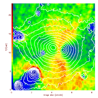
Figure 5: Map of the distribution of the emission-weighted temperature for the galaxy cluster at $z\approx 0.21$ as obtained using the gas particles of the hydro-N-body simulation binned to $1\arcsec$ pixels. The temperature scale (in keV) is shown on the left. The contour levels correspond to the flux distribution shown in Fig. 1.

If we now compare the emission-weighted temperature map on the right to the spectral temperature map on the left, we notice that, although qualitatively similar, they show a number of important differences. Among others, we point our attention on the fact that: i) the central merging blobs appear to be colder in the observed spectroscopic temperature map than in the emission-weighted one; ii) the shock front produced by the motion of the innermost subclump in the lower-left corner, clearly visible in the emission-weighted map, is no longer detected in the spectroscopic temperature map.

To better visualize the temperature differences among the two previous maps, in the left panel of Fig. 7 we show the spatial distribution of the difference $T_{\rm sim}-T_{\rm spec}$. We find temperature differences $|T_{\rm sim}-T_{\rm spec}|>1$ keV for $\ga 50$ per cent of the pixels. In particular we notice that most of these differences are such that $T_{\rm sim}>T_{\rm spec}$. To quantify the significance of this discrepancy, in the right panel of Fig. 7 we present the map of $(T_{\rm sim}-T_{\rm spec})/\sigma_{\rm spec}$ (being $\sigma_{\rm spec}$ the 68 per cent confidence level error associated with the spectroscopic temperature measurement). From this plot we see that most of the temperature differences are significant at $\ga 3\sigma$ confidence level. In particular the temperature discrepancies previously noted for the central subclumps and for the shock regions are significant at $\ga 9\sigma$.

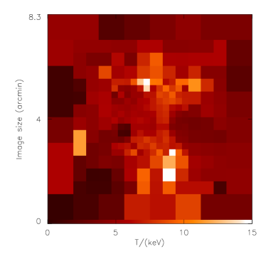
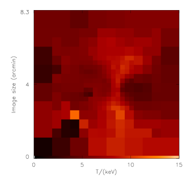
Figure 6: Temperature maps for the galaxy cluster at $z\approx 0.21$. Left panel: map of the projected temperature $T_{\rm spec}$ as derived from the spectroscopic analysis of the Chandra observation. In the outskirt of the cluster, larger regions have been considered in order to have at least 250 net photons per spectrum. Right panel: map of the emission-weighted temperature $T_{\rm sim}$, shown in Fig. 5, but re-binned as in the left panel.

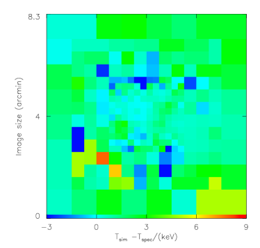
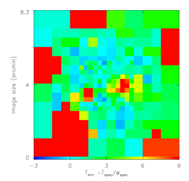
Figure 7: Left panel: map of the differences between the emission-weighted temperature $T_{\rm sim}$ and the spectroscopic projected temperature $T_{\rm spec}$ (right and left panels of Fig. 6, respectively). Right panel: significance level of the temperature differences displayed in the left panel. The map refers to the quantity $(T_{\rm sim}-T_{\rm spec})/\sigma_{\rm spec}$, where $\sigma_{\rm spec}$ is the 68 per cent confidence level error associated with the spectroscopic temperature measurement.

6 Discussion and Conclusions

In this paper we presented a numerical technique and the relative software package X-MAS devoted to simulate X-ray observations of galaxy clusters obtained from hydro-N-body simulations. As specific application, we used this technique to simulate Chandra ACIS-S3 observations.

We stress that one of the main features of our code is that it generates event files following the same standards used for real observations. This is extremely important as it implies that our simulated observations can be analysed in the same way and with the same tools of real observations.

Using the results of high-resolution hydro-N-body simulations, we generated the Chandra observations of a number of simulated clusters. By performing a standard spectral analysis, we derived the projected spectral temperature in specific cluster regions. The spectral temperature has been finally compared to the emission-weighted temperature commonly used to describe to cluster gas thermal properties in numerical works.

Our main finding is that the two temperature estimates are likely to show a significantly large discrepancy, the spectroscopic temperature being lower than the emission-weighted temperature. This effect is more evident if the thermal structure of the cluster within a particular projected region is relatively complex (i.e. the region is thermally highly inhomogeneous). We point out that the data analysis procedure used in this paper assumes that both the background level and spectral shape are well known. In fact the background used to produce the Chandra observations is the same used in the spectral analysis. Uncertainties in the background level and spectral shape, which are quite likely in real observations, would inevitably result in an increase of the estimated errors and in discrepancies between the spectroscopic and emission-weighted temperatures even larger than what has been shown in this paper. Regardless of the background, the main reason behind the observed temperature discrepancy can be easily explained if one considers that spectroscopically the temperature is determined by fitting a thermal model (in particular its bremsstrahlung component) to the observed spectrum. The point is that the sum of two bremsstrahlung spectra with similar emission but different temperatures $T_{1}$ and $T_{2}$ is no longer a bremsstrahlung with a given temperature $T_{3}$. In fact,

$$\exp(-E/T_{1})+\exp(-E/T_{2})\neq A\exp(-E/T_{3})\ ,$$ (6)

unless $T_{1}=T_{2}$. When such a combined spectrum is fitted with a single bremsstrahlung spectral model, we obtain a temperature which is not exactly the mean value of $T_{1}$ and $T_{2}$, though it will be an intermediate value between the two. The larger is the difference $|T_{2}-T_{1}|$, the bigger will be the discrepancy between the spectroscopic and the mean temperature. This result is important because it implies that much attention must be paid in the theoretical interpretation of observational temperatures. Just to give a more detailed idea of the problem, in Section 5 we discussed the implications for two specific cases in which such comparisons have been done in the past: temperature profiles and temperature maps.

Hydro-N-body simulations have been (and still are) largely used to derive universal temperature profiles for galaxy clusters. These profiles are directly compared to the ones obtained from real observations. In Section 5.1 we used the Chandra simulator to compare spectroscopic and emission-weighted temperature profiles of two extreme phases of the cluster evolution: an almost relaxed system and a highly perturbed object. In agreement with what said before, we find that if the cluster is relaxed, the emission-weighted temperature profile agrees with the spectroscopic one. However, if the system is highly perturbed this is not longer true. This result indicate that direct comparisons of observed and “simulated” temperature profiles are not fully justified. In Section 5.2 we show that a similar problem applies also to the temperature maps.

In a forthcoming paper we intend to use X-MAS to investigate in detail a number of problems related to the actual observations of X-ray galaxy clusters. In particular we intend to study the complex problem of spectral deprojection and relative cluster mass determination. Moreover we are planning to use X-MAS to perform observations of simulated clusters that account for the processes of the metal enrichment of the ICM. This will allow us to address the even more complex problem of determining both the mean and the single-element metallicity structure of real galaxy clusters.

To conclude we stress that the possible applications of our simulations of observations are quite vast. Besides the here discussed problem of the comparisons of outputs of numerical simulations to real observed galaxy clusters, it can be very useful to better plan observations with existing X-ray telescopes and even more to verify what will be the real capabilities of futures ones. At this goal, results obtained by using X-MAS will be soon publicly available on the web.

Concerning our software package, we remind that at present we only completed the software module that simulates ACIS-S3 Chandra observations. Work is in progress to include further modules to simulate Chandra observations in the ACIS-I mode, and XMM-Newton observations with both EPIC and MOS detectors.

References

- [1] Arnaud K.A., 1996, ASP Conf. Ser. 101, Astronomical Data Analysis Software and Systems V, G.H. Jacoby & J. Barnes eds., 5, 17
- [2] Blanton E.L., Sarazin C.L., McNamara B.R., Wise M.W., 2001, ApJ, 558, L15
- [3] Borgani S., et al., 2003, preprint, submitted to MNRAS
- [4] Cash W., 1979, ApJ, 228, 939
- [5] Churazov E., Forman W., Jones C., Boehringer H., 2003, ApJ, 590, 225
- [6] De Grandi S., Molendi S., 2002, ApJ, 567, 163
- [7] Dolag K., Bartelmann M., Lesch H., 2002, A&A, 387, 383
- [8] Dorman B., Arnaud K.A., 2001, ASP Conf. Ser. 238, Astronomical Data Analysis Software and Systems X. F.R. Harnden Jr., F.A. Primini & H.E. Payne eds. San Francisco: Astronomical Society of the Pacific, p.415
- [9] Eke V.R., Navarro J.F., Frenk C.S., 1998, ApJ, 503, 569
- [10] Evrard A.E., Metzler C.R., Navarro J.F., 1996, ApJ, 469, 494
- [11] Fabian A.C., Sanders J.S., Ettori S., Taylor G.B., Allen S.W., Crawford C.S., Iwasawa K., Johnstone R.M., 2001, MNRAS, 321, L33
- [12] Fabian A.C., et al., 2000, MNRAS, 318, L65
- [13] Heinz S., Choi Y.-Y., Reynolds C.S., Begelman M.C., 2002, ApJ, 569, L79
- [14] Johnstone R.M., Allen S.W., Fabian A.C., Sanders J.S., 2002, MNRAS, 336, 299
- [15] Kaastra J.S., Mewe R., 1993, Legacy, 3, 16
- [16] Kay S.T., Thomas P.A., Theuns T., 2003, MNRAS, 343, 608
- [17] Lewis G.F., Babul A., Katz N., Quinn T., Hernquist L., Weinberg D.H., 2000, ApJ, 623, 644
- [18] Liedahl D.A., Osterheld A.L., Goldstein W.H., 1995, ApJ, 438, L115
- [19] Markevitch M., Forman W.R., Sarazin C.L., Vikhlinin A., 1998, ApJ, 503, 77
- [20] Markevitch M., Vikhlinin A., Mazzotta P., 2001, ApJ, 562, L153
- [21] Markevitch M., et al., 2000, ApJ, 541, 542
- [22] Marri S., White S.D.M., 2003, MNRAS, 345, 561
- [23] Mathiesen B.F., Evrard A.E., 2001, ApJ, 546, 100
- [24] Mazzotta P., Edge A., Markevitch M., 2003, ApJ, 596, 190
- [25] Mazzotta P., Fusco-Femiano R., Vikhlinin A., 2002a, ApJ, 569, L31
- [26] Mazzotta P., Kaastra J.S., Paerels F.B., Ferrigno C., Colafrancesco S., Mewe R., Forman W.R., 2002b, ApJ, 567, L37
- [27] Mazzotta P., Markevitch M., Vikhlinin A., Forman W.R., David L.P., VanSpeybroech L., 2001, ApJ, 555, 205
- [28] McNamara B.R., et al., 2000, ApJ, 534, L135
- [29] McNamara B.R., et al., 2001, ApJ, 562, L149
- [30] Morrison R., McCammon D., 1983, ApJ, 270, 119
- [] Muanwong O., Thomas P.A., Kay S.T., Pearce F.R., 2002, MNRAS, 336, 527
- [31] Navarro J.F., Frenk C.S., White S.D.M., 1995, MNRAS, 275, 720
- [32] Nousek J.A., Shue D.R., 1989, ApJ, 342, 1207
- [33] Pratt G.W., Arnaud M., 2002, A&A, 394, 375
- [34] Rasia E., Tormen G., Moscardini L., 2003, preprint, astro-ph/0309405
- [35] Sanders J.S., Fabian A.C., 2002, MNRAS, 331, 273
- [36] Schindler S., Castillo-Morales A., De Filippis E., Schwope A., Wambsganss J., 2001, A&A, 376, L27
- [37] Schmidt R.W., Fabian A.C., Sanders J.S., 2002, MNRAS, 337, 71
- [38] Smith D.A., Wilson A.S., Arnaud K.A., Terashima Y., Young A.J., 2002, ApJ, 565, 195
- [39] Springel V., Hernquist L., 2003, MNRAS, 339, 289
- [40] Springel V., Yoshida N., White S.D.M., 2001, NewA, 6, 79
- [41] Tormen G., Bouchet F.R., White S.D.M., 1997, MNRAS, 286, 865
- [42] Tormen G., Moscardini L., Yoshida N., 2003, preprint, astro-ph/0304375
- [43] Tornatore L., Borgani S., Springel V., Matteucci F., Menci N., Murante G., 2003, MNRAS, 342, 1025
- [44] Vikhlinin A., Markevitch M., Murray S.S., 2001, ApJ, 551, 160
- [45] Yoshida N., Stoehr F., Springel V., White S.D.M., 2002, MNRAS, 335, 762
- [46] Young A.J., Wilson A.S., Mundell C.G., 2002, ApJ, 579, 560