The Effect of Proton Temperature Anisotropy on the Solar Minimum Corona and Wind
Abstract
A semi-empirical, axisymmetric model of the solar minimum corona is developed by solving the equations for conservation of mass and momentum with prescribed anisotropic temperature distributions. In the high-latitude regions, the proton temperature anisotropy is strong and the associated mirror force plays an important role in driving the fast solar wind; the critical point where the outflow velocity equals the parallel sound speed () is reached already at 1.5 from Sun center. The slow wind arises from a region with open field lines and weak anisotropy surrounding the equatorial streamer belt. The model parameters were chosen to reproduce the observed latitudinal extent of the equatorial streamer in the corona and at large distance from the Sun. We find that the magnetic cusp of the closed-field streamer core lies at about 1.95 . The transition from fast to slow wind is due to a decrease in temperature anisotropy combined with the non-monotonic behavior of the non-radial expansion factor in flow tubes that pass near the streamer cusp. In the slow wind, the plasma is of order unity and the critical point lies at about 5 , well beyond the magnetic cusp. The predicted outflow velocities are consistent with Doppler dimming measurements from UVCS/SOHO. We also find good agreement with polarized brightness () measurements from LASCO/SOHO and H I Ly images from UVCS/SOHO.
1 Introduction
At the time of cycle minimum, the solar corona is more or less axisymmetric and stable for many months. The polar coronal holes are separated by an equatorial streamer belt that encircles the Sun. The fast solar wind originates from the coronal holes, while the slow wind originates from the vicinity of the streamer belt. The physical processes that drive the fast and slow wind are only partially understood. In particular, it is unclear why the Sun has such a bimodal outflow pattern with distinctly different physical conditions in the fast and slow wind. Does this distinction between fast and slow wind already exist at low heights in the corona, or does it arise only at larger distance from the Sun? What causes the transition from fast to slow wind as we approach the solar equator? What is the role of open and closed magnetic fields in this transition? To answer such questions, an empirical description of the corona is needed; i.e., a description of temperature, density, velocity and magnetic field as function of latitude, longitude and radial distance from the Sun. Such modeling is a necessary step in the study of the physical processes by which the fast and slow wind are generated.
Axisymmetric, semi-empirical models of the solar corona have been developed by many authors (e.g., Pneuman & Kopp, 1971; Yeh & Pneuman, 1977; Steinolfson, Suess & Wu, 1982; Washimi, Yoshino & Ogino, 1987; Cuperman et al., 1990, 1993; Wang A. H. et al., 1993, 1998a; Lionello, Linker & Mikic, 2001). For example, Sittler & Guhathakurta (1999) used empirically derived electron density profiles to construct a model of the magnetic field, outflow velocity, effective temperature, and effective heat flux. These parameters are derived by solving the equations for conservation of mass, momentum and energy, and the magnetic induction equation. The model provides an estimate of the large-scale surface magnetic field at the Sun, which is estimated to be 12-15 G. The authors predict that the large-scale surface field is dominated by an octupole term. More recently, three-dimensional models of the corona have also been developed (e.g., Linker, Van Hoven & Schnack, 1990; Wang Y.-M. et al., 1997a; Riley, Linker & Mikic, 2001).
In this paper we develop a coronal model that synthesizes observational data obtained with instruments on the Solar and Heliospheric Observatory (SOHO) satellite, in particular data from the Ultraviolet Coronagraph Spectrometer (UVCS; Kohl et al., 1995). UVCS observations have shown that the minor ions in coronal holes have kinetic temperatures that are much larger than those for protons and electrons (Kohl et al., 1998; Cranmer et al., 1999). Here kinetic temperature refers to the total velocity dispersion of the particles, including thermal and non-thermal components. Detailed analysis of kinetic temperatures for different ions has shown that some ions have higher temperature than others, indicating preferential heating of certain ions. Furthermore, Doppler dimming analysis of spectral lines such as O VI 1032 and 1037 has shown that some minor ions have anisotropic velocity distributions: the velocity dispersion perpendicular to the (nearly radial) magnetic field in coronal holes is significantly larger than that parallel to the field. This high temperature and large temperature anisotropy of the ions is believed to be caused by dissipation of transverse waves (Dusenbery & Hollweg, 1981; Isenberg & Hollweg, 1983; Tu & Marsch, 1997; Cranmer et al., 1999; Hu & Habbal, 1999). A similar but smaller anisotropy may also exist for the protons (Cranmer et al., 1999). In the presence of a diverging magnetic field, charged particles experience an outward force that causes the perpendicular motion of the particles to be converted into parallel motion. Therefore, if the perpendicular energy of the protons is continually replenished by wave dissipation, the protons can maintain an anisotropic velocity distribution () and there is a net outward force on the protons. This so-called mirror force plays an important role in driving the fast solar wind (see review by Cranmer, 2002).
The purpose of the present paper is to include the effects of proton temperature anisotropy into a global model of the solar corona. The paper is organized as follows. In §2 we discuss observations of streamers and the relationship between the streamer and the slow solar wind. In §3 we present observational constraints on our global model, including temperature and density in the corona and magnetic flux at the coronal base. In §4 we present a method for solving the coronal force balance equations, taking into account the mirror force. In §5 we present our model results for coronal magnetic structure and outflow velocity. In §6 we derive images of visible light polarization brightness and H I Ly intensities from our model, and we compare our results with observations. The main results of this work are discussed in §7.
2 Streamer Structure and the Origin of the Slow Wind
The K corona is produced by Thomson scattering of photospheric white light by free electrons in the corona. In a study of the solar minimum corona using the Large Angle and Spectrometric Coronagraph (LASCO) on SOHO, Wang Y.-M. et al. (1997a) found that the large-scale structure of the coronal streamer belt at 3 and beyond can be reproduced with a model in which the scattering electrons are concentrated around a single, warped current sheet that encircles the Sun. The angular width of this sheet is only a few degrees. The bright, narrow spikes seen in LASCO C2 and C3 images occur wherever the sheet is oriented edge-on in the plane of the sky (Wang Y.-M. et al., 1998b). In contrast, the latitudinal extent of the slow wind, as determined from in-situ measurements, is about (Suess et al., 1999), much larger than the thickness of the coronal plasma sheet observed with LASCO. This implies that the bulk of the slow wind originates from open field lines outside the observed plasma sheet (Wang Y.-M. et al., 1998b).
Sheeley et al. (1997) used time-lapse sequences of LASCO images to track the outward motion of small density enhancements (“blobs”) in the plasma sheet. These blobs originate in the high corona above the top of the helmet streamer, and slowly accelerate outward though the LASCO field of view (2.2-30 ). Wang Y.-M. et al. (1998b) suggest that both the blobs and the plasma sheet represent closed-field material injected into the slow wind as a result of foot-point exchanges between the stretched helmet-streamer loops and neighboring open field lines. According to this model, the ejection of the blobs does not cause any permanent disruption of the helmet streamer, which remains in a stretched, quasi-equilibrium state with its cusp at 3 .
Noci et al. (1997) and Raymond et al. (1997) observed the equatorial streamer with UVCS/SOHO at radii between 1.5 and 5 . Images of the streamer in O VI 1032 show two bright legs separated by a dark lane. This lane extends radially along the streamer axis up to 3 (also see Strachan et al., 2002; Frazin, Cranmer & Kohl, 2003). In contrast, H I Ly and white-light images do not show such a dark feature. This led Noci et al. (1997) to attribute the dark lane to a reduced oxygen abundance along the streamer axis. Raymond et al. (1997) further suggested that this abundance anomaly is due to gravitational settling of oxygen in the static proton/electron plasma of the closed-field streamer core. If this interpretation is correct, the closed field lines must extend up to 3 , consistent with the model of Wang Y.-M. et al. (1998b).
The O VI images for July 1996 show that the streamer legs converge towards the equator in the range 2-2.5 from Sun center. This suggests that the streamer cusp may be located at about 2 , somewhat less than implied by the model of Wang Y.-M. et al. (1998b). We propose the following scenario. The blobs observed by Sheeley et al. (1997) originate at the cusp (2 ), but become clearly visible only at somewhat larger height (3-4 ). The plasma within the blobs originates in the closed-field streamer core, which is affected by gravitational settling. Therefore, the blobs have low oxygen abundance compared to the surrounding slow solar wind. As the blobs move out into the region between 2 and 3 , they contribute to reduced O VI emission along the axis of the streamer. In this way, the effects of gravitational settling are transmitted to larger height via the blobs. In contrast, the open field lines farther away from the streamer axis always have a slow outflow and therefore are unaffected by settling.
Strachan et al. (2002) measured outflow velocities in streamers using the Doppler dimming effect (also see Habbal et al., 1997). In a latitudinal scan at 2.33 , Strachan et al. found no measurable outflow velocity within the streamer ( km/s), but a steep rise in outflow velocity occurs just beyond the bright streamer legs. The latitudinal width of the streamer, as defined by the point where the outflow velocity equals 100 km/s, is about (see Fig. 4d of Strachan et al., 2002), similar to the observed width of the slow wind at large distance from the Sun (Suess et al., 1999).
3 Observational Constraints on Global Model
This section describes the observational constraints on coronal density, temperature, and magnetic flux to be used in §4.
3.1 Electron Density
The polarized brightness () of the K corona can be used to measure the coronal electron density (van de Hulst, 1950). Here we use the results of Guhathakurta, Holzer & MacQueen (1996) and Sittler & Guhathakurta (1999), who used Skylab data from 1973-1974 to derive electron density profiles for coronal holes and streamers at cycle minimum (see also Newkirk, 1967; Allen, 1973; Munro & Jackson, 1977; Saito et al., 1977). Their results are expressed in terms of radial profiles, one for the polar coronal hole, another for the equatorial streamer. They used the following expression for the electron density within each component:
| (1) |
where is the heliocentric distance in units of , and the parameters are given by Sittler & Guhathakurta (1999). The density profiles are shown in Figure The Effect of Proton Temperature Anisotropy on the Solar Minimum Corona and Wind. The Skylab data span the height range and were further extrapolated using data from the Ulysses mission (Phillips et al., 1995). These measurements correspond to select days when the equatorial streamer belt was seen approximately end-on. This explains why their streamer densities are somewhat larger than those of Saito et al. (1977), who presented streamer densities averaged over many days.
3.2 Electron Temperature
One method for inferring the electron temperature is to use spectral line intensity ratios of two lines from the same ion. Wilhelm et al. (1998) used data from SUMER/SOHO to estimate at radii 1.03-1.6 in coronal holes at the last cycle minimum (1996-1997). They use Mg IX 706 Å and 750 Å, and they conclude that in both the plume and inter-plume regions the electrons barely reach the canonical temperature of 1 MK. Moreover, falls off rapidly with height. Although their temperature estimates depend on atomic data that, according to the authors, could be improved, their work suggests that in polar hole regions the electrons are significantly cooler than the ions (see Landi et al., 2001, for a quantitative analysis on uncertainties of estimates, derived from Be-like line ratios and using different theoretical methods).
The rates of ionization and recombination of coronal ions decrease rapidly with distance from the Sun. Therefore, the charge state of the solar wind is determined in large part by the electron temperature in the inner corona where the ionization and recombination times are still short compared to the solar wind expansion time. In situ measurements of the solar wind charge state can be used to estimate the coronal electron temperature. Ko et al. (1997) derived polar profiles from observations with SWICS/Ulysses. Their results can be approximated as a combination of two power laws (see Cranmer et al., 1999):
| (2) |
Raymond et al. (1997) and Li et al. (1998) studied the ionization balance of various ions in a streamer observed with UVCS/SOHO in July 1996. The results indicate that reaches a maximum value of about 1.6 MK in the streamer core. Due to the high density and low outflow velocity in streamers (e.g., Frazin, 2002), we expect that protons and electrons are in thermal equilibrium with each other, so the electrons may be used as a proxy for the protons. Raymond et al. (1997) and Li et al. (1998) show that their observations are compatible with hydrostatic equilibrium in the streamer core (Gibson et al., 1999, also see). In this paper we derive the electron temperature from the observed electron density , assuming hydrostatic equilibrium.
In this paper we use a generalization of expression (2) to describe the radial variation of electron temperature at the pole and the equator:
| (3) |
where is the temperature at the coronal base (). The values of the parameters , , and are given in Table 1, and the profiles are shown in Figure The Effect of Proton Temperature Anisotropy on the Solar Minimum Corona and Wind. The electron temperature model at the poles (dashed line) has been adjusted to approximately fit the observational data of Ko et al. (1997) and Cranmer et al. (1999) (triangles). The electrons are assumed to have a Maxwellian velocity distribution. The electron temperature at the equator (thick line) is assumed to be equal to the proton temperature, discussed in the next section.
3.3 Proton Temperature
Ion temperatures can be estimated by measuring the width of coronal emission line profiles. Due to rapid charge exchange between protons and neutral hydrogen, the latter can be used as a proxy for the protons. Allen, Habbal & Hu (1998) studied the coupling between neutral hydrogen and protons by treating the hydrogen atoms as test particles in a proton-electron background. Their work indicates that the H I velocity distribution reflects the proton distribution at radii up to about 3 in the polar regions and even higher in the equatorial regions. Above 3 in the polar regions, the H I velocity distribution “follows” the proton distribution and reaches temperatures about 20% higher than the protons (see also Olsen, Leer & Holzer, 1994; Olsen & Leer, 1996). These results strongly support the use of H I Ly profiles to measure the velocity spread of the protons along the line of sight (LOS). The observed velocity spread includes both thermal and non-thermal components (such as wave motions), and may also include a contribution from solar wind expansion in the direction along the LOS (most emission originates near the point of closest approach to the Sun, but there is some contribution from regions behind and in front of the plane of the sky where the solar wind velocity has a component along the LOS). Therefore, the velocity spread derived from the observed line width provides only an upper limit on the proton temperature: , where is the observed velocity spread, is the hydrogen mass and is Boltzmann’s constant. At the time of cycle minimum, the polar coronal holes are very large, and polar observations at are unaffected by low-latitude streamers.
UVCS/SOHO observations of heavier ions such as show that the velocity distributions of these ions in coronal holes are highly anisotropic: the velocity spread in the radial direction (as derived from Doppler dimming analysis) is much smaller than that in the tangential direction (Kohl et al., 1998; Cranmer et al., 1999). It is unclear whether this anisotropy also exists for the protons; Doppler dimming analysis of H I Lyman lines does not provide strong constraints on the proton parallel velocity in coronal holes. The anisotropy is believed to be due to the damping of transverse waves (e.g., due to ion-cyclotron resonance), and this perpendicular heating may also occur for the protons. In this paper we assume that the protons indeed have an anisotropic velocity distribution in the low-density polar regions (), but not in the equatorial region (). Since the magnetic field over the pole is approximately radial and perpendicular to the LOS, the observed H I Ly line width provides an estimate for the proton perpendicular temperature. Furthermore, we assume that the proton parallel temperature equals the (isotropic) electron temperature, , so that the radial variation of at the pole and equator is given by equation (3) with parameter values given in Table 1. The anisotropy in proton temperature over the pole is consistent with in-situ measurements, which show that in the solar wind (Marsh et al., 1982; Pilipp et al., 1987).
Kohl et al. (1998) and Cranmer et al. (1999) analyzed H I Ly line profiles observed in polar coronal holes during the past cycle minimum (1996-1997). Their results indicate proton perpendicular temperatures up to 6 MK. The observed velocity width () increases rapidly with height from about 190 km/s ( MK) at 1.5 , to 240 km/s ( MK) at 2.5 , and then slowly decreases to 250 km/s ( MK) at 4 . The results are consistent with earlier measurements from UVCS/Spartan by Kohl, Strachan & Gardner (1996), who found peak temperatures of 5-6 MK at 2.25 and 3.5 MK at 3.5 in a polar coronal hole in 1993. From these several observations, measured temperatures at different heights are shown by asterisks in Figure The Effect of Proton Temperature Anisotropy on the Solar Minimum Corona and Wind.
UVCS/SOHO observations in the equatorial regions indicate a roughly constant proton temperature within the core of the streamer belt. We reanalyzed UVCS data from a super-synoptic campaign during July 1996 (Raymond et al., 1997), and find Ly line widths of order 185 km/s ( MK) at 1.5 and 195 km/s ( MK) at 2.6 . At larger heights, the line widths decrease to 170 km/s ( MK) at 3 and 150 km/s ( MK) at 4.5 . The measurements are shown by the crosses in Figure The Effect of Proton Temperature Anisotropy on the Solar Minimum Corona and Wind. Streamer observations by Kohl et al. (1997), obtained about a month after the Raymond observations, exhibit very similar values (2.2 MK at 2 , 1.5 MK at 4 ).
In this paper we use the following expression for the proton perpendicular temperature:
| (4) |
The first term is similar to that used for the electron temperature, but the second term allows us to impose a further increase in temperature over a limited range of heights (of order ), consistent with UVCS observations. The values of the parameters at the pole and at the equator are given in Table 1.
In summary, our temperature models present the following main features: (1) at the pole, strong anisotropy for protons, and electron temperature much lower than ; (2) at the equator, hydrostatic equilibrium isotropic velocity distributions and thermal equilibrium between species. Note that and are the same for all temperature models, so that at low heights in the corona.
3.4 Magnetic Flux at Coronal Base
Figure The Effect of Proton Temperature Anisotropy on the Solar Minimum Corona and Wind shows the longitude-averaged radial magnetic field as function of latitude at the solar surface (). These data are derived from the Kitt Peak synoptic map for July 1996, near the time of cycle minimum. There are no large active regions on the Sun at this time. The full curve in Fig. The Effect of Proton Temperature Anisotropy on the Solar Minimum Corona and Wind is a fit of the form
| (5) |
where and = +10 G. Note that decreases monotonically from about +10 G in the North to -10 G in the South. At latitudes between degrees, the average radial field is very small (less than 2 G). Therefore, the large-scale coronal field is dominated by the polar fields.
4 Coronal Model with Anisotropic Gas Pressure
At cycle minimum, the corona presents a relatively ordered structure with high latitude coronal holes and an equatorial streamer belt. The corona is essentially axisymmetric and stable for many months (e.g., Gibson, 2001). In the following we describe an axisymmetric model of the corona; an earlier version of this model was described by Vásquez, Raymond & van Ballegooijen (1999) and Vásquez, van Ballegooijen & Raymond (1999). We use a spherical coordinate system and assume that all scalar quantities are independent of azimuth . The magnetic field is assumed to lie in the meridional plane:
| (6) |
where is the vector potential, and is the field-line variable (note that = constant along field lines). This variable increases from along the polar axis to at the equator (, ). There is a critical field line that forms the boundary between open and closed magnetic regions; the field lines with are open, while those with are closed. Note that is the fraction of surface flux that is open. In this paper we assume = 0.80. The magnetic configuration is illustrated in Figure The Effect of Proton Temperature Anisotropy on the Solar Minimum Corona and Wind.
Rather than solving an energy equation for the coronal plasma, our semi-empirical model is based on observed temperature distributions. The electron and proton temperatures (, and ) are interpolated between the pole and equator:
| (7) |
where and are the observed profiles described in §3, and is a function of the field-line variable that increases monotonically from at the pole to at the equator. We use the following expression for :
| (8) |
where is the mid-point of the transition [], and measures the width of the transition. In this paper we use = 0.70 and = 0.15. The function is shown in Figure The Effect of Proton Temperature Anisotropy on the Solar Minimum Corona and Wind.
The coronal magnetic and velocity fields are computed by solving the momentum equation:
| (9) |
where is the pressure tensor, is the mass density, is the outflow velocity, is the gravitational potential. The steady-flow condition requires that , and conservation of mass requires that is constant along field lines. The pressure tensor is anisotropic:
| (10) |
where is the unit tensor, is the unit vector along , and and are the parallel and perpendicular pressures:
| (11) | |||||
| (12) |
Here we assume a pure hydrogen plasma. The left-hand side of equation (9) can be written as
| (13) |
where measures distance along the field lines, , , and we used . The component of the momentum equation (9) parallel to reads
| (14) |
and the solution of this equation will be further discussed in §4.2. We now introduce the function describing the dependence of on the field-line variable: . Then the gradient of is
| (15) |
where the partial derivatives on the RHS are taken at constant and constant , respectively. It follows that , where is the angle between and , and similarly . Inserting these expressions into equation (14), we obtain
| (16) |
and combining equation (9), (13), (15) and (16) yields
| (17) |
In streamers the pressure anisotropy and outflow velocity are small, so the terms involving can be neglected. The same is true in coronal holes because in these regions the magnetic field is nearly radial and the vectors and vanish for radial fields. Therefore, plays only a minor role in the perpendicular force balance, and we will neglect its effects in equation (17). Then the perpendicular force balance (17) reduces to
| (18) |
where we used equation (6). The solution of equation (18) will be discussed in §4.1.
We use an iterative method for solving equations (16) and (18). The method can be summarized as follows. We first construct a preliminary pressure model by interpolating the observed perpendicular pressure between pole and equator, using an expression similar to equation (7). Then we compute the field-line variable by solving the perpendicular force balance as described below in §4.1; this gives us a first guess for the shape of the magnetic field lines. Then we solve the parallel force balance separately along many field lines as described in §4.2. This yields the mass density and velocity along each field line, which are then remapped to produce the density and velocity . We also update the perpendicular pressure , which is then used in the next iteration to recompute the field-line variable . This process is repeated until convergence is achieved. Note that in the first iteration is specified analytically, whereas in subsequent iterations is obtained by numerical interpolation.
4.1 Perpendicular force balance
To solve equation (18) for the perpendicular force balance, we introduce the following integral over the coronal volume:
| (19) |
where only one hemisphere of the Sun is considered, and = 10 is the outer radius of the computational domain. The magnetic field is related to via equation (6), and . At each step in our iterative procedure, is a known function, so depends only on the unknown function , or equivalently, . We assume the following boundary conditions for :
| (20) | |||||
| (21) | |||||
| (22) | |||||
| (23) | |||||
| (24) |
Equation (20) is derived from the surface flux distribution, equation (5), and the magnetic field is assumed to be radial at the outer boundary, . Equations (23) and (24) describe the boundary conditions at the equator. For , there is a current sheet at the equator separating the open fields from the two hemispheres, hence the magnetic field just above the equator is radial. For the magnetic field is closed over the equator, so the field is perpendicular to the equatorial plane.
We now show that the function for which reaches its minimum value is a solution of equation (18). Let be an arbitrary variation of , then the corresponding change in is
| (25) |
where the boundary conditions (20) - (24) have been used. At the minimum, vanishes for any function , so the quantity in square brackets in equation (25) must vanish. This is precisely the condition for perpendicular force balance, equation (18).
The function is discretized on a non-uniform grid in and with 180 points in each direction. The minimization of is performed using the Polak-Ribiere version of the conjugate gradient method (Press, et al., 1992). This is an iterative method for adjusting the values of at the grid points until the minimum of is reached. The cusp radius is also allowed to change in order to obtain the lowest possible , but the amount of open magnetic flux () is held fixed.
4.2 Parallel force balance
The parallel component of the momentum equation (14) can be written in the following form:
| (26) |
where and are the parallel and perpendicular sound speeds:
| (27) |
Using = constant along field lines, we can eliminate the density from equation (26):
| (28) |
where
| (29) |
At each step of our iterative procedure we have estimates for , , , and on any open field line, which allows us to compute the function . According to equation (28), the sonic point () is located at an extremum of . The velocity is found by inward and outward integration of equation (28), starting at the sonic point. In practice we find that, in order to obtain a valid solution over the entire height range (), the sonic point must be located at the global minimum of . The density is computed from mass flux conservation and the boundary condition for the density at the coronal base (see §3). This process is repeated for 180 different open field lines, and the results are remapped to obtain the density and velocity on the grid.
5 Results
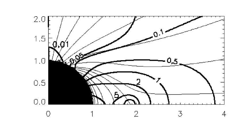
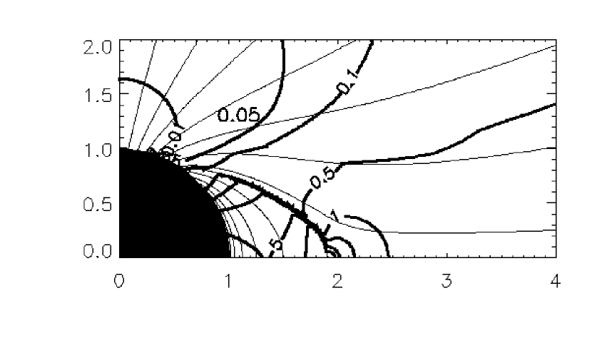
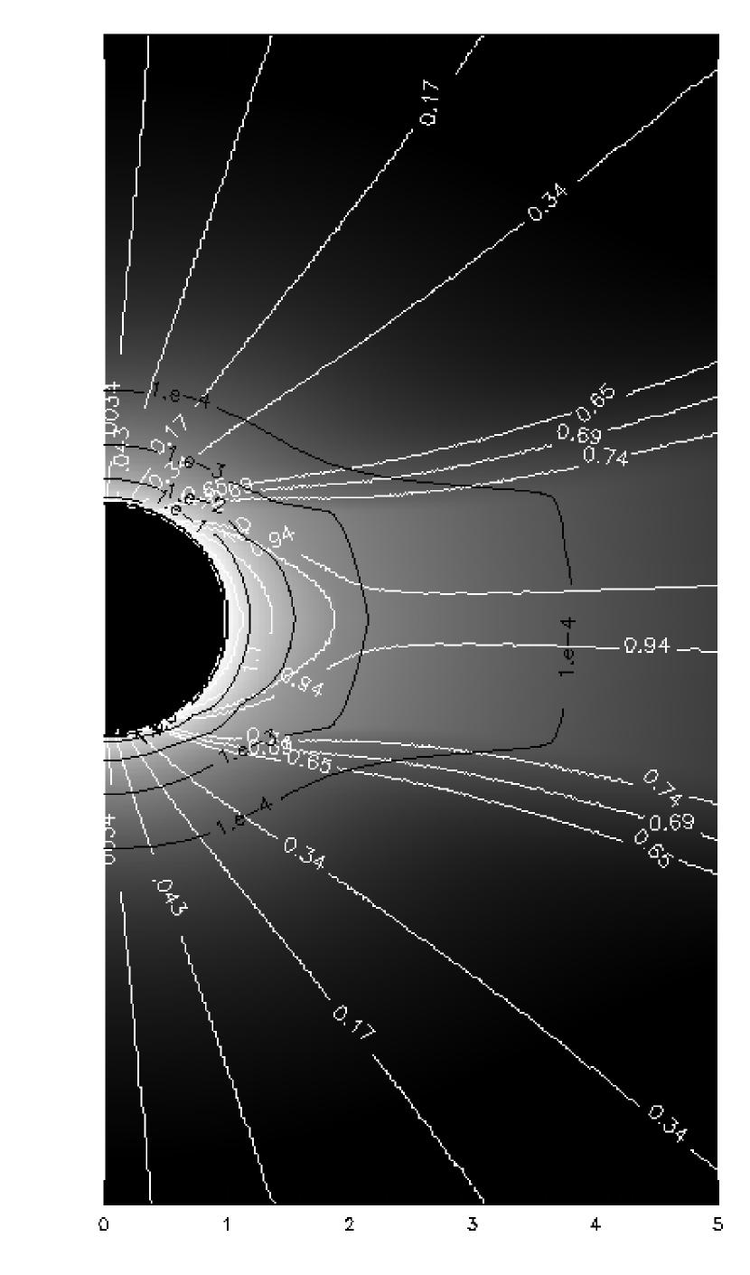
We iterated the parallel and perpendicular force balance equations as described in §4. The process was repeated until the maximum change in between iterations is less than ; this required 20 iterations. The results for the first and last iterations are shown in Figures The Effect of Proton Temperature Anisotropy on the Solar Minimum Corona and Winda and The Effect of Proton Temperature Anisotropy on the Solar Minimum Corona and Windb, respectively. The thin curves represent magnetic field lines, and the thick curves are contours of , the ratio of perpendicular gas pressure and magnetic pressure . The cusp height in the final solution is . Note that the magnetic structure changes little between the first and last iterations.
Our model yields in the polar regions, but in the equatorial streamer, especially near the streamer cusp. This supports the idea that the streamer is magnetically contained by the strong polar fields that surround it on either side (Suess, Gary & Nerney, 1999). We find that throughout the closed-field region of the streamer. However, the variation with height is not monotonic: has peaks at both the cusp and the streamer base, and lower values at intermediate heights. Our results are similar to those of Li et al. (1998), who estimated based on UVCS/SOHO and SXT/Yohkoh observations of streamers (July 1996) in combination with potential field extrapolation of the photospheric magnetic field. Their estimates indicate at 1.15 and at 1.50 , similar to the values found here. High values of were also found in MHD models that include heat and momentum deposition in the corona (Wang A. H. et al., 1998a; Suess et al., 1996).
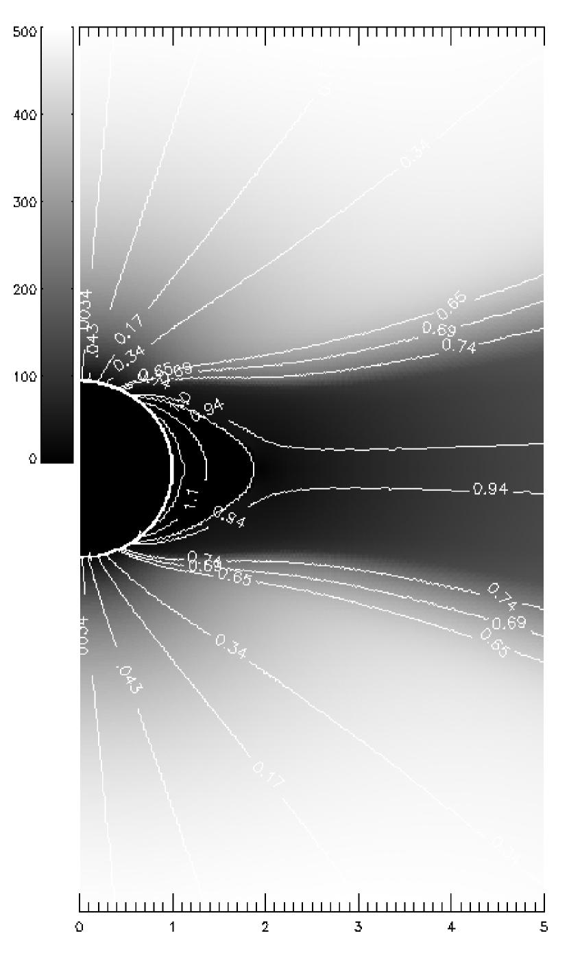
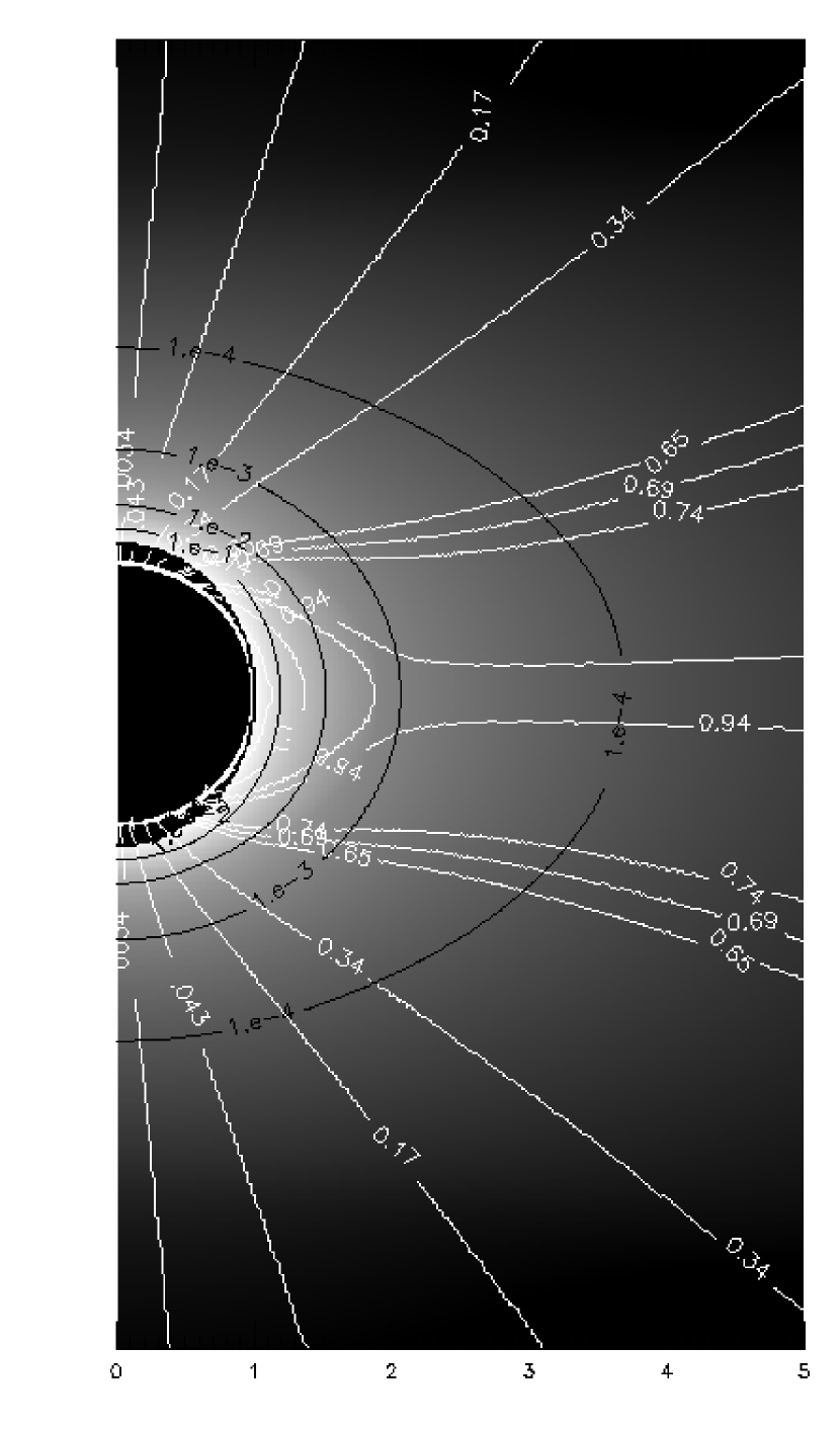
Figure The Effect of Proton Temperature Anisotropy on the Solar Minimum Corona and Wind shows the outflow velocity for the final model. The bright region is the fast solar wind emanating from the coronal hole, and the dark region is the slow wind that flows along the open field lines within the streamer. The maximum velocities are about 450 km/s for the fast wind and 190 km/s for the slow wind. This is somewhat smaller than the observed in-situ values at 1 AU (800 and 400 km/s, respectively). We attribute this difference to the fact that our model does not include any momentum deposition effects other than the mirror force. However, the ratio of fast and slow wind speeds is about 2.5 in our model, consistent with in-situ measurements.
Figure The Effect of Proton Temperature Anisotropy on the Solar Minimum Corona and Wind shows three quantities measured across magnetic field lines: the temperature anisotropy at 3 , the radial position of the sonic point, and the asymptotic wind speed. Note that the variation of wind speed closely follows that of the temperature anisotropy (compare top and bottom panels). This indicates that the fast wind is driven by the high perpendicular temperatures in the coronal hole, and the decrease in wind speed at the edge of the hole is mainly due to the decrease in temperature anisotropy. The middle panel shows that there is a sudden jump in sonic-point radius once the transition from high to low temperature anisotropy is nearly complete. The jump occurs at and is due to the appearance of a second (lower) minimum in the function at a height well beyond the streamer cusp (see below). As a result, the sonic-point radius changes discontinuously from about 1.5 in the coronal hole to about 5.5 in the streamer. Such large values for the sonic-point height in the streamer were found earlier by Wang Y.-M. (1994) and Chen & Hu (2001). Most of the decrease in wind speed occurs for between 0.6 and 0.77, well before the jump in sonic-point height, and the asymptotic wind speed does not change significantly at the jump.
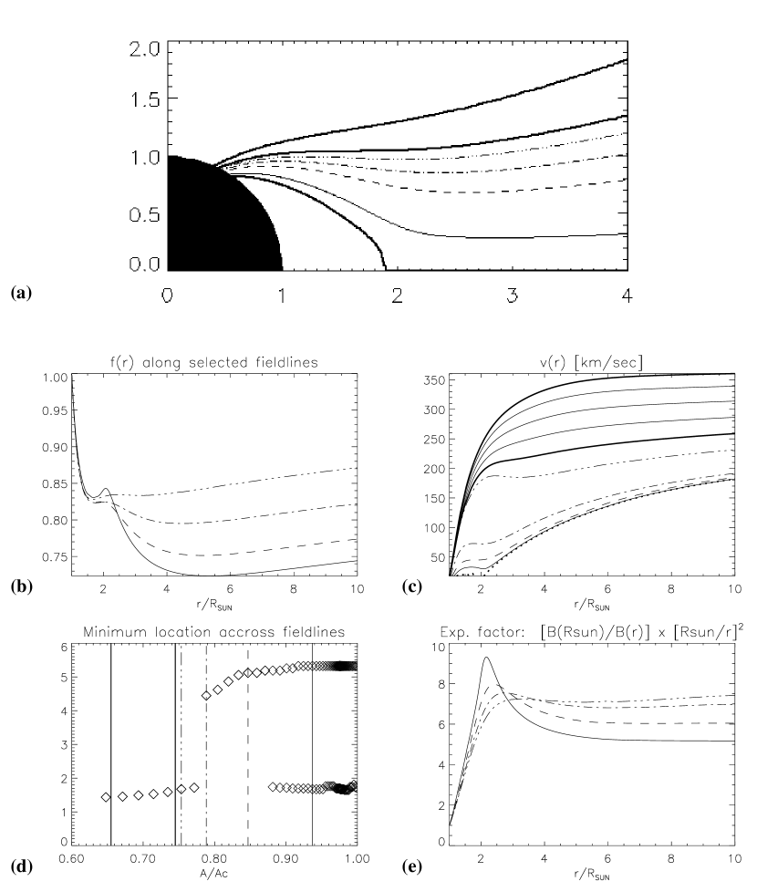
To show the transition between fast and slow wind more clearly, Figure The Effect of Proton Temperature Anisotropy on the Solar Minimum Corona and Wind shows various quantities along field lines near the fast-slow boundary (the same line styles are used in all panels). Panel (a) show the shapes of the field lines in the meridional plane. Panel (b) shows the function defined in equation (29) and plotted as function of radial distance for four field lines. Note that the triple-dot-dashed curve has a minimum at about 1.5 , whereas the full curve has two minima, one at 1.7 and another at 5.5 . As shown in §4.2, these minima indicate possible positions of the sonic point (). Panel (d) shows the radial positions of such minima as function of field-line variable . In general, a global solution of the wind equation (28) can be found only when the integration is started at the global minimum, i.e., the minimum with the lowest value of . Therefore, as we move from the triple-dot-dashed field lines to the dot-dashed line, there is a discontinuous jump in the height of the sonic point.
Figure The Effect of Proton Temperature Anisotropy on the Solar Minimum Corona and Windc shows the outflow velocity along field lines near the fast-slow boundary. The dotted curve in this panel is the wind solution along the last open field line, . As we move from the coronal hole into the streamer, the wind speed at large height closely follows the decrease in perpendicular temperature, which mainly occurs between the two full-thick profiles. However, a further decrease occurs at lower heights ( ) between the triple-dot-dashed and dot-dashed field lines due to the jump in height of the sonic point. We conclude that, unlike the terminal speed, the low-height behavior of is strongly affected by the height of the sonic point. Such a region of stagnated flow was found earlier by many authors (e.g., Wang Y.-M., 1994; Suess & Nerney, 1999, 2002; Chen & Hu, 2001).
Figure The Effect of Proton Temperature Anisotropy on the Solar Minimum Corona and Winde shows the non-radial expansion factor of the slow-wind flow tubes, , where in the field strength at the coronal base for each field line. Note that is a non-monotonic function of radius for these field lines. The peak in is due to the fact that these field lines pass close to the streamer cusp where . In contrast, increases monotonically for field lines in the coronal hole (not shown). It is remarkable to see that this “cusp effect” occurs at large distance from the cusp: the peak in occurs for all field lines within about 1 from the equatorial plane (see Figure The Effect of Proton Temperature Anisotropy on the Solar Minimum Corona and Winda). The triple-dot-dashed field line at which the peak in first develops is close to the field line where the jump in sonic-point height occurs. This is consistent with the suggestion by Suess & Nerney (1999, 2002), Chen & Hu (2002) and others that the existence of the slow wind is due to the non-monotonic behavior of . We suggest here that the decrease in perpendicular temperature as we approach the equatorial plane also plays an important role.
To determine whether the “cusp effect” is due to the effects of gas pressure on the expansion of the flow tubes, we computed a partially open potential magnetic field with the same photospheric boundary conditions [see equation (5)] and a thin current sheet in the equatorial plane for . The calculation is based on the work of Low (1986). First, the surface flux distribution is expressed in terms of four Legendre polynomials with = 1, 3, 5 and 7. Then the field is extrapolated into the corona using equations (B3) and (B4) of Low (1986) for = 1 and 3 (for = 5 and 7 the effect of the current sheet can be neglected). We found that has a peak for all open field lines that pass below the point = (3.0,1.4) , where is the distance from the rotation axis, and is the height above the equatorial plane. Therefore, the effect of the streamer cusp -located at the point = (1.95,0) - is present even in a potential field, and its spatial extent is similar to what was found in the numerical model (i.e., the effect is not due to the finite plasma ).
For the value of chosen in this paper ( = 0.7), the transition between fast and slow wind far from the Sun occurs at latitudes of . This is consistent with Ulysses observations taken at the time of cycle minimum (Suess et al., 1999). At lower heights, the low speeds in the streamer legs found in our model are consistent with UVCS measurements of outflow velocity using the Doppler dimming technique (Strachan et al., 2002). In a latitudinal scan at 2.33 , Strachan et al. (2002) found no measurable outflow velocity in the streamer ( km/s), but a steep rise in velocity occurs just beyond the bright streamer legs. The observed latitudinal half-width of the streamer at 2.33 , as defined by the points where the outflow velocity equals 100 km/s, is about . Our model predicts a half-width of . Therefore, the predicted width of the streamer is roughly consistent with observations at both large and small heights.
It should be noted that we use a realistic photospheric flux distribution that is peaked at the pole, [G], whereas Suess, Gary & Nerney (1999) and Chen & Hu (2001) assume a bipolar distribution, . For a given fraction of open magnetic flux, the assumed flux distribution has a significant effect on the size of the polar coronal hole, the latitudinal width of the streamer core, and the magnitude of the non-radial expansion factor. However, potential field models indicate that the spatial extent of the cusp effect is similar in the two cases.
6 Comparison with Visible Light and Ly Observations
The coronal density model can be used to predict the polarization brightness () of the visible light that is scattered by free electrons in the corona (Thomson scattering). The is an integral along the LOS (van de Hulst, 1950):
| (30) |
where is the distance along the LOS, is the projected radial distance from Sun center, is the true radial distance, is the Thomson scattering cross section, is the mean disk intensity, and is the limb darkening coefficient. The functions and are given by van de Hulst (1950). We used our axisymmetric model of the electron density distribution to compute synthetic images for various angles between the LOS and the solar equatorial plane. Figure The Effect of Proton Temperature Anisotropy on the Solar Minimum Corona and Wind shows the results for and ; the latter represents a view of the Sun from above the ecliptic plane. We have over-plotted selected field lines in the plane of the sky (white curves) and contours of the ratio of and its maximum value at the equatorial base (black curves). The equatorial streamer clearly stands out in the image with , but is less distinct for .
To compare these results with observations, Figure The Effect of Proton Temperature Anisotropy on the Solar Minimum Corona and Winda shows the radial profiles along the pole and equator, and Figure The Effect of Proton Temperature Anisotropy on the Solar Minimum Corona and Windb shows latitudinal profiles at three different heights ( = 1.15, 1.5 and 2.5 ). The full curves correspond to the edge-on view (). The symbols represent measurements obtained with the Mauna Loa Mark 3 coronagraph and LASCO/SOHO (Gibson et al., 1999; Guhathakurta et al., 1999) and with the visible-light channel on UVCS/SOHO (Cranmer et al., 1999). The data were obtained in 1996 July and August when the equatorial streamer belt is seen approximately edge-on (Raymond et al., 1997). Our model fits the observations quite well, although the predicted latitudinal width of the streamer at 2.5 is somewhat larger than observed. The dashed curve in Figure The Effect of Proton Temperature Anisotropy on the Solar Minimum Corona and Winda shows the radial profile along the pole for the out-of-ecliptic view (). Note that there is a large increase in compared to the edge-on view. This is due to the fact that the LOS crosses the enhanced density equatorial streamer, and is not representative of the available observations of the polar profile.
We also computed the intensity of the strongest UV coronal emission line, H I 1216 Å (Ly), which is formed almost entirely by resonant scattering of chromospheric Ly radiation by neutral hydrogen atoms in the corona (Noci, Kohl & Withbroe, 1987; Cranmer et al., 1999). The integrated intensity of the scattered Ly is
| (31) |
where measures distance along the LOS, is the neutral hydrogen density, is the radial distance from Sun center at any point along the LOS, is a geometric dilution factor, is the chromospheric intensity (in ) as function of frequency (in Hz), Hz is the line center frequency, is the Doppler shift, is the radial component of the outflow velocity, is the scattering profile of the coronal atoms (due to their thermal and non-thermal velocities), and is the Einstein coefficient. For a derivation of this expression and discussion of the relevant approximations, see Noci, Kohl & Withbroe (1987). The neutral hydrogen density is computed using the collisional ionization rates of Scholz & Walters (1991) and the recombination rates of Hummer (1994).
We computed Ly images for two different viewing angles, using densities, temperatures and velocities from the coronal model. The results are shown in Figure The Effect of Proton Temperature Anisotropy on the Solar Minimum Corona and Wind. Although these images look similar to those for polarization brightness, the Ly intensity is somewhat sensitive to the outflow velocity. This is shown more clearly in Figure The Effect of Proton Temperature Anisotropy on the Solar Minimum Corona and Wind where we plot the radial profiles of Ly intensity with and without the Doppler dimming effect (full and dashed curves, respectively). Note that there is a significant difference between predicted intensities with and without dimming for the polar region, but not for the equatorial region. Therefore, unlike measurements Ly intensities provide constraints on the outflow velocity in the acceleration region of the solar wind.
Figure The Effect of Proton Temperature Anisotropy on the Solar Minimum Corona and Wind also compares our model predictions with measurements from UVCS/SOHO. The diamonds represent measurements taken along the streamer axis, based on our reanalysis of data obtained on 1996 July 26 (Raymond et al., 1997). The triangles are measurements along the polar axis based on observations from November 1996 to April 1997 (Cranmer et al., 1999; Dobrzycka et al., 1999). Note that the predicted Ly intensities fit the observations quite well. This suggests that the model gives a reasonable representation of the velocity field in the inner part of the corona where the main acceleration of the solar wind takes place.
7 Discussion
We developed a stationary, axisymmetric MHD model for the global corona. The model includes a description of the temperature, density, velocity and magnetic field as function of latitude and radius up to 10 from sun center. The velocity and magnetic fields are obtained by solving the parallel and perpendicular force balance equations, including the effects of inertia, anisotropic gas pressure, gravity and Lorentz forces. The temperature models are based on observational data from UVCS/SOHO, and the magnetic flux distribution at the coronal base is taken from NSO/Kitt Peak synoptic maps. The model reproduces the main features of the global corona at the time of cycle minimum. We find that the high perpendicular temperature of the protons in the coronal hole plays a major role in driving the fast solar wind. In the streamer we find low outflow velocity and high plasma , consistent with earlier results (Suess et al., 1996; Wang A. H. et al., 1998a; Li et al., 1998).
In our model the wind equation (28) is solved separately for many field lines. The sonic point along each field line occurs at a minimum of the function that appears on the RHS of the wind equation [see equation (29)]. The transition from fast to slow wind occurs at an open field line characterized by , where is the boundary between open and closed fields. The value of was adjusted to obtain the correct latitudinal width of the slow-wind region both at large distance from the Sun (Suess et al., 1999) and in the corona at 2.33 (Strachan et al., 2002). In our model this transition is associated with two effects: (1) the decrease of proton perpendicular temperature as we approach the equatorial plane, and (2) the appearance of a peak in the non-radial expansion factor for field lines that pass close to the streamer cusp (“cusp effect”). The cusp effect is present at surprisingly large distances from the cusp ( ) and is present even in potential-field models, so it is not a consequence of finite plasma . The combination of decreasing temperature anisotropy and cusp effect causes the global minimum of (and therefore the sonic point) to occur well beyond the cusp, and produces low outflow velocity near the cusp. These results are consistent with the suggestion by Noci et al. (1997) that the slow wind is due to special properties of the geometric spreading along the open field lines that pass near the streamer core (also see Wang & Sheeley, 1990; Wang Y.-M., 1994; Wang Y.-M. et al., 1997b; Chen & Hu, 2001, 2002; Suess & Nerney, 1999, 2002).
Our model does not provide a physical explanation for the temperature decrease at the fast-slow boundary, and therefore cannot explain why the boundary occurs at . Understanding the physics of the fast-slow transition will require more detailed analysis of the energy balance of the coronal plasma, including the physical processes by which the temperature anisotropy of the protons is maintained. We speculate that proton perpendicular heating (by dissipation of transverse MHD waves) occurs in both the fast and slow winds, perhaps at roughly equal rates. However, the resulting temperature anisotropy may be quite different in the two cases. In the fast wind, proton-proton collisions are less frequent due to the lower density, so the deviations from Maxwellian velocity distributions are larger than in the slow wind. Clearly, to understand why the fast-slow transition occurs at will require multi-dimensional models of wave heating and energy balance such a those developed by Chen & Hu (2001).
References
- Allen, Habbal & Hu (1998) Allen, L. A., Habbal, S. R., & Hu, Y. Q. 1998, J. Geophys. Res., 103, 6551
- Allen (1973) Allen, C. W. 1973, Astrophysical Quantities (London: Athlone)
- Chen & Hu (2001) Chen, Y., & Hu, Y. Q. 2001, Sol. Phys., 199, 371
- Chen & Hu (2002) Chen, Y., & Hu, Y. Q. 2002, Ap&SS, 282, 447
- Cranmer (2002) Cranmer, S. R. 2002, in Proc. of 11th SOHO Symposium, From Solar Min to Max: Half a Solar Cycle with SOHO, ed. A. Wilson, ESA SP-508 (Noordwijk: ESA), 361
- Cranmer et al. (1999) Cranmer, S. R., Kohl, J. L., Noci, G., Antonucci, E., Tondello, G., Huber, M. C. E., Strachan, L., et al. 1999, ApJ, 511, 481
- Cuperman et al. (1993) Cuperman, S., Bruma, C., Detman, T., & Dryer, M. 1993, ApJ, 404, 356
- Cuperman et al. (1990) Cuperman, S., Ofman, L., & Dryer M. 1990, ApJ, 350, 846
- Dobrzycka et al. (1999) Dobrzycka, D., Cranmer S. R., Panasyuk, A. V., Strachan L., & Kohl, J. L. 1999, J. Geophys. Res., 104, 9791
- Dusenbery & Hollweg (1981) Dusenbery, P. B., & Hollweg, J. V. 1981, J. Geophys. Res., 86, 153
- Frazin, Cranmer & Kohl (2003) Frazin, R. A., Cranmer, S. R., and Kohl, J. L. 2003, ApJ, submitted
- Frazin (2002) Frazin, R. A. 2002, Empirical Constraints on O5+ Outflows and Velocity Distributions in a Solar Minimum Coronal Streamer, Ph.D. Thesis, The University of Illinois at Urbana-Champaign
- Gibson et al. (1999) Gibson, S. E., Fludra, A., Bagenal, F., Biesecker, D., Del Zanna, G., & Bromage, B. 1999, J. Geophys. Res., 104, 9691
- Gibson (2001) Gibson, S. E. 2001, Space Sci. Rev., 97, 69
- Guhathakurta et al. (1999) Guhathakurta, M., Fludra, A., Gibson, S. E., Biesecker, D., & Fisher, R. 1999, J. Geophys. Res., 104, 9801
- Guhathakurta, Holzer & MacQueen (1996) Guhathakurta, M., Holzer, T. E., & MacQueen, R.M. 1996, ApJ, 458, 817
- Habbal et al. (1997) Habbal, S. R., Woo, R., Fineschi, S., O’Neal, R., Kohl, J., Noci, G., & Korendyke, C. 1997, ApJ, 489, L103
- Hu & Habbal (1999) Hu, Y. Q., & Habbal, S. R. 1999, J. Geophys. Res., 104, 17045
- Hummer (1994) Hummer, D. G. 1994, MNRAS, 268, 109
- Isenberg & Hollweg (1983) Isenberg, P. A., & Hollweg, J. V. 1983, J. Geophys. Res., 88, 3293
- Ko et al. (1997) Ko, Y.-K., Fisk, L. A., Geiss, J., Gloeckler, G., Guhathakurta, M. 1997, Sol. Phys., 171, 345
- Kohl et al. (1995) Kohl, J. L., Esser, R., Gardner, L. D., Habbal, S., Daigneau, P. S., Dennis, E. F., Nystrom, G. U., et al. 1995, Sol. Phys., 162, 313
- Kohl et al. (1997) Kohl, J. L., Noci, G., Antonucci, E., Tondello, G., Huber, M. C. E., Gardner, L. D., Nicolosi, P., Strachan, L., et al. 1997, Sol. Phys., 175, 613
- Kohl et al. (1998) Kohl, J. L., Noci, G., Antonucci, E., Tondello, G., Huber, M. C. E., Cranmer, S. R., Strachan, L., et al. 1998, ApJ, 501, L127
- Kohl, Strachan & Gardner (1996) Kohl, J. L., Strachan, L., & Gardner, L. D. 1996, ApJ, 465, L141
- Landi et al. (2001) Landi, E., Doron, R., Feldman, U., & Doschek, G. A. 2001., ApJ, 556, 912
- Li et al. (1998) Li, J., Raymond, J. C., Acton, L. W., Kohl, J. L., Romoli, M., Noci, G., & Naletto, G. 1998, ApJ, 506, 431L
- Linker, Van Hoven & Schnack (1990) Linker, J. A., Van Hoven, G., and Schnack, D. D. 1990, J. Geophys. Res.17, 2281
- Lionello, Linker & Mikic (2001) Lionello, R., Linker, J. A., & Mikic, Z. 2001, ApJ, 546, 542
- Low (1986) Low, B. C. 1986, ApJ, 310, 953
- Marsh et al. (1982) Marsh, E., Muhlhauser, K.-H., Rosenbauer, H., Schwenn, R., & Neubauer, F. M. 1982, J. Geophys. Res., 86, 9199
- Munro & Jackson (1977) Munro, R. H., & Jackson, B. V. 1977, ApJ, 213, 874
- Newkirk (1967) Newkirk, G. A., Jr. 1967, ARA&A, 5, 213
- Noci et al. (1997) Noci, G., Kohl, J. L., Antonucci, E., Tondello, G., Huber, M. C. E., Fineschi, S., Gardner, L. D., et al. 1997, in Proc. Fifth SOHO Workshop: The Corona and Solar Wind Near Minimum Activity, ed. A. Wilson, ESA SP-404 (Noordwijk: ESA), 75
- Noci, Kohl & Withbroe (1987) Noci, G., Kohl, J. L., & Withbroe, G. L. 1987, ApJ, 315, 706
- Olsen & Leer (1996) Olsen, E. L., & Leer, E. 1996, ApJ, 462, 982
- Olsen, Leer & Holzer (1994) Olsen, E. L., Leer, E., & Holzer, T. 1994, ApJ, 420, 913
- Phillips et al. (1995) Phillips, J. L., Bame, S. J., Barnes, A., Barraclough, B. L., Feldman, W. C., Goldstein, B. E., Gosling, J. T., et al. 1995, Geophys. Res. Lett., 22, 3301
- Pilipp et al. (1987) Pilipp, W. G., Muehlhaeuser, K.-H., Miggenrieder, H., Montgomery, M. D., Rosenbauer, H. 1987, J. Geophys. Res., 92, 1075
- Pneuman & Kopp (1971) Pneuman, G., & Kopp, R. A. 1971, Sol. Phys., 18, 258
- Press, et al. (1992) Press, W. H., Teucholsky, S. A., Vetterling, W. T., & Flannery, B. P. 1992, Numerical Recipes in Fortran: The Art of Scientific Computing, 2nd Edition (Cambridge University Press), 413
- Raymond et al. (1997) Raymond, J. C., Kohl, J. L., Noci, G., Antonucci, E., Tondello, G., Huber, M. C. E., Gardner, L. D., Nicolosi, P., et al. 1997, Sol. Phys., 175, 645
- Riley, Linker & Mikic (2001) Riley, P., Linker, J. A., & Mikic, Z. 2001, J. Geophys. Res., 106, 15889
- Saito et al. (1977) Saito, K., Poland, A. I., & Munro., R. H. 1977, Sol. Phys., 55, 121
- Scholz & Walters (1991) Scholz, T. T., & Walters, H. R. J. 1991, ApJS, 380, 302
- Sheeley et al. (1997) Sheeley, N. R., Jr., Wang, Y.-M., Hawley, S. H., Brueckner, G. E., Dere, K. P., Howard, R. A., Koomen, M. J., et al. 1997, ApJ, 484, 472
- Sittler & Guhathakurta (1999) Sittler, E. C., Jr., & Guhathakurta, M. 1999, ApJ, 523, 812
- Steinolfson, Suess & Wu (1982) Steinolfson, R. S., Suess, S. T., & Wu, S. T. 1982, ApJ, 255, 730
- Strachan et al. (2002) Strachan, L., Suleiman, R., Panasyuk, A. V., Biesecker, D. A., & Kohl, J. L. 2002, ApJ, 571, 1008
- Suess & Nerney (1999) Suess, S. T., & Nerney, S. F. 1999, in Proc. 9th European Meeting on Solar Physics, Magnetic Fields and Solar Processes, ed. A. Wilson, ESA SP-44 (Noordwijk: ESA), 1101
- Suess & Nerney (2002) Suess, S. T., & Nerney, S. F. 2002, ApJ, 565, 1275
- Suess, Gary & Nerney (1999) Suess, S. T., Gary, G. A., & Nerney, S. F. 1999b, in Proc. of the Ninth International Solar Wind Conference, eds. S. R. Habbal, R. Esser, J. V. Hollweg, & P. A. Isenberg, AIP Conf. Proc., Vol. 471, 247
- Suess et al. (1999) Suess, S. T., Poletto, G., Corti, G., Simnett, G., Noci, G., Romoli, R., Kohl, J., & Goldstein, B. 1999, Space Sci. Rev., 87, 319
- Suess et al. (1996) Suess, S. T., Wang, A.-H., & Wu, S. T. 1996, J. Geophys. Res., 101, 19957
- Tu & Marsch (1997) Tu, C.-Y., & Marsch, E. 1997, Sol. Phys., 171, 363
- van de Hulst (1950) van de Hulst, H. C. 1950, Bull. Astron. Inst. Neth., 11, 135
- Vásquez, Raymond & van Ballegooijen (1999) Vásquez, A. M., Raymond, J. C., & van Ballegooijen, A. A. 1999, Space Sci. Rev., 87, 335
- Vásquez, van Ballegooijen & Raymond (1999) Vásquez, A. M., van Ballegooijen, A. A., & Raymond, J. C. 1999, in Proc. of the Ninth International Solar Wind Conference, eds. S. R. Habbal, R. Esser, J. V. Hollweg, & P. A. Isenberg, AIP Conf. Proc., Vol. 471, 243
- Wang A. H. et al. (1993) Wang, A. H., Wu, S. T., Suess, S. T., & Poletto, G. 1993, Sol. Phys., 147, 55
- Wang A. H. et al. (1998a) Wang, A. H., Wu, S. T., Suess, S. T., & Poletto, G. 1998a, J. Geophys. Res., 103, 1913
- Wang Y.-M. (1994) Wang, Y.-M. 1994, ApJ, 437, L67
- Wang & Sheeley (1990) Wang, Y.-M., & Sheeley, N. R., Jr. 1990, ApJ, 355, 726
- Wang Y.-M. et al. (1997a) Wang, Y.-M., Sheeley, N. R., Jr., Howard, R. A., Kraemer, J. R., Rich, N. B., Andrews, M. D., Brueckner, G. E., et al. 1997a, ApJ, 485, 875
- Wang Y.-M. et al. (1997b) Wang, Y.-M., Sheeley, N. R., Jr., Phillips, J. L., & Goldstein, B. E. 1997b, ApJ, 488, L51
- Wang Y.-M. et al. (1998b) Wang, Y.-M., Sheeley, N. R., Jr., Walters, J. H., Brueckner, G. E., Howard, R. A., Michels, D. J., Lamy, P. L., Schwenn, R., Simnett, G. M. 1998b, ApJ, 498, L165
- Washimi, Yoshino & Ogino (1987) Washimi, H., Yoshino, Y. and Ogino, T. 1987, J. Geophys. Res., 14, 487
- Wilhelm et al. (1998) Wilhelm, K., Marsch, E., Dwivedi, B. N., Hassler, D. M., Lemaire, Ph., Gabriel, A. H., Huber, M. C. E. 1998, ApJ, 500, 1023
- Withbroe et al. (1982) Withbroe, G. L., Kohl, J. L., Weiser, H., & Munro, R. H. 1982, Space Sci. Rev., 33, 17
- Yeh & Pneuman (1977) Yeh, T., & Pneuman, G. W. 1977, Sol. Phys., 54, 419
Electron density profiles derived from Skylab observations for the pole (thin curve) and the equator (thick curve).
Temperature profiles derived from coronal observations, for the pole and the equator.
Photospheric magnetic field as function of latitude at the time of the last cycle minimum (July 1996). The diamonds are measurements from Kitt Peak synoptic maps. The full curve is a fit to the data.
Sketch of the dipolar configuration.
The function used for interpolating temperatures between pole and equator.
Magnetic field and plasma pressure for the first iteration (top) and for the final model (bottom). The thin curves are magnetic field lines (contours of ), and the thick curves are contours of .
Outflow velocity in the meridional plane. The brightness level increases with magnitude of the outflow speed, , as shown by the scale on the left side of the figure ( in km/s). The solar rotation axis is along the left axis of the plot, and the solar surface is indicated by the thick semi-circle. The white curves are selected field lines labeled with their value of .
Various wind properties as function of field-line variable . Top panel: temperature anisotropy at . Middle panel: radius of sonic point where (in ). Bottom panel: wind speed at (in km/s). The thin solid vertical line in each panel indicates the field line where the latitudinal temperature gradient is largest, and the thick vertical lines indicate the width of the transition (). The dot-dashed vertical line indicates the field line at which there is a sudden transition in the radius of the sonic point.
Transition between fast and slow wind. (a) Shape of various field lines in the meridional plane. (b) Functions that appear on the RHS of the wind equation (28) for different field lines. (c) Outflow velocity along field lines. The dotted curve corresponds to the last open field line, . (d) Radial positions of the mimima of as function of field-line variable (diamonds). The vertical lines show the -values of the field lines shown in other panels. (e) Non-radial expansion factors for different field lines. The same line styles are used in all panels.
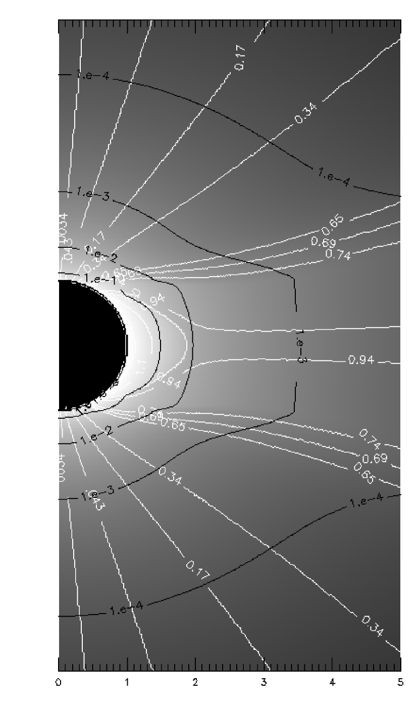
Images of visible light polarization brightness () as predicted from the coronal model. Black curves are contours of , where is the value of at the coronal base. The white curves are selected field lines in the plane of the sky (labeled by ). The dark semi-circle represents the solar disk.
Left panel: Visible-light polarization brightness of the corona, , as function of radial distance from sun center. The solid curves show the predicted equatorial (thick) and polar (thin) profiles for an edge-on view. The dashed curve is the predicted polar profile for a view from above the ecliptic plane (). The symbols are measurements for the pole (triangles) and equator (diamonds) from Gibson et al. (1999), Guhathakurta et al. (1999), and Cranmer et al. (1999). Right panel: Predicted polarization brightness as function of co-latitude at projected radii of 1.15, 1.5, and 2.5 . The symbols are corresponding measurements from the above-cited references.
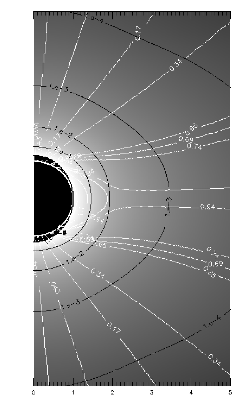
Images of Ly intensity as predicted from the coronal model. The black curves are contours of , where is the maximum value of at the coronal base. The white curves are selected field lines in the plane of the sky (labeled with ). The dark semi-circle represents the solar disk.
Radial profiles of Ly intensity . The solid curves are the predicted intensity along the pole (thin solid curve) and along the equator (thick solid curve) for the edge-on view (). The dashed curves are the predicted profiles without Doppler dimming [i.e., with in equation (31)]. The triangles and diamonds are intensity measurements from UVCS/SOHO for the pole and equator, respectively (see text).
| , | ,, | ||
|---|---|---|---|
| at Pole | at Pole | at Equator | |
| K | K | K | |
| K | 0. | 0. | |
| 0. | 0. | 0.1 | |
| 0.23 | 0.47 | 0.33 | |
| 0.7 | 0.7 | 0.55 | |
| 6.6 | 6.6 | 6.6 | |
| 1 |