Abstract

”The purpose of numerical models is not numbers but insight.” (Hamming) In the spirit of this adage, and of Don Cox’s approach to scientific speaking, we discuss the questions that the latest generation of numerical models of the interstellar medium raise, at least for us. The energy source for the interstellar turbulence is still under discussion. We review the argument for supernovae dominating in star forming regions. Magnetorotational instability has been suggested as a way of coupling disk shear to the turbulent flow. Models make evident that the unstable wavelengths are very long compared to thermally unstable wavelengths, with implications for star formation in the outer galaxy and low surface brightness disks. The perennial question of the factors determining the hot gas filling factor in a SN-driven medium remains open, in particular because of the unexpectedly strong turbulent mixing at the boundaries of hot cavities seen in the models. The formation of molecular clouds in the turbulent flow is also poorly understood. Dense regions suitable for cloud formation clearly form even in the absence of self-gravity, although their ultimate evolution remains to be computed.

The Turbulent Interstellar Medium: Insights and Questions from Numerical Models

Turbulent ISM

1 Questions about Turbulence

Numerical models often yield insight into the behavior of a physical system long before they can give quantitative results. In this contribution we review possible answers to three major questions about turbulence, relying on a combination of general energetic arguments and numerical models.

The first question is, “What provides the energy to drive the turbulent flow?” Many sources have been proposed, but few have the required energy to counteract dissipation in the interstellar medium. Supernovae (SNe) seem likely to be the primary driver in parts of galaxies where star formation occurs, while the magnetorotational instability (MRI) may couple the gas to galactic rotational shear in other parts of galaxies.

The second question is, “How does the driving shape the flow?” Most of the energy lies at the driving scale, so the large-scale structure is determined quite directly by the driving mechanism. Turbulent compression may be as important as thermodynamic phases in determining the pressure at any particular point in the ISM, as well as in determining the filling factor of the hot gas.

The last question, of interest to understanding the rate of star formation from the ISM, is “How do molecular clouds form in this flow?” Turbulent compression and self-gravity both appear as possible mechanisms, but cannot yet be definitively distinguished.

2 What Drives the Turbulence?

Maintenance of observed motions appears to depend on continued driving of the turbulence, which has kinetic energy density $e=(1/2)\rho v_{\rm rms}^{2}$. Mac Low [12, 13] estimates that the dissipation rate for isothermal, supersonic turbulence is

$$\dot{e} \simeq -(1/2)\rho v_{\rm rms}^{3}/L_{\rm d}$$

$$= -(3\times 10^{-27}\,\mbox{erg}\,\mbox{cm}^{-3}\,\mbox{s}^{-1})\left(\frac{n}{1\,\mbox{cm}^{-3}}\right)\left(\frac{v_{\rm rms}}{10\,\mbox{km}\,\mbox{s}^{-1}}\right)^{3}\left(\frac{L_{\rm d}}{100\,\mbox{pc}}\right)^{-1},$$

where $L_{\rm d}$ is the driving scale, which we have somewhat arbitrarily taken to be 100 pc (though it could well be smaller, or a broad range), and we have assumed a mean mass per particle $\mu=2.11\times 10^{-24}$ g. The dissipation time for turbulent kinetic energy $\tau_{\rm d}=e/\dot{e}\simeq L_{\rm d}/v_{\rm rms},$ which is just the crossing time for the turbulent flow across the driving scale [8]. What then is the energy source for this driving? We here review the energy input rates for the most plausible mechanisms, feedback from massive stars, particularly SNe, and magnetorotational instabilities. A more extensive discussion covering a number of other possibilities as well is given by Mac Low & Klessen [15].

An energy source for interstellar turbulence that has long been considered is shear from galactic rotation [9]. However, the question of how to couple from the large scales of galactic rotation to smaller scales remained open. Sellwood & Balbus [20] suggested that the MRI [5, 6] could couple the large and small scales efficiently. The instability generates Maxwell stresses (a positive correlation between radial $B_{R}$ and azimuthal $B_{\Phi}$ magnetic field components) that transfer energy from shear into turbulent motions at a rate

$$\dot{e}=-T_{R\Phi}(d\Omega/d\ln R)=T_{R\Phi}\Omega,$$ (2)

where the last equality holds for a flat rotation curve [20]. Numerical models suggest that the Maxwell stress tensor $T_{R\Phi}\simeq 0.6B^{2}/(8\pi)$ [11]. For the Milky Way, the standard value of the rotation rate $\Omega=(220\mbox{ Myr})^{-1}=1.4\times 10^{-16}\mbox{ rad s}^{-1}$, so the MRI can contribute energy at a rate

$$\dot{e}=(3\times 10^{-29}\,\mbox{erg}\,\mbox{cm}^{-3}\,\mbox{s}^{-1})\left(\frac{B}{3\mu\mbox{G}}\right)^{2}\left(\frac{\Omega}{(220\,\mbox{Myr})^{-1}}\right).$$ (3)

For parameters appropriate to the Hi disk of a sample small galaxy, NGC 1058, including $\rho=10^{-24}\,$g cm^-3, Sellwood & Balbus [20] find that the magnetic field required to produce the observed velocity dispersion of 6 km s^-1 is roughly 3 $\mu$G, a reasonable value for such a galaxy. This instability may provide a base value for the velocity dispersion below which no galaxy will fall. If that is sufficient to prevent collapse, little or no star formation will occur, producing something like a low surface brightness galaxy with large amounts of Hi and few stars. This may also apply to the outer disk of our own Milky Way and other star-forming galaxies.

In active star-forming galaxies, massive stars probably dominate the driving at radii where they form. They could do so through ionizing radiation and stellar winds from O stars, or clustered and field SN explosions, predominantly from B stars no longer associated with their parent gas. Mac Low & Klessen [15] demonstrate that ionizing radiation is unlikely to dominate the kinetic energy budget, despite the large amount of energy going into heating and ionization. The total energy input from the line-driven stellar wind over the main-sequence lifetime of an early O star can equal the energy from its SN explosion, and the Wolf-Rayet wind can be even more powerful. However, the mass-loss rate from stellar winds drops as roughly the sixth power of the star’s luminosity, while the powerful Wolf-Rayet winds [19] last only $10^{5}$ years or so, so only the very most massive stars contribute substantial energy from stellar winds. The energy from SN explosions, on the other hand, remains nearly constant down to the least massive star that can explode. As there are far more lower-mass stars than massive stars, SN explosions inevitably dominate over stellar winds after the first few million years of the lifetime of an OB association.

To estimate the energy input rate from SNe, we begin with a SN rate for the Milky Way of (50 yr)^-1, which agrees well with the estimate in equation (A4) of McKee [17]). If we take the scale height of SNe $H_{c}\simeq 100$ pc and a star-forming radius $R_{sf}\simeq 15$ kpc, we can compute the energy input rate from SN explosions with energy $E_{SN}=10^{51}\,$erg to be

$$\dot{e} = \frac{\sigma_{SN}\eta_{SN}E_{SN}}{\pi R_{sf}^{2}H_{c}}$$

$$= (3\times 10^{-26}\mbox{ erg s${}^{-1}$ cm}^{-3})\left(\frac{\eta_{SN}}{0.1}\right)\left(\frac{\sigma_{SN}}{1\mbox{ SNu}}\right)\left(\frac{H_{c}}{100\mbox{ pc}}\right)^{-1}\times$$

$$\times \left(\frac{R_{sf}}{15\mbox{ kpc}}\right)^{-2}\left(\frac{E_{SN}}{10^{51}\mbox{ erg}}\right).$$

The efficiency of energy transfer from SN blast waves to the interstellar gas $\eta_{SN}$ depends on the strength of radiative cooling in the initial shock, which will be much stronger in the absence of a surrounding superbubble (e.g. [10]). Substantial amounts of energy can escape in the vertical direction in superbubbles as well, however. The scaling factor $\eta_{SN}\simeq 0.1$ used here was derived by Thornton et al. [22] from detailed, 1D, numerical simulations of SNe expanding in a uniform ISM. It can alternatively be drawn from momentum conservation arguments, comparing a typical expansion velocity of 100 km s^-1 to typical interstellar turbulence velocity of 10 km s^-1. Multi-dimensional models of the interactions of multiple SN remnants (e.g. [1]) are required to better determine the effective scaling factor.

SN driving appears to be powerful enough to maintain the turbulence even with the dissipation rates estimated in Eq. (2). It provides a large-scale self-regulation mechanism for star formation in disks with sufficient gas density to collapse despite the velocity dispersion produced by the MRI. As star formation increases in such galaxies, the number of OB stars increases, ultimately increasing the SN rate and thus the velocity dispersion, which restrains further star formation.

3 How Does Driving Shape the ISM?

We now turn to the question of how these different driving mechanisms determine the structure of the ISM. Clearly, different mechanisms yield different results.

To study the MRI, we used a parallel MHD code integrating $\ln\rho$ rather than density $\rho$ to handle strong density contrasts [7], with shearing sheet horizontal boundary conditions implemented. The preliminary models shown here were run at $64\times 64\times 128$ zones on an $0.5\times 0.5\times 1$ kpc grid, with the ISM in vertical hydrostatic equilibrium with scale height $H=250$ pc initially, and an initially vertical magnetic field with thermal to magnetic pressure ratio $\beta=1000$. The initial wavelength of maximum instability was then 80 pc. Runs were extended to 10 orbits, or 2.5 Gyr. Radiative cooling was included based on an equilibrium ionization cooling curve including thermal instability below $10^{4}$ K, and heating proportional to density was chosen to exactly balance the cooling in the initial model. We ran models initially in thermally stable and unstable regimes.

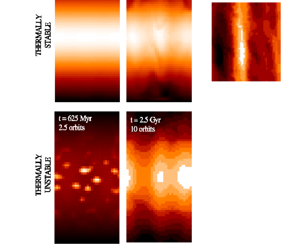
Figure 1: Log of density on vertical cuts through 3D shearing sheet models of MRI at times given. Top: thermally stable models, including a horizontal cut through the midplane of the final model; Bottom: thermally unstable models, showing the action of the MRI on the cooled clumps.

In Figure 1 we show the development of the MRI in these regimes. In the thermally stable regime, factor of 2–3 column density contrasts through the disk are created by the instability. In the thermally unstable regime, the thermal instability acts quickly to clump the gas, but after multiple orbits the MRI adds sufficient velocity dispersion to heat the gas and distribute it more uniformly. Rather more substantial column density contrasts still occur. Comparison with observed Hi disks outside of the star-forming region should be revealing of whether this mechanism is in fact maintaining their velocity dispersion.

Numerical models of the SN-driven ISM suggest that the hot gas filling factor $f$ is closer to the value $f\sim 0.2$ [1, 2, 3] predicted by Slavin & Cox [21] than to the values close to unity predicted by McKee & Ostriker [18]. Why is this? McKee & Ostriker [18] assumed a two-phase medium with cold, dense clouds embedded in a uniform density, warm, intercloud medium. Hot SN remnants then expanded into this medium. Was the cooling within the SN remnants underestimated because turbulent mixing was approximated with mass loading from the clumps overrun by the remnants, or was the effective external density underestimated by the two-phase model?

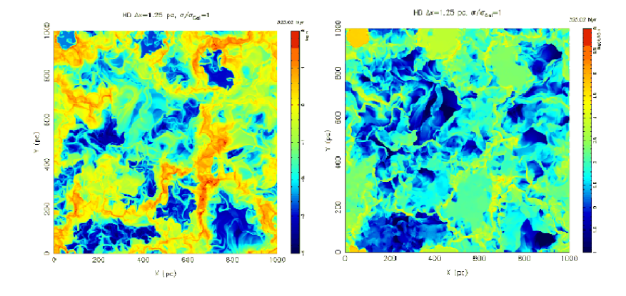
Figure 2: Cuts through the midplane of the SN-driven model run at finest resolution of 1.25 pc. Left: Density; Right: Pressure.

To study the SN-driven ISM we used an adaptive mesh refinement code described by Avillez & Mac Low [4], with a $1\times 1\times 20$ kpc grid set up as described in Avillez [1], with a SN rate equal to the galactic value.

Figure 2 shows that the pressures vary widely [14], so that no simple two-phase medium can actually form. Instead, the densities cover a broad range continuously, as shown in Figures 2 and 3.

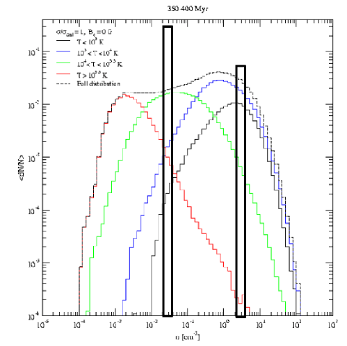
Figure 3: Probability distribution function of density in the midplane of the SN-driven model. The two-phase medium assumed by McKee & Ostriker [18] is shown schematically by the thick black rectangles.

This continuous distribution of density may act to impede the expansion of SN remnants more effectively than the warm intercloud medium with cold embedded clouds shown schematically in Figure 3.

On the other hand, Avillez & Mac Low [4] demonstrated using a tracer field that mixing occurs quite efficiently in the hot regions. In Figure 2 widespread turbulent mixing at the edges of shells and supershells can be seen. This could substantially enhance the density in the hot interiors, thus enhancing the radiative cooling, which is proportional to $\rho^{2}$. However, a quantitative test of how well or poorly this turbulent mixing was modeled by the model of SN remnants overrunning conductively evaporating clouds used by McKee & Ostriker [18] remains to be done.

4 How Do Molecular Clouds Form in the Turbulent ISM?

Molecular clouds are high-density objects, with much of their mass at densities of $10^{3-5}$ cm^-3. With typical temperatures of order 10 K, their pressures are an order of magnitude or more above the average ISM pressure. It has usually been argued that these high pressures must be caused by self-gravity, since they would otherwise explode. However, turbulent ram pressure in a SN-driven ISM produces high-density, high-pressure regions even in the absence of self-gravity, as shown in Figure 4. These may provide the sites for the formation of at least some molecular clouds, especially ones that do not show vigorous, efficient, star formation.

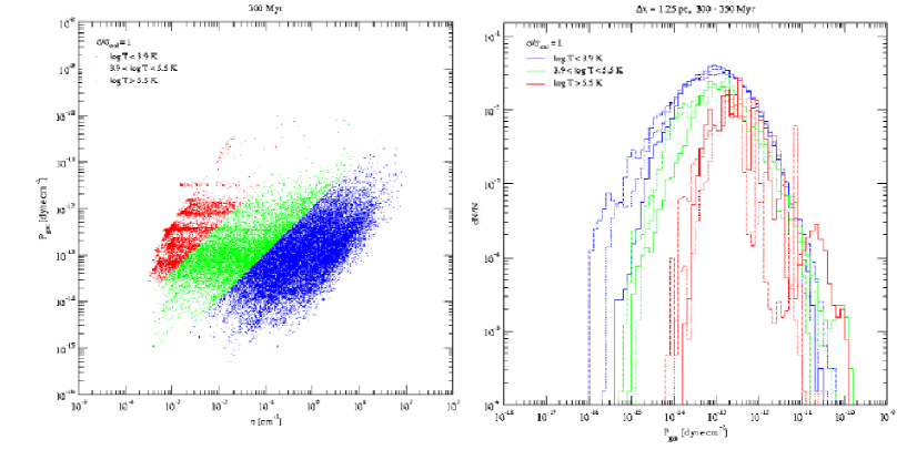
Figure 4: Left: Scatter plot of pressure vs. density in the midplane of the SN-driven model showing occupation of high-pressure, high-density region associated with molecular clouds. Right: Volume-weighted probability distribution function of pressure in the same model. Note that the small volumes occupied by high-density, cold gas have large mass.

5 Discussion

Gaensler: We know from observations of scattering & scintillation that there is turbulence in the warm ionized phase of the ISM. Since we expect expanding SN remnants to sweep up neutral shells, can SN remnants still drive the turbulence seen in ionized gas? What sort of a contribution do ionization fronts make to turbulence in ionized gas? Mac Low: In our models, most of the turbulence comes from the interaction of multiple shells. Diffuse ionizing radiation will ionize some of that gas, producing diffuse, turbulent, ionized gas. H ii regions also contribute, of course. In Mac Low & Klessen [15] we use results from Matzner [16] to argue that H ii region expansion is only a minor (¡ 1%) contributor to ISM kinetic energy.

Heiles: You emphasized the breadth of the pressure distribution. But it’s really not more than an order of magnitude, right? Mac Low: That is true for the volume-weighted FWHM. However, a mass-weighted view shows that a substantial fraction of the mass is at the high-density end.