Gravitational microlensing of quasar broad line regions at large optical depths

Abstract

Recent estimates of the scale of structures at the heart of quasars suggest that the region responsible for the broad line emission are smaller than previously thought. With this revision of scale, the broad line region is amenable to the influence of gravitational microlensing. This study investigates the influence on microlensing at high optical depth on a number of current models of the Broad Line Region (BLR). It is found that the BLR can be significantly magnified by the action of microlensing, although the degree of magnification is dependent upon spatial and kinematic structure of the BLR. Furthermore, while there is a correlation between the microlensing fluctuations of the continuum source and the BLR, there is substantial scatter about this relation, revealing that broadband photometric monitoring is not necessarily a guide to microlensing of the BLR. The results of this study demonstrate that the spatial and kinematic structure within the BLR may be determined via spectroscopic monitoring of microlensed quasars.

1 Introduction

Quasars are amongst the most luminous sources in the universe. At cosmological distances, their relatively small size ensures the regions responsible for producing the various spectral line components remains effectively unresolved with modern telescopes. Gravitational microlensing, however, can significantly magnify the inner regions, providing clues to the various scales of structure located at the heart of quasars, giving some of the best estimates of the scale of the central continuum emitting region (e.g. Jaroszynski, Wambsganss, & Paczynski, 1992; Yonehara, 1999; Wyithe, Webster, Turner, & Mortlock, 2000), as well as offering the possibility of probing the nature of other quasar small scale structure  (Belle & Lewis, 2000; Wyithe & Loeb, 2002).

The degree of microlensing magnification is dependent upon the scale size of the source, with smaller sources being more susceptible to large magnifications (e.g. Wambsganss & Paczynski, 1991). While the continuum emitting region of a quasar is small enough to undergo significant magnification, the more extensive line emitting regions, specifically the BLR with a scale length of 0.1-a few pc, were considered to be too large to suffer substantial magnification. Nemiroff (1988) undertook a study to determine the degree of microlensing of various models of the BLR, examining the influence of a single microlensing mass in front of the emission region. When considering microlensing in multiply imaged quasars, however, many stars are expected to influence the light beam of a distant source, and these combine in a very non-linear fashion and the single star approximation is a poor one (e.g. Wambsganss et al., 1990). Schneider & Wambsganss (1990) considered the microlensing of a BLR at substantial optical depth. These studies found that while gravitational microlensing did result in the modification of the BLR emission line profiles, the overall magnification of the region was small, typically less than 30%.

These microlensing studies employed estimates of the size of the quasar BLR based upon simple ionization models [see Davidson & Netzer (1979)]. Reverberation mapping, however, provides a more direct measure of the geometry of the BLR and early studies suggested these simple ionization models had over estimated the scale of the BLR by roughly an order of magnitude (e.g. Peterson et al., 1985), prompting a revision of BLR physics (Rees, Netzer, & Ferland, 1989). More recent reverberation measurements have refined the size of the BLRs in active galaxies, finding it to be $\sim 10^{-4}$pc in low luminosity AGN, up to $\sim 10^{-1}$pc in luminous quasars, with the size of the BLR scaling with the luminosity of the quasar, such that $R_{BLR}\propto L^{0.7}$ (Wandel, Peterson, & Malkan, 1999; Kaspi et al., 2000). Furthermore, these results demonstrate the BLR possesses a stratified structure, with high ionization lines being an order of magnitude smaller than lower ionization lines. Following this discovery, Abajas et al. (2002) reexamined the question of the microlensing of the BLR region in light of this revised scale. Undertaking an analysis similar to Nemiroff (1988), they considered the influence of a single microlensing mass located in the BLR, finding that significant modification of the BLR line profile results.

Figure 1: The Einstein Radius for a solar mass star for lenses at $z=0.1,0.4,0.7$ & $1.0$, denoted by the location of the start of each curve, for sources at a range of redshifts. The panels on the right hand size present the expects size of the high ionization (column topped with Hi) and low ionization (Lo) BLRs, for the denoted absolute magnitudes.

As with the approach of Nemiroff (1988), the study of Abajas et al. (2002) is a poor representation of microlensing at significant optical depth, the situation for multiply imaged quasars. This paper, therefore, also examines the question of microlensing of the BLR, extending the previous work of Abajas et al. (2002) into the higher optical depth regime. The approach to this question is described in Section 2, whereas the results are discussed in Section3. The conclusions to this study are presented in Section 4.

2 Method

2.1 Microlensing Maps

The known number of multiply imaged quasars has been steadily growing in recent years (Muñoz et al., 1998). For the majority of these, little temporal data has been obtained and so this study focuses upon the quadruple quasar Q2237+0305, the first system in which microlensing was confirmed (Irwin et al., 1989). The microlensing parameters, the surface mass density $\sigma$ and the shearing due to external mass $\gamma$, were taken from the modeling of Schmidt et al. (1998); for images C and D the values for $(\sigma,\gamma)$ were $(0.69,0.71)$ and $(0.59,0.61)$ respectively. Images A and B have similar microlensing parameters, chosen to be $(0.36,0.41)$ for the purpose of this study. These microlensing parameters may seem quite specific and hence not applicable to the population of lensed quasars in general. However, for multiply imaged systems the microlensing parameters must be substantial and hence the simulations in this paper can be taken as representative.

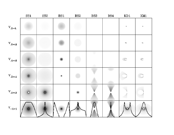
Figure 2: The appearance of each of the BLR models as a function of velocity. The models are presented vertically, with the model label given at the top of each column; the details of the models are given in Table 1, with the SS models representing spherical shells of clouds, the BS models being biconical shells, where as the KD & KM models are thin disks. The five velocity slices consider the range from 0 to 1 in units of 0.2; as the models are symmetric in velocity, the appearance of the BLR at negative velocities is the same as positive velocities (this is also true of KD1 and KM1 except the images are flipped about the y-axis). The lowest panels present the velocity integrated surface brightness distribution of each of the models. Superimposed upon these are the spectral line profiles; these can be compared directly with the results of Abajas et al. (2002).

Furthermore, the important length scale in microlensing problems is the Einstein radius (ER) of a single star projected onto the source plane, with sources substantially smaller than this size susceptible significant magnification, whereas larger sources are more mildly affected by lensing (Wambsganss & Paczynski, 1991; Wambsganss, 1992). For Q2237+0305, this length scale (for a solar mass star) is $\eta_{o}=0.06pc$ and is comparable to the revised scale of the BLR in quasars. As Q2237+0305 remains one of the few multiply imaged quasars in which microlensing has been unambiguously detected, it potentially offers the best chance of observing the influence of microlensing of the BLR.

Abajas et al. (2002) presented a detailed discussion on the observability of BLR microlensing for various gravitational lens systems. Figure 1 presents the ER for a solar mass star for a range of source redshifts, with lenses at $z=0.1,0.4,0.7$ & $1.0$. The two panels on the right hand side present the expected size for the high ionization BLR (column topped with Hi) and low ionization BLR (Lo), for a range of absolute V-band magnitudes; these were calculated using the measured BLR sizes of NGC 5548 and the $R_{BLR}\propto L^{0.7}$ scaling (Wandel, Peterson, & Malkan, 1999; Kaspi et al., 2000). Clearly, the low ionization BLR become quite extensive in moderately bright quasars ($M_{V}\lower 2.15277pt\hbox{$\;\buildrel>\over{\sim}\;$}-25$), up to 10$\times$ larger than the ER for the majority of cases. For some configurations, with relatively nearby lenses, the difference is only a factor of four, a BLR source size that is investigated in this paper. The size of the high ionization BLR, however, is similar to the ER for many lensing geometries, and is amenable to microlensing for quite luminous quasars. It should be noted that the ER scales with the square root of the microlensing mass; even accounting for a typical microlensing mass of $\sim 0.1M_{\odot}$, the high ionization BLR for relatively bright quasars should be susceptible to microlensing. As an example, Q2237+0305, the quasar considered in this paper, has an absolute magnitude of $M\sim-26$ [accounting for a magnification of $\sim 16$ (Schmidt et al., 1998)], with its ER being comparable the scale of its high ionization BLR, although the low ionization BLR may be too extensive to be significantly magnified.

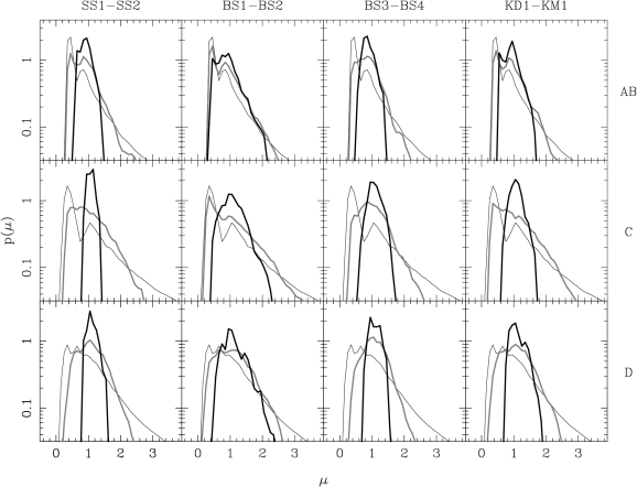
Figure 3: The magnification distributions of the various BLR models of each of the quasar images in Q2237+0305. The models run vertically, with the model name at the top of each column, while the name of each quasar image is presented down the right hand side. The thin line in each panel corresponds to the magnification distribution of a point source. The grey lines correspond to the magnification distributions for the BLR models with a radius of 1ER, whereas the black line is the magnification distribution for BLRs of radius 4ER.

Magnification maps were constructed using a ray-tracing algorithm (Kayser et al., 1986; Wambsganss et al., 1990). For each image, a square region 20 ER on a side was generated. The resolution was chosen such that one ER corresponded to 128 pixels and the number of rays traced ensured that the Poissonian error in the mean magnification was less than 0.5%.

2.2 BLR Models

To address the question of how microlensing influences the BLR it is important to determine how the region appears at particular velocities. To undertake this, the BLR models of Abajas et al. (2002) were adopted; the mathematics of these models are presented in this earlier paper and will not be reproduced here. The BLRs were constructed via a Monte Carlo approach, randomly distributing large numbers of clouds with the appropriate spatial, emissivity and velocity characteristics. By selecting in velocity, images of the source in 100 velocity slices were constructed. As per the earlier study of Abajas et al. (2002), two sizes for the BLR were considered, a smaller source with a radius of 1 ER, as well as a larger source of radius 4 ER. A summary of the eight models employed in this study is presented in Table 1; this labeling will be used through the rest of this study.

Table 1: Summary of BLR models: For each model, p denotes the radial form of the velocity field, such that $v\propto r^{\rm p}$, while $\theta$ represents the orientation of non-spherically symmetric models [see Abajas et al. (2002)].

Name	Description
SS1	Spherical Shell (p=0.5)
SS2	Spherical Shell (p=2.0)
BS1	Biconical Shell (p=0.5, $\theta=0^{o}$)
BS2	Biconical Shell (p=2.0, $\theta=0^{o}$)
BS3	Biconical Shell (p=0.5, $\theta=90^{o}$)
BS4	Biconical Shell (p=2.0, $\theta=90^{o}$)
KD1	Keplerian Disk (p=-0.5, $\theta=45^{o}$)
KM1	Modified Disk (p=-0.5, $\theta=45^{o}$)

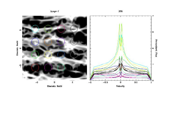
Figure 4: An example of the modification of the BLR line profile for the smaller BS2 for the microlensing model of Image C. In this panel, lighter regions denote regions of magnification, whereas darker regions correspond to regions of demagnification. In the left hand panel, the magnification map, convolved with the surface brightness distribution of the BLR, is presented. The right hand panel presents several microlensed BLR line profiles for the locations indicated by the colour-coded circles over the magnification map. The thick black line corresponds to the unmicrolensed line profile. Note that, due to the symmetric nature of the model surface brightness distribution in velocity space, the microlensed BLR line profile is symmetric in velocity.

3 Results

To calculate the influence of the gravitational microlensing magnification upon the BLR, each image of the source (as a function of velocity) was convolved with the magnification maps. For the larger BLR models, the source size becomes comparable to the scale of the magnification maps. Hence, appropriate regions are trimmed from the convolved maps to negate edge effects. For the smaller sources, this means that the central 18² ER were employed for analysis, whereas the larger sources yielded a region 12² ER. Note that for the purposes of this study, all models are oriented perpendicular to the shear field. Random orientations of the BLR models with respect to the microlensing structure is reserved to a future contribution.

3.1 Magnifications

The magnification distributions of the total flux of the BLR models, determined by convolving the velocity integrated surface brightness profile with the magnification maps, are presented in Figure 3. Note that each panel presents a pair of models, denoted at the top of each column; this is because in each pair of models the radial emission properties of the clouds are the same so that the velocity integrated surface brightness profiles are the same. This can be seen in the lowest series of panels in Figure 2. In each panel, three curves are given; the lightest is the magnification distribution of a single pixel, whereas the thicker, grey line is the distribution for the smaller BLR models. The thick black line corresponds to the magnification distribution for the larger BLR models.

As the source size increases, the width of the magnification probability distribution decreases; in comparing the single pixel source with the smaller BLR model, it is clear that the high magnification tail has been curtailed . The smaller BLR model can, however, suffer significant magnification, with the total flux in the line being boosted by a factor of 1.5-2 in most of the cases. On the face of it, this is rather surprising as the source radius of 1 ER is relatively large. It is important to remember, however, that unlike numerous previous microlensing studies, the source here is not uniform, but possesses structure on scales substantially smaller than an ER and this can be more significantly magnified.

Examining the magnification probability distributions for the larger BLR models reveals that they too can be substantially magnified, although the magnification distribution is narrower than the case of the smaller BLR sources. In most cases, the BLR can be enhanced by $\sim 50\%$. Interestingly, the $BS1$-$BS2$ pair of models are particularly broad compared to the other cases; examining Figure 2 reveals that the surface brightness distributions for these models are quite centrally concentrated compared to the other models, and this small scale structure can be substantially magnified. Again, this smaller scale structure of the BLR surface brightness distribution results in stronger magnification than a uniform source of the same radius.

This is further illustrated in Figure 4 which presents the form of the BLR emission line profile for the smaller BS2 model as microlensed by Image C in 2237. The left hand panel presents the magnification map convolved with the BS2 surface brightness distribution. The series of coloured circles over the map indicated 16 fiducial locations over the map where the form of the emission line profile were calculated. These are presented in the right hand panel, with the solid black line being the unlensed emission line profile; note that the flux in the microlensed line profiles has been divided by the mean magnification of the microlensing map so that a meaningful comparison between them and the unlensed case can be made.

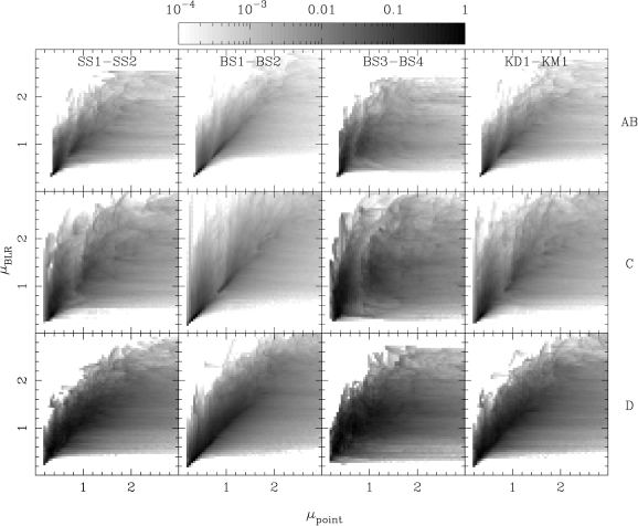
Figure 5: The correlation between the magnification of a point-like source (here one pixel) and the smaller BLR models, for simultaneous observations. Note that the relative probabilities are displayed logarithmically as denoted by the gray-scale at the top of the figure.

It is clear that there is substantial variation in not only the total emission line flux, but also in the form of the emission line profile. The red source in the lower left hand corner lies primarily in a rather uniform region of demagnification and while its emission line profile is clearly suppressed it appears to have retained its overall shape. The line profile of the dark blue source on the far left hand side, while being magnified in the wings of the line, appears to be unmagnified at velocities near zero. Examining the source profile as a function of velocity (Figure 2) it is apparent that the BS2 model is very centrally concentrated at velocities near zero, appearing more extensive at the velocity extremes. When examining the magnification map in the vicinity of the blue source it can be seen that the outer regions overlay strong magnification, whereas the central regions lie in regions of mean magnification. The opposite is true for the light green source at the top of the second column from the left. Here, the central regions of the BLR lie within a region of strong magnification, whereas the outer regions are are less affected, leading to a strong enhancement of the emission line profile at velocities near zero.

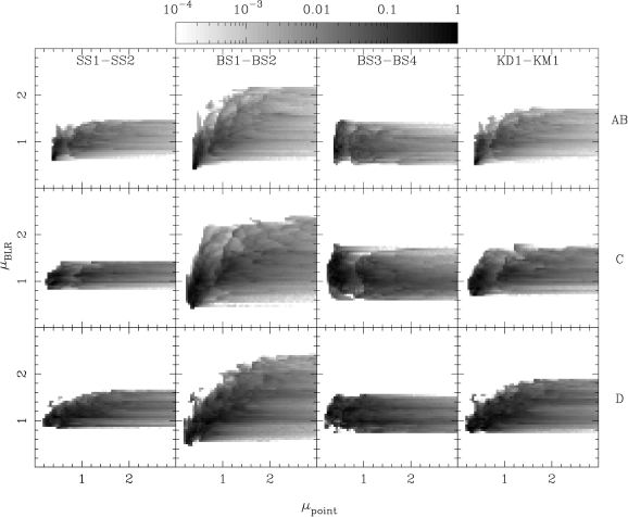
Figure 6: As for Figure 5, except for the larger BLR models.

Typically, gravitational microlensing is observed via the photometric monitoring of multiply imaged quasars (Woźniak et al., 2000; Alcalde et al., 2002) with no program of spectroscopic monitoring of any system. To observe microlensing of the BLR, therefore, it is important to know whether expected fluctuations are correlated with those of the central continuum source; this would be somewhat expected as the continuum source, which lies at the centre of the BLR, ‘sees’ similar caustic structure to the inner parts of the BLR. Figure 5 (smaller BLR source) and Figure 6 (larger BLR source) present the distributions of the magnifications of the continuum source (taken to be a single pixel in the magnification map) versus the magnification of the BLR for coincident observations. Note that the relative probability, displayed in grayscale, is presented logarithmically.

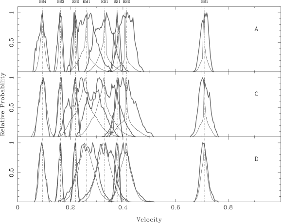
Figure 7: The variation in the centroid velocity for positive velocity half of the emission line profile for each of the models presented in this paper. The solid black line is for the smaller BLR model, where as the thicker, grey line is for the corresponding larger model. The vertical dot-dashed line indicates the location of the unlensed centroid position, with the label for each model given at the top of the line.

In examining Figures 5 and 6 it is clear that there is small scale structure in the combined probability distributions; this is due to the finite size of the magnification maps employed, with the structure due to the characteristics of the caustic networks. Overall trends, however, are apparent. Firstly, there is a general correlation between the magnification of the continuum and the BLR. For the smaller BLR source, this most apparent for the $BS1$-$BS2$ models. As discussed previously, these models present a quite compact surface brightness distribution to the caustic network and is, therefore, more similar in scale to the continuum source. In general, the magnifications are correlated for $\mu\leq 1$; this results from the fact that regions of demagnification can be extended on scales greater than an ER and hence both the BLR and continuum region can be demagnified together. However, the correlation of magnifications is weaker at $\mu>1$, showing considerable scatter for all of the models. This can be understood in terms of the clustering of the caustic network in regions of high magnification which exhibits structure on quite small scales. With this, the magnification of the continuum mirrors this small scale caustic structure, whereas the BLR is magnified by a weighted average of the larger scale caustic structure. Interestingly, for all the models, there is also a non-zero probability that while the continuum source is being strongly magnified, the over all BLR region is undergoing demagnification. The reverse of this, however, appears to be significantly rarer in most models.

The situation is very similar for the larger BLR models (Figure 6). As expected from Figure 3, the distributions of BLR magnification are somewhat narrower than the smaller BLR model. Again, no clear correlation of the continuum and BLR magnification is apparent with the continuum source undergoing significant magnification while the BLR is relatively unmagnified. It is also apparent that while there is the general correlation between the magnification of the two regions, there is still a significant range over which the continuum source can be substantially magnified while the BLR undergoes a magnification of $\sim 1$. Hence, a microlensing fluctuation observed in broadband photometric monitoring will not necessarily be an indicator of strong microlensing of the BLR. Rather than spectroscopic monitoring, however, broadband monitoring could be combined with observations obtained through a narrow band filter which covers a broad line in the quasar spectrum. With this, a plot similar to those presented in Figures 5 and 6 could be constructed and compared to simulations.

3.2 Velocity Shifts

As well as the total magnification of the emission lines, it is important to characterize the modification of the emission line profile due to differential magnification effects. This can be seen as a shift in the velocity centroid of the emission line. In undertaking this, however, it is important to note the $SS$ and $BS$ models display surface brightness structure which is symmetrical in velocity, and any gravitational lensing magnification results in identical line profile modification at positive and negative velocities, leading to a centroid shift of zero. Therefore, in the following study only the positive velocity component of the emission lines are considered for the $SS$ and $BS$ models, whereas the positive velocity and the total emission line profile are considered for the $KD1$ and $KM1$ models.

Figure 7 presents the distribution of the measured centroid of the positive velocity component of the BLR emission line for each of the models presented in this paper. The black line presents the distributions for the smaller BLR models for each lensed image, whereas the thicker, grey line represents the larger BLR models. The vertical dot-dashed line running vertically through the panels represents the unlensed location of the line centroid. Table 2 summarizes the distributions presented in Figure 7, presenting their root mean square (RMS); note that in these values are percentages of the line width at positive velocities. Several features are apparent. Firstly, the widths of the distributions are relatively insensitive to the microlensing model, with each presenting very similar forms of the distribution. Furthermore, the centroid shifts for the larger BLR models are similar or are broader than those for the smaller BLR models. This result is somewhat surprising, given that the larger BLR models undergo less microlensing magnification, a point returned to below.

Table 2 summarizes the RMS width of the distributions presented in Figure 7 as a percentage of the positive velocity line width. The width of the distribution does depend on the BLR model under consideration, with the disk models $KD1$ and $KM1$, as well as $BS3$ displaying significantly broader centroid distributions than the other models. Examining the surface brightness distributions presented in Figure 2 it is apparent that the two disk models present quite different surface brightness structures in each of the velocity slices. Hence these undergo differing degrees of lensing magnification, but as their brightness in each slice is non-negligible, this can lead to appreciable centroid shifts. Other models, such as $BS3$ and $BS4$ are luminous only in a narrow range of velocity, and magnification of this leads to only slight centroid shifts.

Figures 8 & 9 present the probability distributions of the centroid shift (presented in Figure 7) as a function of the total magnification of the smaller BLR, with the corresponding distributions for the larger BLR presented in Figure 9. These distributions are presented logarithmically on the same scale as those in Figures 5 and 6. Again, it is clear that some of the structure in these distributions is due to the limited size of the magnification maps, but some features are present. Firstly, it appears that the largest centroid shifts occur typically at lower overall magnification. In this regime, only a small range in velocity must be magnified, leading to a centroid shift but no substantial increase in the total line flux. For the total line flux to be enhanced, a substantial proportion of all velocity structure must be magnified; with this, the centroid shift would be small. Further, the distribution of the centroid shifts appears, in a number of cases, to be quite asymmetric. This again is related to the surface brightness distribution as a function of velocity.

For the asymmetric surface brightness distributions ($KD1$ & $KM1$) the line asymmetry was defined to be

$$A=100\times abs\left(\frac{f_{+}-f_{-}}{f_{+}-f_{-}}\right),$$ (1)

where $f_{+}$ is the flux in the positive velocity fraction of the emission line and $f_{-}$ is the flux in the negative velocity region. Noting that the $KD1$ and $KM1$ models are identical in either integrated positive or negative velocity, only one of these need be considered further. Figure 10 presents the probability distribution of the line asymmetry for the disk models presented in this paper, with each horizontal panel representing the results for various microlensing models. In each panel, the black line is for the smaller BLR models, whereas the thicker, grey line is for the larger BLR models. The distributions for the various models are not dissimilar, showing that substantial asymmetries in line flux (up to $\sim$20-30%) can result for the smaller BLR models when they are microlensed. Surprisingly, however, is the fact that while the magnification of the larger BLR models is typically smaller for the more extended BLR models, the substantial line asymmetries still result. This regime mirrors that earlier probed by Schneider & Wambsganss (1990) who found that, for the larger BLR models they were considering, the total magnification may be mild, but substantial asymmetric modification of the emission line profile can result.

Table 2: The widths of the centroid shift distributions presented in Figure 7

Name	Small BLR (A,C,D)	Large BLR (A,C,D)
SS1	(0.67,1.08,0.80)	(0.96,0.86,0.72)
SS2	(0.52,0.75,0.58)	(0.65,0.85,0.65)
BS1	(1.13,1.66,1.34)	(1.38,1,94,1.48)
BS2	(2.05,3.06,2.43)	(2.49,3.51,2.67)
BS3	(0.58,0.86,0.64)	(0.82,0.78,0.65)
BS4	(1.00,1.50,1.11)	(1.40,1.18,1.09)
KD1	(2.56,3.78,2.98)	(3.24,4.67,3.32)
KM1	(2.79,4.10,3.25)	(3.51,5.00,3.57)

4 Conclusions

Recent studies have reappraised the scales of structure in quasars, with the indication that the BLR, responsible for the broad emission lines seen in quasar spectra, is smaller than previously thought. This reduction in size makes the region more sensitive to the influence of gravitational microlensing. This paper has examined this influence on eight models of the BLR, considering the microlensing parameters of the multiply imaged quasar Q2237+0305, extending previous studies into the high optical depth regime.

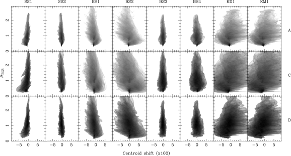
Figure 8: The centroid shift in velocity versus the total magnification of the BLR for each of the models presented in this paper. This figure considers solely the smaller BLR models. The greyscale is identical to that presented in Figure 5.

For the purpose of this study, two source sizes were adopted; a small source with a radius of 1 ER and a larger source with a radius of 4 ER. It was found that the smaller source can undergo significant magnification, with the total line flux being enhanced by a factor of 2 on occasions. At the other extreme, this smaller source can be substantially demagnified (with respect to the mean magnification) such that its total flux is reduced to 20% of the mean magnified value. As expected, the variations are less dramatic for the larger sources, with a typical demagnification to $\sim 80\%$, with magnification extremes of $1.5\times\rightarrow 2\times$. In earlier studies which considered larger BLR models, the total line flux was found to remain relatively unchanged during microlensing. If, however, the revised BLR sizes are correct, this paper has demonstrated that substantial fluctuations in the total line flux should result. This has an important consequence for studies of gravitational lensing as it implies that the relative broad line flux between images is not a measure of the relative image macromagnifications, a quantity important to gravitational lensing modelling.

Furthermore, this paper investigated the degree of modification of the form of the BLR emission line via a measurement of its centroid. The majority of models considered possess symmetric surface brightness structure in velocity space, and the overall velocity centroid of the emission line remains unchanged during microlensing. However, considering only one half of the emission line it was found that substantial modification of the emission line profile can result. Additionally, considering disk models that present asymmetric surface brightness structure as a function of velocity, it is seen that substantial centroid shifts of the entire emission line of $\sim 20\%$ can result.

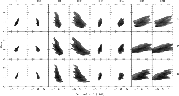
Figure 9: As for Figure 8, except for the larger BLR models.

Important differences were found in the microlensed behaviour for the models under consideration in this paper, with the degree of magnification and shift in the line centroid being dependent upon the surface brightness distribution as a function of velocity. An obvious example of this would be the detection of asymmetric modification of the overall emission line profile, indicating a surface brightness distribution which is asymmetric in velocity, such as a structure possessing rotation. While it goes beyond this current paper, these results reveal the possibility of undertaking detailed microlensing tomography of the BLR via spectroscopic monitoring of multiply imaged quasars. However, current microlensing monitoring programs focus upon obtaining broadband photometry, effectively determining the the microlensing light curves for the continuum source. Previous spectroscopic studies have revealed interesting BLR profile line differences between various images (e.g. Filippenko, 1989), although no systematic spectroscopic program has been undertaken with most studies consisting of single or double epoch observations (e.g. Lewis, Irwin, Hewett, & Foltz, 1998). To fully determine the observational implications of this study, an investigation of the temporal relationship between the microlensing of the BLR and the continuum emitting source is required, allowing the development of an optimum override strategy such that spectroscopic observations can be obtained. This is the subject of a forthcoming article.

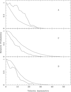
Figure 10: The asymmetry in the BLR emission line for the two disk models presented in this paper. The black line denotes the asymmetry for the smaller BAL radius models, whereas the thicker grey line represents the larger models.

5 Acknowledgments

Joachim Wambsganss is thanked for providing a copy of his microlensing raytracing code which was employed in this study and Scott Croom is thanked for helping unraveling what bright means when talking about quasars. The authors are extremely grateful to The Centre for Astrophysics and Supercomputing at Swinburne University of Technology for providing substantial computational resources available to this project, and apologize to B. Conn, J. Chapman and I. Klamer for the mondas’s screeching alarm when its cpus overheated.

References

- Abajas et al. (2002) Abajas C., Mediavilla E., Muñoz J. A., Popović L. C., Oscoz A., 2002, ApJ, 576, 640
- Alcalde et al. (2002) Alcalde, D. et al. 2002, ApJ, 572, 729
- Belle & Lewis (2000) Belle K. E., Lewis G. F., 2000, PASP, 112, 320
- Davidson & Netzer (1979) Davidson, K. & Netzer, H. 1979, Reviews of Modern Physics, 51, 715
- Filippenko (1989) Filippenko A. V., 1989, ApJ, 338, L49
- Irwin et al. (1989) Irwin, M. J., Webster, R. L., Hewett, P. C., Corrigan, R. T., Jedrzejewski, R. I. 1989, AJ, 98, 1989
- Jaroszynski, Wambsganss, & Paczynski (1992) Jaroszynski, M., Wambsganss, J., & Paczynski, B. 1992, ApJ, 396, L65
- Kaspi et al. (2000) Kaspi, S., Smith, P. S., Netzer, H., Maoz, D., Jannuzi, B. T., & Giveon, U. 2000, ApJ, 533, 631
- Kayser et al. (1986) Kayser R., Refsdal S., Stabell R., 1986, A&A, 166, 36
- Lewis & Belle (1998) Lewis G. F., Belle K. E., 1998, MNRAS, 297, 69
- Lewis, Irwin, Hewett, & Foltz (1998) Lewis, G. F., Irwin, M. J., Hewett, P. C., & Foltz, C. B. 1998, MNRAS, 295, 573
- Muñoz et al. (1998) Muñoz J. A., Falco E. E., Kochanek C. S., Lehar J., McLeod B. A., Impey C. D., Rix H.-W., Peng C. Y., 1998, Ap&SS, 263, 51
- Nemiroff (1988) Nemiroff R. J., 1988, ApJ, 335, 593
- Peterson et al. (1985) Peterson B. M., Meyers K. A., Carpriotti E. R., Foltz C. B., Wilkes B. J., Miller H. R., 1985, ApJ, 292, 164
- Rees, Netzer, & Ferland (1989) Rees, M. J., Netzer, H., & Ferland, G. J. 1989, ApJ, 347, 640
- Schmidt et al. (1998) Schmidt R., Webster R. L., Lewis G. F., 1998, MNRAS, 295, 488
- Schneider & Wambsganss (1990) Schneider P., Wambsganss J., 1990, A&A, 237, 42
- Wambsganss (1992) Wambsganss J., 1992, ApJ, 392, 424
- Wambsganss et al. (1990) Wambsganss J., Paczynski B., Katz N., 1990, ApJ, 352, 407
- Wambsganss & Paczynski (1991) Wambsganss, J. & Paczynski, B. 1991, AJ, 102, 864
- Wandel, Peterson, & Malkan (1999) Wandel, A., Peterson, B. M., & Malkan, M. A. 1999, ApJ, 526, 579
- Woźniak et al. (2000) Woźniak, P. R., Alard, C., Udalski, A., Szymański, M., Kubiak, M., Pietrzyński, G., & Zebruń, K. 2000, ApJ, 529, 88
- Wyithe & Loeb (2002) Wyithe J. S. B., Loeb A., 2002, ApJ, 577, 615
- Wyithe, Webster, Turner, & Mortlock (2000) Wyithe, J. S. B., Webster, R. L., Turner, E. L., & Mortlock, D. J. 2000, MNRAS, 315, 62
- Yonehara (1999) Yonehara, A. 1999, ApJ, 519, L31