S1296-2147 FLA ???? ? 0 2003 1 ?? J.-Ch. Hamilton CMB map-making and power spectrum estimation RubriqueHeading Sous-rubriqueSub-Heading Jean-ChristopheHAMILTON blank The Cosmic Microwave Background

CMB map-making and power spectrum estimation

CMB data analysis is in general done through two main steps : map-making of the time data streams and power spectrum extraction from the maps. The latter basically consists in the separation between the variance of the CMB and that of the noise in the map. Noise must therefore be deeply understood so that the estimation of CMB variance (the power spectrum) is unbiased. I present in this article general techniques to make maps from time streams and to extract the power spectrum from them. We will see that exact, maximum likelihood solutions are in general too slow and hard to deal with to be used in modern experiments such as Archeops and should be replaced by approximate, iterative or Monte-Carlo approaches that lead to similar precision.

 

1 Introduction

The cosmological information contained in the Cosmic Microwave Bacground (CMB) anisotropies is encoded in the angular size distribution of the anisotropies, hence in the angular power spectrum and noted $C_{\ell}$. It is of great importance to be able to compute the $C_{\ell}$ spectrum in an unbiased way. The simplest procedure to obtain the power spectrum is to first construct a map of the CMBA from the data timelines giving the measured temperature in one direction of the sky following a given scanning strategy on the sky, this is known as the map-making process ; then extract the $C_{\ell}$ from this map, this is the power spectrum extraction. Various effects usually present in the CMB data make these two operations non trivial. The major effect being related to the unavoidable presence of instrumental and photon noise. Noise in the timelines is correlated and appears as low frequency drifts that are still present in the map. A good map-making process minimizes these drifts, but in most cases, they are still present in the map. They have to be accounted for in the power spectrum estimation as the signal power spectrum is nothing but an excess variance in the map at certain angular scales compared to the variance expected from the noise. The CMBA power spectrum will therefore be unbiased only if the noise properties are known precisely.

This article presents the usual techniques that allow an unbiased determination of both the CMBA maps and power spectrum. In Sect. 2 we will describe the data model and the data statistical properties required for the techniques presented here to be valid. Sections 3 and 4 respectively deal with map-making and power spectrum estimation techniques.

2 Data model 

The initial data are time ordered information (TOI) taken along the scanning strategy pattern of the experiment. The detector measures the temperature of the sky in a given direction through an instrumental beam. This is equivalent to say that the underlying sky is convolved with this instrumental beam and that the instrument measures the temperature in a single direction of a $N_{p}$ pixellised convolved sky noted $\mathbf{T}$. The $N_{t}$ elements TOI noted $\mathbf{d}$ may therefore be modelled as:

$$\mathbf{d}=A\cdot\mathbf{T}+\mathbf{n}$$ (1)

The pointing matrix $A$ relates each time sample to the corresponding pixel in the sky. $A$ is a $N_{t}\times N_{p}$ matrix that contains a single 1 in each line as each time sample is sensitive to only one pixel is the convolved sky. The noise TOI $\mathbf{n}$ in general has a non diagonal covariance matrix $N$ given by:

$$N=\left<\mathbf{n}\cdot\mathbf{n}^{t}\right>$$ (2)

The most important property of the noise, that will be used widely later is that it has to be Gaussian and piece-wise stationary. Both assumptions are crucial as they allow major simplifications of the map-making and power spectrum estimation problems, namely Gaussianity means that all the statistical information on the noise is contained in its covariance matrix and stationarity means that all information is also contained in its Fourier power spectrum leading to major simplifications of the covariance matrix : the noise depends only on the time difference between two samples and $N$ is therefore a Toeplitz matrix $N_{ij}=N_{\left|i-j\right|}$ completely defined by its first line and is very close to be circulant. Such a matrix is diagonal in Fourier space. Its first line is given by the autocorrelation function of the noise, that is the inverse Fourier transform of its Fourier power spectrum ($\star$ is the convolution operator):

$$N_{i0}=\left<\mathbf{n}\star\mathbf{n}\right>\equiv\left<{\cal{F}}^{-1}\left[\left|{\cal{F}}(\mathbf{n})\right|^{2}\right]\right>$$ (3)

3 Map-making techniques

The map-making problem is that of finding the best estimate $\hat{\mathbf{T}}$ of $\mathbf{T}$ from Eq. 1 given $\mathbf{d}$ and $A$. The noise $\mathbf{n}$ is of course unknown. We will address the two main approaches to this problem, the first being the simplest one and the second one being the optimal one. An excellent detailed review on map-making techniques for the experts is [Stompor,  2002].

3.1 Simplest map-making : coaddition

The simplest map-making that one can think about is to neglect the effects of the correlation of the noise. One can just average the data falling into each pixel without weighting them. This procedure is optimal (it maximises the likelihood) if the noise in each data sample is independant, that is, if the noise is white. In a matrix notation, this simple map-making can be written:

$$\hat{\mathbf{T}}=\left[A^{t}\cdot A\right]^{-1}\cdot A^{t}\cdot\mathbf{d}$$ (4)

where the operator $A^{t}$ just projects the data into the correct pixel and $\left[A^{t}\cdot A\right]$ counts the sample falling into each pixel. This simple map-making has the great advantage of the simplicity. It is fast ($\propto N_{t}$) and robust.

However, in the case of realistic correlated noise, the low frequency drifts in the timelines induce stripes in the maps along the scans of the experiment. These stripes are often much larger than the CMBA signal that is searched for and therefore should be avoided. Various destriping techniques have been proposed to avoid these stripes. A method exploiting the redundancies of the Planck mission scanning strategy has been proposed by [Delabrouille,  1998] and extended to polarisation by [Revenu et al., 2000]. This kind of method aims at suppressing the low frequency signal by requiring that all measurements done in the same direction at different instant coincide to a same temperature signal. Another method has recently been proposed for the Archeops data analysis and estimates the low frequency drifts by minimizing the cross-scan variations in the map due to the drifts [Bourrachot et al., 2003]. The simplest method for removing the low frequency drifts before applying simple map-making is certainly to filter the timelines so that the resulting timeline has almost white noise. The filtering can consist in prewhitening the noise or directly setting to zero contaminated frequencies. The computing time (CPU) scaling of the filtering + coaddition process is modest and dominated by filtering ($\propto N_{t}\log N_{t}$). This method however removes also part of the signal on the sky and induces ringing around bright sources which has to be accounted for in later processes.

3.2 Optimal map-making

The most general solution to the map-making problem is obtained by maximizing the likelihood of the data given a noise model [Wright, 1996, Tegmark, 1997]. As the noise is Gaussian, its probability distribution is given by the $N_{t}$ dimensionnal Gaussian:

$$P(\mathbf{n})=\frac{1}{\left|(2\pi)^{N_{t}}N\right|^{1/2}}\exp\left[-\frac{1}{2}\mathbf{n}^{t}\cdot N^{-1}\cdot\mathbf{n}\right]$$ (5)

Assuming no prior on the sky temperature, one gets from Eq. 1 the probability of the sky given the data:

$$P(\mathbf{T}|\mathbf{d})\propto P(\mathbf{d}|\mathbf{T})\propto\frac{1}{\left|(2\pi)^{N_{t}}N\right|^{1/2}}\exp\left[-\frac{1}{2}\left(\mathbf{d}-A\cdot\mathbf{T}\right)^{t}\cdot N^{-1}\cdot\left(\mathbf{d}-A\cdot\mathbf{T}\right)\right]$$ (6)

Maximizing this probability with respect to the map leads to solving the linear equation:

$$A^{t}\cdot N^{-1}\cdot A\cdot\mathbf{T}=A^{t}\cdot N^{-1}\cdot\mathbf{d}$$ (7)

with solution:

$$\hat{\mathbf{T}}=\left(A^{t}\cdot N^{-1}\cdot A\right)^{-1}\cdot A^{t}\cdot N^{-1}\cdot\mathbf{d}$$ (8)

One therefore just has to apply this linear operator to the data timeline to get the best estimator of $\mathbf{T}$, note that $\hat{\mathbf{T}}$ is also the minimum variance estimate of the map. The covariance matrix of the map is:

$${\cal N}=\left(A^{t}\cdot N^{-1}\cdot A\right)^{-1}$$ (9)

Problems arise when trying to implement this simple procedure, the timeline data and the maps are in general very large : the typical dimensions of the problem are $N_{t}\simeq 6\times 10^{7}$ and $N_{p}\simeq 10^{5}$ for Archeops.

The maximum likelihood solution requires both $N^{-1}$ and $\left(A^{t}\cdot N^{-1}\cdot A\right)^{-1}$ which are not easy to determine. Two approaches can be used at this point: one can try to make a brute force inversion of the problem, relying on huge parallel computers or one can try to iteratively approach the solution, hoping that convergence can be reached within reasonnable time.

3.3 Brute force inversion

The brute force optimal map-making parallel implementation is freely available as the MADCAP [Borrill, 1999] package. It is a general software designed to produce an optimal map for any experiment by solving directly Eq. 7. The use of this package requires the access to large parallel computers.

The only assumption that is done in MADCAP map-making is that the inverse time-time noise covariance matrix can be obtained directly without inversion from the noise Fourier power spectrum:

$$N^{-1}_{i0}\simeq\left<{\cal{F}}^{-1}\left[\frac{1}{\left|{\cal{F}}(\mathbf{n})\right|^{2}}\right]\right>$$ (10)

This assumption is not perfectly correct on the edges of the matrix but leads to a good estimate of the inverse time covariance matrix for the sizes we deal with. This allows this step to scale as $N_{t}\log N_{t}$ operations rather than the $N_{t}^{2}$ required by a Toeplitz matrix inversion. In most cases, the time correlation $N_{\tau}$ length is less than the whole timestream $N_{t}$ so that $N$ is band-diagonal. For Archeops, we have $N_{\tau}\simeq 10^{4}$.

The next step is to compute the inverse pixel noise covariance matrix ${\cal N}^{-1}=\left(A^{t}\cdot N^{-1}\cdot A\right)$ and the noise weighted map $A^{t}\cdot N^{-1}\cdot\mathbf{d}$, both operations scale as $N_{t}\times N_{\tau}$ when exploiting the structure of $A$ and $N$. The last step is to invert ${\cal N}^{-1}$ and multiply it by $A^{t}\cdot N^{-1}\cdot\mathbf{d}$ to get the optimal map. Unfortunately, ${\cal N}^{-1}$ has no particular structure that can be exploited and this last step scales as a usual matrix inversion $\propto N_{p}^{3}$ and largely dominates the CPU required by MADCAP for the usual large datasets (eg. Archeops).

We can remark here that MADCAP provides the map covariance matrix ${\cal N}$ for free as a byproduct. This matrix is crucial for estimating the power spectrum as will be seen in section 4.

3.4 Iterative solutions

The other possibility is to solve Eq. 7 through an iterative process such as the Jacobi iterator, or more efficiently a conjugate-gradient [Press et al., 1988]. Both converge to the maximum likelihood solution.

The use of the Jacobi iterator for solving for the maximum likelihood map in CMB analysis was first proposed by [Prunet et al., 2000]. The basic algorithm is the following. We have to solve the following linear system (see Eq. 7):

$$\Gamma\cdot\mathbf{x}=\mathbf{y}$$ (11)

The Jacobi iterator starts with an approximation $\Lambda_{0}$ of $\Gamma^{-1}$ and iterates to improve the residuals $R$:

$$\Lambda_{0}\cdot\Gamma=I-R$$ (12)

In order to converge, the algorithm requires the first approximation to be good enough so that the eigenvalues of $R$ are all smaller than 1 (a good estimate in general is $\Lambda_{0}=\left[\mathrm{diag}\Gamma\right]^{-1}$). We can therefore expand:

$$\Gamma^{-1}=\left(I-R\right)^{-1}\cdot\Lambda_{0}=\left(I+R+R^{2}+\cdots\right)\cdot\Lambda_{0}$$ (13)

Lets us define $\Lambda_{n}=\left(I+R+R^{2}+\cdots+R^{n}\right)\cdot\Lambda_{0}$ so that $\Gamma^{-1}=\lim_{n\rightarrow\infty}\Lambda_{n}$. We have the relationship $\Lambda_{j+1}=\Lambda_{0}+R\cdot\Lambda_{j}$. If we define $\mathbf{x}_{j}=\Lambda_{j}\cdot\mathbf{y}$, it is straightforward to show that:

$$\mathbf{x}_{j+1}-\mathbf{x}_{j}=\Lambda_{0}\cdot\left(\mathbf{y}-\Gamma\cdot\mathbf{x}_{j}\right)$$ (14)

which defines the Jacobi iterator. When going back to the usual CMB notation for maps and timelines, one gets:

$$\mathbf{T}_{j+1}-\mathbf{T}_{j}=\left[\mathrm{diag}\left(A^{t}\cdot N^{-1}\cdot A\right)\right]^{-1}\cdot A^{t}\cdot N^{-1}\cdot\left(\mathbf{d}-A\cdot\mathbf{T}_{j}\right)$$ (15)

which looks rather complicated but is in fact very simple to implement: the operation $A\cdot\mathbf{T}_{j}$ just consists in reading the map at iteration $j$ with the scanning strategy ($\propto N_{t}$), and the matrix $\mathrm{diag}\left(A^{t}\cdot N^{-1}\cdot A\right)$ is just the white noise level variance divided by the number of hits in each pixel. It is diagonal and therefore does not require proper inversion. The only tricky part here is the multiplication $N^{-1}\cdot\left(\mathbf{d}-A\cdot\mathbf{T}_{j}\right)$ given the fact that $N^{-1}$ is unknown. As the noise is stationary, $N$ is Toeplitz and circulant, the multiplication by $N^{-1}$ can be done in Fourier space directly through:

$$N^{-1}\cdot\mathbf{x}\simeq{\cal F}^{-1}\left[\frac{{\cal F}(\mathbf{x})}{\left|{\cal F}(\mathbf{x})\right|^{2}}\right]$$ (16)

which requires $N_{t}\log N_{t}$ operations. Finally, each iteration is largely dominated by the latter so that the final CPU time scales like $N_{it}\times N_{t}\log N_{t}$ where $N_{it}$ is the number of iterations.

Unfortunately the convergence of such an iterator is very slow and makes it rather unefficient as it is. A significant improvement was proposed by [Doré et al., 2001] in the publicly available software MAPCUMBA. They noted that the convergence was actually very fast on small scales (compared to the pixel) but that the larger scales were converging slowly. They proposed a multigrid method where the pixel size changes at each iteration so that the global convergence is greatly accelerated (see Fig. 7 of [Doré et al., 2001]), making this iterative map-making really efficient. A conjugate gradient solver instead of the Jacobi iterator is implemented in the software Mirage [Yvon et al., in prep.] and accelerates again the convergence significantly. A new version of MAPCUMBA also uses a conjugate gradient solver, as well as MADmap [Cantalupo, 2002].

If obtaining an optimal map is now quite an easy task using an iterative implementation (the presence of strong sources, such as the galactic signal however complicates this simple picture), they do not provide the map noise covariance matrix ${\cal N}=\left(A^{t}\cdot N^{-1}\cdot A\right)^{-1}$ which is of great importance when computing the CMB power spectrum in the map in order to be able to make the difference between noise fluctuations and real signal fluctuations. The only way to obtain this covariance matrix using these iterative methods is through large Monte-Carlo simulation that would reduce the advantage of iterative map-making compared to brute-force map-making.

3.5 map-making comparisons

The precision of the MADCAP, MAPCUMBA and Mirage implementations are shown in Fig 1 with the same CMB and noise simulation based on Archeops realistic conditions. The three resulting maps were kindly provided by [Filliatre, 2002]. The six maps on the left are respectively from top left to bottom right : initial CMB fluctuation, coaddition of the timeline without filtering, coaddition of the timeline with white noise only (ie the true optimal map that has to be reconstructed), MADCAP residual map (difference between MADCAP reconstructed map and the white noise map), MAPCUMBA residual map and Mirage residual map. All maps are shown with the same color scale. The first remark that can be done is that the stripes are indeed a real problem and that straight coaddition is not to be performed. The three different optimal map-making codes give very similar results, especially MADCAP and MAPCUMBA. In all cases, as can be also seen in the right panel of Fig. 1, the residuals are much smaller than the CMB fluctuations that are searched for. The three map-making implementation can therefore be considered are unbiased.

Finally one can summarize the comparison as following, iterative and brute-force optimal map-making give very similar results as far the optimal map is concerned. The brute force inversion provides the map noise covariance matrix for free which is a major point as will be seen in next section. The computer requirements are however much larger than for iterative map-making. The latter should therefore be used when the power spectrum estimation can be carried out without the knowledge of the map noise covariance matrix, in general using a Monte-Carlo technique (see next section). In this case, one should seriously consider the filtering + coaddition map-making that is by far the fastest but removes part of the signal. This is however accounted for (see section 4.2) also using a Monte-Carlo technique.

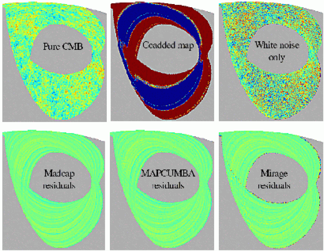
Figure 1: The six maps on the right show a comparison of results from different map-making implementations on the same simulation (typical of Archeops data). All maps are in Healpix pixellisation [Gorski et al. 1998] and have the same color scale ranging from -500 $\mu\mathrm{K}$ to 500 $\mu\mathrm{K}$ from dark blue to dark red, green corresponds to zero. The histograms of the residuals is shown on the right and is more than three times smaller than the actual CMB fluctuation.

4 Power spectrum estimation techniques

We know want to compute the power spectrum $C_{\ell}$ of the map $\mathbf{T}$ whose noise covariance matrix ${\cal N}$ might be known or not depending on the method that was used before to produce the map. The map is composed of noise and signal (from now on $\mathbf{n}$ is the noise on the map pixels):

$$\mathbf{T}=\mathbf{s}+\mathbf{n}$$ (17)

The signal in pixel $p$ can be expanded on the $Y_{\ell m}\left(\theta_{p},\phi_{p}\right)$ spherical harmonics basis :

$$s_{p}=\sum_{\ell=0}^{\infty}\sum_{m=-\ell}^{\ell}a_{\ell m}B_{\ell}Y_{\ell m}\left(\theta_{p},\phi_{p}\right)$$ (18)

where $B_{\ell}$ stands for the beam. If the CMBA are Gaussian, the variance of the $a_{\ell m}$, called the angular power spectrum and denoted $C_{\ell}$ contains all the cosmological information :

$$\left<a_{\ell m}a_{\ell^{\prime}m^{\prime}}^{\star}\right>=C_{\ell}\delta_{\ell\ell^{\prime}}\delta_{mm^{\prime}}$$ (19)

The map covariance matrix (assuming no correlation between signal and noise) is:

$$M = \left<\mathbf{T}\cdot\mathbf{T}^{t}\right>=\left<\mathbf{s}\cdot\mathbf{s}^{t}\right>+\left<\mathbf{n}\cdot\mathbf{n}^{t}\right>$$ (20)

$$= S+N$$ (21)

and the signal part is related to the $C_{\ell}$:

$$S_{pp^{\prime}}=\left<s_{p}s_{p^{\prime}}\right>=\sum_{\ell}\frac{2\ell+1}{4\pi}C_{\ell}B_{\ell}^{2}P_{\ell}(\chi_{pp^{\prime}})$$ (22)

where $\chi_{pp^{\prime}}=\cos\left(\mathbf{u}_{p}\cdot\mathbf{u}_{p^{\prime}}\right)$, $\mathbf{u}_{p}$ being the unit vector towards pixel $p$ and $P_{\ell}$ are the Legendre polynomials.

One therefore has a direct relation between the map and noise covariance matrices and the angular power spectrum:

$$M=N+\sum_{\ell}\frac{2\ell+1}{4\pi}C_{\ell}B_{\ell}^{2}P_{\ell}(\chi_{pp^{\prime}})$$ (23)

The power spectrum estimation consists in estimating $C_{\ell}$ from $\mathbf{T}$ and $N$ (that can be unknown) using this relation.

4.1 Maximum likelihood solution

Full details concerning this can be found in [Bond, Jaffe and Knox, 1998, Tegmark, 1997]. As for the map-making problem, the maximum likelihood solution proceeds by writing the probability for the map given its covariance matrix assuming Gaussian statistics:

$$P(C_{\ell}|\mathbf{T})\propto P(\mathbf{T}|C_{\ell})=\left(2\pi\right)^{-N_{p}/2}\exp\left[-\frac{1}{2}\left[\left(\mathbf{T}^{t}\cdot M^{-1}\cdot\mathbf{T}\right)+\mathrm{Tr}\left(\ln M\right)\right]\right]$$ (24)

and we therefore want to maximize the likelihood function through $\frac{\partial L}{\partial C_{\ell}}=0$:

$$L(C_{\ell})=-\frac{1}{2}\left[\left(\mathbf{T}^{t}\cdot M^{-1}\cdot\mathbf{T}\right)+\mathrm{Tr}\left(\ln M\right)\right]$$ (25)

Tedious calculations lead to the solution:

$$C_{\ell}=\sum_{\ell^{\prime}}F^{-1}_{\ell\ell^{\prime}}\times\mathrm{Tr}\left[\left(\mathbf{T}\cdot\mathbf{T}^{t}-N\right)\cdot M^{-1}\cdot\frac{\partial S}{\partial C_{\ell}}\cdot M^{-1}\right]$$ (26)

where $F$ is the Fisher matrix:

$$F_{\ell\ell^{\prime}}=\mathrm{Tr}\left[\frac{\partial S}{\partial C_{\ell}}\cdot M^{-1}\cdot\frac{\partial S}{\partial C_{\ell^{\prime}}}\cdot M^{-1}\right]$$ (27)

Eq. (26) let $C_{\ell}$ appear in both sides (in $M$) in an uncomfortable way and therefore cannot be solved simply. The method usually used [Bond, Jaffe and Knox, 1998, Borrill, 1999] is the Newton-Raphson iterative scheme: One starts from an initial guess for the binned power spectrum $\mathbf{C}^{(0)}$ and iterates until convergence following:

$$\mathbf{C}^{(i+1)}=\mathbf{C}^{(i)}+\delta\mathbf{C}$$ (28)

with:

$$\delta\mathbf{C}=-\left[\left.\frac{\partial^{2}L}{\partial\mathbf{C}^{2}}\right|_{\mathbf{C}=\mathbf{C}_{i}}\right]^{-1}\cdot\left.\frac{\partial L}{\partial\mathbf{C}}\right|_{\mathbf{C}=\mathbf{C}_{i}}$$ (29)

the likelihood $L$ being that of Eq. 25. Convergence is usually reached after a few iterations. The explicit form of the derivatives of Eq. 29 is:

$$\frac{\partial L}{\partial C_{b}} = \frac{1}{2}\left(\mathbf{m}^{T}\cdot M^{-1}\cdot\frac{\partial S}{\partial C_{b}}\cdot M^{-1}\cdot\mathbf{m}-\mathrm{Tr}\left[M^{-1}\cdot\frac{\partial S}{\partial C_{b}}\right]\right)$$ (30)

$$\frac{\partial^{2}L}{\partial C_{b}\partial C_{b^{\prime}}} = -\mathbf{m}^{T}\cdot M^{-1}\cdot\frac{\partial S}{\partial C_{b}}\cdot M^{-1}\cdot\frac{\partial S}{\partial C_{b^{\prime}}}\cdot M^{-1}\cdot\mathbf{m}+\frac{1}{2}\mathrm{Tr}\left[M^{-1}\cdot\frac{\partial S}{\partial C_{b}}\cdot M^{-1}\cdot\frac{\partial S}{\partial C_{b^{\prime}}}\right]$$ (31)

where the index $b$ denotes the bin number.

Each iteration will then require a large number of large matrix operations forcing such an algorithm to be implemented on large memory parallel supercomputers. MADCAP [Borrill, 1999] is the common implementation of this algorithm and scales as $2(N_{b}+\frac{2}{3})N_{p}^{3}$ operations per iteration. The CPU/RAM/Disk problem is therefore even cruder for the power spectrum than for the map-making. This algorithm leads to the optimal solution accounting correctly for the noise covariance matrix and additionnaly provides the likelihood shape for each bin through the various iterations allowing to a direct estimate of the error bars.

4.2 Frequentist approaches

An alternative approach to power spectrum estimation is to compute the so called pseudo power spectrum (harmonic transform of the map, noted $\tilde{C_{\ell}}$) and to correct it so that it becomes a real power spectrum. This approaches have been proposed and developped in [Hivon et al., 2001, Szapudi et al. 2001]. The harmonic transform of the map differs from the true $C_{\ell}$ in various ways (we follow the notations from [Hivon et al., 2001]): The observed sky is convolved by the beam and by the transfer function of the experiment so that the observed power spectrum is $B_{\ell}^{2}F_{\ell}C_{\ell}$, where $B_{\ell}$ characterizes the beam shape in harmonic space and $F_{\ell}$ the filtering done to the data by the analysis process (that may also include electronic filtering by the instrument itself). The observed sky is in general incomplete (at least because of a Galactic cut) leading to the fact that the $C_{\ell}$ measured are not independant as they are convolved in harmonic space by the window-function [White and Srednicki 1995]. We therefore have access to $\sum_{\ell^{\prime}}M_{\ell\ell^{\prime}}B_{\ell^{\prime}}^{2}F_{\ell^{\prime}}C_{\ell^{\prime}}$ where $M_{\ell\ell^{\prime}}$ is the mode mixing matrix. Finally, the noise in the timelines projects on the sky and adds its contribution $\tilde{N}_{\ell}$ to the sky angular power spectrum. At the end, the map angular power spectrum, the pseudo-$C_{\ell}$ is related to the true $C_{\ell}$ via:

$$\tilde{C}_{\ell}=\sum_{\ell^{\prime}}M_{\ell\ell^{\prime}}B_{\ell^{\prime}}^{2}F_{\ell^{\prime}}C_{\ell^{\prime}}+\tilde{N}_{\ell}$$ (32)

The frequentist methods propose to invert Eq. 32 making an extensive use of Monte-Carlo simulations (details can be found in [Hivon et al., 2001]):

• the pseudo power spectrum of the map $\tilde{C_{\ell}}$ is computed by transforming the map into spherical harmonics (generally using Healpix pixellisation and the anafast procedure available in the Healpix package [Gorski et al. 1998]).

• The mode mixing matrix is computed analytically through:

  $$M_{\ell_{1}\ell_{2}}=\frac{2\ell_{2}+1}{4\pi}\sum_{\ell_{3}}\left(2\ell_{3}+1\right){\mathcal{W}}_{\ell_{3}}\left(\begin{array}[]{ccc}\ell_{1}&\ell_{2}&\ell_{3}\\ 0&0&0\end{array}\right)$$ (33)

  where ${\mathcal{W}}_{\ell}$ is the power spectrum of the window of the experiment (in the simplest case 1 for the observed pixels and 0 elsewhere, but more complex weighting schemes may be used, as in Archeops [Benoît et al., 2003] or WMAP [Hinshaw et al., 2003]). In the SpICE approach [Szapudi et al. 2001], the $M_{\ell\ell^{\prime}}$ inversion in harmonic space is replaced by a division in angular space which is mathematically equivalent.

• The beam transfer function is computed from a Gaussian approximation or the legendre transform of the beam maps or a more complex modelling if the beams are asymetric, such as in [Tristram et al., in prep].

• The filtering transfer function is computed using a signal only Monte-Carlo simulation (it should include the pre-processing applied to the time streams). Fake CMB sky are passed through the instrumental and analysis process producing maps and pseudo power spectra. The transfer function is basically computed as the ratio of the input model to the recovered ensemble average. An important point at this step is to check that the transfer function is independent of the model assumed for the simulation. Let’s also remark that using a transfer function that depends only on $\ell$ is a bit daring as the filtering is done in the scan direction which, in general corresponds to a particular direction on the sky. This approximation however seems to work well and has been successfully applied to Boomerang [Netterfield et al., 2002] and Archeops [Benoît et al., 2003]).

• The noise power spectrum is computed from noise only simulations passing again through the instrumental and analysis process to produce noise only maps and pseudo power spectra. The noise power spectrum is estimated from the ensemble average of the various realisations.

• Error bars are computed in a frequentist way by producing signal+noise simulations and analysing them as the real data. This allows to reconstruct the full likelihood shape for each power spectrum bin and the bin-bin covariance matrix.

Such an approach based on simulations has the advantage of being fast: each realisation basically scales as $\propto N_{t}\log N_{t}$ for the noise simulation and map-making (if filtering + coaddition is used) and $\propto N_{p}^{3/2}$ for the CMB sky simulation and pseudo power spectrum computation. An important advantage of such a method is the possibility to include in the simulation systematic effects (beam, pointing, atmosphere, …) that would not be easily accountable for in a maximum likelihood approach.

4.3 Cross-power spectra

When several photometric channels are available from the experimental setup, it is possible to compute cross-power spectra between the channel rather than power spectra of individual channel or of the average of all channels. This has the advantage of suppressing the noise power spectrum (but not its variance of course) that is not correlated between channels and leaving the sky signal unchanged. The cross-power spectrum of channels $i$ and $j$ is defined as:

$$C_{\ell}^{i,j}=\frac{1}{2\ell+1}\sum_{m=-\ell}^{\ell}a_{\ell m}^{i}a_{\ell m}^{j\star}$$ (34)

The cross-power spectrum method can easily be associated with the frequentist approach simplifying significantly it implementation as one the most difficult part, the noise estimation, is now less crucial as noise disapears and cannot bias the power spectrum estimation. This has been successfuly applied in the WMAP analysis [Hinshaw et al., 2003].

4.4 Which power spectrum estimator should be used ?

The maximum likelihood approach is undoubtly the best method to use if possible, but its CPU/RAM/Disk requirements are such that in practice, with modern experiments, it is very difficult to implement. It should however be considered to check the results on data subsets small enough to make it possible. The frequentist approaches are much faster and provide comparable precision in terms of error bars and permit to account for systematic effects in a simple manner. The tricky part is however to estimate the noise statistical properties precisely enough. The same difficulty exists however in the maximum likelihood approach where the noise covariance matrix has to be known precisely. It is generally directly computed in the map-making process from the time correlation function, thus displacing the difficulty elsewhere. In any case, the noise model has to be unbiased as the final power spectrum is essentially the subtraction between the pseudo power spectrum of the map and the noise power spectrum. Estimating the noise properties is a complex problem mainly due to signal contamination and pixellisation effects. A general method for estimating the noise in CMB experiment is proposed in [Amblard & Hamilton, 2003] and was successfuly applied for the Archeops analysis [Benoît et al., 2003]. When multiple channels are available, the frequentist approach applied on cross-power spectra is certainly the simplest and most powerful power spectrum estimation technique available today as it reduces the importance of the difficult noise estimation process. We can also mention the hierarchical decomposition [doré et al., 2001] that achieves an exact power spectrum estimation to submaps at various resolutions, and then optimally combine them.

5 Conslusions

We have shown techniques designed to make maps from CMB data and to extract power spectra from them. In both cases, the brute force, maximum likelihood approach is the most correct, but generally hard to implement in practice. Alternative approaches, iterative or relying on Monte-Carlo simulations provide similar precision with smaller computer requirements. In all cases, a lot of work has to be done before : first by designing the instrument correctly and afterwards by cleaning the data, flagging bad samples and ending up with a dataset that match the minimum requirement of all the methods described in this review : stationarity and Gaussianity.

The Author wants to thank the Archeops collaboration for its stimulating atmosphere, A. Amblard and P. Filliatre for reading carefully the manuscript and providing useful inputs.

References

- [Stompor, 2002] R. Stompor et al., Phys. Rev. D, 65 (2002), 022003.
- [Delabrouille, 1998] J. Delabrouille, A&AS, 127 (1998), 555-567.
- [Revenu et al., 2000] B. Revenu et al., A&AS, 142 (2000), 499-509.
- [Bourrachot et al., 2003] A. Bourrachot et al., in preparation.
- [Wright, 1996] E.L.. Wright, astro-ph/9612006.
- [Tegmark, 1997] M. Tegmark, Phys. Rev. D, 56 (1997), 4514.
- [Borrill, 1999] J. Borrill, Proc. of the 5th European SGI/Cray MPP Workshop (1999), astro-ph/991389.
- [Press et al., 1988] W.H. Press et al., Numerical recipes in C (1988), Cambridge University Press.
- [Prunet et al., 2000] S. Prunet et al., astro-ph/0006052.
- [Doré et al., 2001] O. Doré et al., A&A, 374 (2001), 358D.
- [Yvon et al., in prep.] D. Yvon et al., in preparation.
- [Cantalupo, 2002] C. Cantalupo http://www.nersc.gov/ cmc/MADmap/doc/index.html.
- [Filliatre, 2002] P. Filliatre, PHD thesis, Universitè Joseph Fourier, Grenoble, France (2002)
- [Gorski et al. 1998] K.M. Gorski et al., astro-ph/9812350, http://www.tac.dk/~healpix/.
- [Bond, Jaffe and Knox, 1998] J.R. Bond, A.H. Jaffe and L. Knox, Phys. Rev. D57, 2117 (1998).
- [Tegmark, 1997] M. Tegmark, Phys. Rev. D55, 5895 (1997).
- [Hivon et al., 2001] E. Hivon et al., astro-ph/0105302.
- [Szapudi et al. 2001] I. Szapudi et al., astro-ph/0107383.
- [White and Srednicki 1995] M. White and M. Srednicki, ApJ, 443, 6 (1995).
- [Benoît et al., 2003] A. Benoît et al., A&A, 399 (2003), 19L.
- [Hinshaw et al., 2003] G. Hinshaw et al., astro-ph/0302217, submitted to ApJ.
- [Tristram et al., in prep] M. Tristram et al., in preparation.
- [Netterfield et al., 2002] C.B. Netterfield et al., ApJ, 571 (2002), 604.
- [Amblard & Hamilton, 2003] A. Amblard & J.-Ch. Hamilton, submitted to A&A.
- [doré et al., 2001] O. Doré, L. Knox and A. Peel, Phys.Rev. D64 (2001) 083001.