FLY. A parallel tree N-body code for cosmological simulations. Reference Guide

Abstract

FLY is a parallel treecode which makes heavy use of the one-sided communication paradigm to handle the management of the tree structure. In its public version the code implements the equations for cosmological evolution, and can be run for different cosmological models.
This reference guide describes the actual implementation of the algorithms of the public version of FLY, and suggests how to modify them to implement other types of equations (for instance the Newtonian ones).

, and

PROGRAM SUMMARY

Title of Program: FLY

Catalogue Identifier:

Distribution Format:

Computer for which the program is designed and others on which it has been tested: Cray T3E, Sgi Origin 3000, IBM SP

Operating systems or monitors under which the program has been tested: Unicos 2.0.5.40 , Irix 6.5.14, Aix 4.3.3

Programming language used: Fortran 90, C

Memory required to execute with typical data: about 100 Mwords with 2 million-particles

Number of bits in a word: 32

Number of processors used: parallel program. The user can select the number of processors $\geq 1$

Has the code been vectorised or parallelized?: parallelized

Number of bytes in distributed program, including test data, etc: 110 Mbytes

Distribution format: tar gzip file

Keywords: Parallel tree N-body code for cosmological simulations

Nature of physical problem: FLY  is a parallel collisionless N-body code for the calculation of the gravitational force

Method of solution: It is based on the hierarchical oct-tree domain decomposition introduced by Barnes and Hut (1986)

Restrictions on the complexity of the program: The program uses the leapfrog integrator schema, but could be changed by the user

Typical running time : 50 seconds for each time-step, running a 2-million-particles simulation on an Sgi Origin 3800 system with 8 processors having 512 Mbytes Ram for each processor

Unusual features of the program : FLY  uses the one-side communications libraries: the shmem library on the Cray T3E system and Sgi Origin system, and the lapi library on IBM SP system

References : U. Becciani, V. Antonuccio Comp. Phys. Com. 136 (2001) 54

LONG WRITE-UP

1 Introduction

FLY  is a parallel collisionless N-body code which relies on the hierarchical oct-tree domain decomposition introduced in 1986Natur.324..446B for the calculation of the gravitational force. Although there exist different publicly available parallel treecodes, FLY  differs from them because it heavily relies on two parallel programming concepts: shared memory and one-sided communications. Both of these concepts are implemented in the SHMEM library of the UNICOS operating system on the CRAY T3E and Sgi Origin computing systems.
FLY  is the result of the development of a preliminary software called WD99. This code was developed in the period 1996-2000 using several platforms. The first release was developed with the CRAFT programming environment embedded the Cray T3D. The porting of the code on the Cray T3E system, where the CRAFT was no more available, was performed in 1998 using the shmem library, that was the only one-side communication system available. The performances of the shmem library, in terms of scalability and latency time are very good, being this library designed for the hardware architecture of the Cray T3E and of the Sgi Origin systems. On systems like the IBM SP where these libraries are not available FLY  has been modified to use the local libraries.
The MPI-2 library was made available with good declared performances for IBM SP System only recently. This library probably will be adopted in the next FLY  version, to increase the code portability.
A more detailed treatment of the parallel computing techniques which have been adopted and of the resulting performances on different systems can be found elsewhere.
Being an open source project, FLY  can and must be modified to suit the particular needs of individual users. In order to ease this, we will describe some features concerning the integration of the equations of motion (section 2), the generation of initial conditions, the structure of the checkpoint and the output files. In section 5 we will also describe the structure of some parameter files needed to run a simulation. More detailed information concerning the preparation of these parameter files, the compilation and running of the code can be found in the FLY  User Guide flyug .

2 Equations of motion.

The actual form of the discretized equations of motion is implemented in the subroutines upd_pos and upd_vel; if the user needs to identify some special parameters which are used in these subroutines, he may want to define them in initpars. In the publicly distributed version of FLY  , we have implemented a set of cosmological equations of motion, solving the standard particle equations of motion for a Friedmann cosmology. In the following, we will present these equations and their discrete implementation.
The Friedmann-Robertson-Walker metric is characterized by an expansion factor $a(t)$, where $t$ is the conformal time. Let $\boldsymbol{x}_{i}(t)$ be the comoving coordinate of the $i$-th particle and $m_{i}$ its mass, then the equations of motion are given by:

$$\dot{\boldsymbol{x}_{i}}=\boldsymbol{v}_{i}$$ (1)

$$\dot{\boldsymbol{v}_{i}}+2\frac{\dot{a}}{a}\boldsymbol{v}_{i}=-\frac{G}{a^{3}}\sum_{j\neq i}\frac{m_{j}(\boldsymbol{x}_{i}-\boldsymbol{x}_{j})}{\mid\boldsymbol{x}_{i}-\boldsymbol{x}_{j}\mid^{3}}+\boldsymbol{F}_{Ewald}(\boldsymbol{x})$$ (2)

Here and in the following a dot denotes derivation w.r.t. the conformal time variable $t$, $G$ is the gravitational constant and the last term, $\boldsymbol{F}_{Ewald}(\boldsymbol{x})$, is the Ewald correction, which takes into account the contribution to the force from the infinite replicas of the simulation box over the spatial directions. We also define the Hubble constant: $H(t)=\dot{a}/a$.
It is more convenient to introduce a set of dimensionless spatial, temporal and mass variables:

$$\boldsymbol{x}_{i}^{\prime}=L_{0}\boldsymbol{x}_{i},\hskip 14.22636ptt=t_{0}\tau,\hskip 14.22636ptm_{i}^{\prime}=M_{0}m_{i}$$

In terms of these variables, the dimensionless equations of motion become:

$$\frac{d\boldsymbol{x}_{i}^{\prime}}{d\tau}=\boldsymbol{v}_{i}^{\prime}$$ (3)

$$\frac{d\boldsymbol{v}_{i}^{\prime}}{d\tau}+2H(\tau)\boldsymbol{v}_{i}^{\prime}=\frac{GM_{0}t_{0}^{2}}{L_{0}^{3}}\frac{\boldsymbol{a}_{i}^{\prime}}{a(\tau)^{3}}$$ (4)

The dimensionless comoving peculiar velocity $\boldsymbol{v}_{i}^{\prime}$ is simply related to the actual peculiar velocity by a scaling relation: $\boldsymbol{v}_{i}=(L_{0}/t_{0})\boldsymbol{v}_{i}^{\prime}$ (trivially deduced from eq. 3, and the Hubble constant $H(\tau)$ in dimensionless time units is given by:

$$H(\tau)=t_{0}H(t)$$

In fact, the latter relationship is easily obtained after having performed a change of time variable in the definition of the Hubble constant:

$$H(t)=\frac{1}{a}\frac{da}{dt}=\frac{1}{a}\frac{da}{d\tau}\frac{d\tau}{dt}=\frac{1}{at_{0}}\frac{da}{d\tau}\equiv\frac{H(\tau)}{t_{0}}$$

From now on we will omit the apex from the dimensionless quantities.

2.1 Units

We choose units such that:

$$\frac{GM_{0}t_{0}^{2}}{L_{0}^{3}}=1$$ (5)

so that the r.h.s. of eq. 4 has a unit multiplying factor. Apart from the obvious reasons of simplicity, this choice helps in reducing the number of floating-point operations in the actual numerical implementation.
We have still to make choices for two out of the three the units entering eq. 5 ($L_{0}$, $t_{0}$ or $M_{0}$). We will adopt the values given by PDBook for the fundamental constants, rounded to the 6th decimal digit (but in the calculations we use up to the 10th digit when available).
First, note that:

$$GM_{\odot}=1.327125\times 10^{11}\frac{{\rm Km}^{3}}{{\rm sec}^{2}}$$

So, if we measure mass in units of $M_{\odot}$ we can rewrite: $GM_{0}=GM_{\odot}(M_{0}/M_{\odot})$. From now on we will simply write $M_{0}$ in place of $M_{0}/M_{\odot}$.
If we adopt as units of length:

$$L_{0}=1\,{\rm Mpc}\,h^{-1}=3.08568\times 10^{19}\,h^{-1}{\rm Km}$$ (6)

and of time:

$$t_{0}=2/3H_{0}=2.05759\times 10^{17}h^{-1}{\rm sec}$$ (7)

we get from eq. 5 the units of mass:

$$M_{0}=\frac{L_{0}^{3}}{t_{0}^{2}GM_{\odot}}=5.22904\times 10^{12}h^{-1}M_{\odot}$$ (8)

These are the fundamental units which we have implicitly adopted in our discretized equations. We can now easily deduce the units of other relevant quantities:

• Velocity:

  $${\rm v}_{0}=\frac{L_{0}}{t_{0}}=146.21794\,\frac{{\rm Km}}{{\rm sec}}$$ (9)

• Potential (per unit mass):

  $$\phi_{0}=\left(\frac{L_{0}}{t_{0}}\right)^{2}=2.137971\times 10^{4}\left(\frac{{\rm Km}}{{\rm sec}}\right)^{2}$$ (10)

Finally, we can deduce the values of some useful quantities in these units:

• Gravitational constant. - Using eqs. 5-8, we obtain:

  $${\rm G}=\frac{L_{0}^{3}}{M_{0}t_{0}^{2}}=\frac{v_{0}^{2}L_{0}}{M_{0}}$$ (11)

• Hubble constant. - Using the units for velocity we get:

  $${\rm H}_{0}=100\frac{{\rm Km}}{{\rm sec}\cdot{\rm Mpc}}=\frac{100}{146.218}\frac{v_{0}}{L_{0}}=0.68391\frac{v_{0}}{L_{0}}$$ (12)

• Critical Density. - Using the definitions above we get:

  $$\rho_{c}=\frac{3{\rm H}_{0}^{2}}{8\pi{\rm G}}h^{2}=5.583\times 10^{-2}h^{2}$$ (13)

2.2 Choice of the time variable

In eqs. 3-4 the dimensionless time $\tau$ is used as time variable. In actual calculations this is not necessarily the best choice, because often the actual time variable adopted in the outputs is the redshift, which bears a nonlinear relationship with the conformal time, which is also dependent on the underlying cosmological model. We have then adopted a new time variable, introduced first in 1985ApJS…57..241E :

$$p=a^{\alpha}$$

where $\alpha$ is a coefficient to be determined by the user. For closed models ($\Omega_{0}=1$) G. Efstathiou 1985ApJS…57..241E advise a value $\alpha=1/2$, which ensures an approximately constant r.m.s. advancement of particle positions from one time-step to the next. We choose a constant step $\Delta p$ in order to secure that the leapfrog intergrator keeps second-order accuracy throughout the run.
With this change of variable the new equations of motion are:

$$\frac{d\boldsymbol{x}_{i}}{dp}=\boldsymbol{u}_{i}$$ (14)

$$\frac{d\boldsymbol{u}_{i}}{dp}+2A(p)\boldsymbol{u}_{i}=B(p){\boldsymbol{a}_{i}}$$ (15)

where the coefficients are given by:

$$A(p)=\frac{1+\alpha+\ddot{a}a/\dot{a}^{2}}{2\alpha a^{\alpha}}$$ (16)

$$B(p)=\frac{1}{\alpha^{2}\dot{a}^{2}a^{2\alpha+1}}$$ (17)

(cf. eqs. 10a-b of G. Efstathiou 1985ApJS…57..241E ). The numerical evaluation of the time derivatives $\dot{a},\ddot{a}$ is rather cumbersome, but it can be simplified by using some combinations of the Friedmann equations. From S. Carrol (2000, eq. 32) 2000astro-ph…0004075 we have:

$$\ddot{a}a/\dot{a}^{2}=\Omega_{\Lambda}-\frac{1}{2}\Omega_{m}$$ (18)

Moreover, one can easily verify (see e.g. 1997astro-ph…9712217 ) that one of the Friedmann equations can be written as:

$$\dot{a}^{2}a=H^{2}\left[\Omega_{m}(z=0)+\Omega_{k}a+\Omega_{\Lambda}(z=0)a^{3}\right]$$ (19)

Here we have introduced the standard definitions for the dimensionless baryonic ($\Omega_{m}$), curvature ($\Omega_{k}$) and vacuum ($\Omega_{\Lambda}$) parameters:

$$\Omega_{m}=\frac{8\pi{\rm G}\rho}{3H^{2}},\hskip 42.67912pt\Omega_{\Lambda}=\frac{\Lambda}{3H^{2}}$$

Substituting eqs. 18-19 in eqs. 16 and 17, respectively, we get:

$$A(p)=\frac{1+\alpha+\Omega_{\Lambda}-\frac{1}{2}\Omega_{m}}{2\alpha p}$$ (20)

$$B(p)=\frac{1}{\alpha^{2}H^{2}p^{2}\left[\Omega_{m}+\Omega_{\Lambda}a^{3}\right]}$$ (21)

Note that in the equations above the cosmological parameters $\Omega_{m},\Omega_{\Lambda}$ are all evaluated at $z=0$. The numerical evaluation of eqs. 20 and 21 is simpler than that of the original definitions. Some of the factors appearing in these terms are in fact constant and are computed only once in the initialization subroutine inparams.

2.3 Remark about initial velocities

As is clear from the preceding paragraph, the velocity $\boldsymbol{u}$ does not coincide with the dimensionless peculiar velocity $\boldsymbol{v}^{\prime}$. One must keep this fact in mind when computing the initial positions and velocities. From the definition of peculiar velocity in dimensionless units (eq. 3), using the parameter $p$ given above, and also eq. 14 we get:

$$\boldsymbol{v}_{i}^{\prime}=\frac{d\boldsymbol{x}_{i}}{d\tau}=\frac{d\boldsymbol{x}_{i}}{dp}\frac{dp}{dt}t_{0}=\boldsymbol{u}\alpha\left[a(t)\right]^{\alpha-1}\dot{a}\frac{2}{3H_{0}}=$$

$$=\boldsymbol{u}\alpha\frac{p}{a}\cdot\frac{2}{3}a\left[\frac{\Omega_{m}}{a^{3}}+\Omega_{\Lambda}\right]^{1/2}$$

Finally, in terms of the expansion factor at the start of the simulation $a_{in}=(1+z_{in})^{-1}$, we obtain:

$$\boldsymbol{u}_{i}=\frac{3}{2\alpha}a_{i}^{-\alpha}\left[\frac{\Omega_{m}}{a_{i}^{3}}+\Omega_{\Lambda}\right]^{-1/2}\frac{\boldsymbol{v}_{i}}{v_{0}}$$ (22)

where $\boldsymbol{v}_{i}$ is the peculiar velocity in dimensional units as given for instance, by the COSMICS code 1995astro-ph…9506070

2.4 Gravitational potential

The gravitational potential adopted to compute the acceleration is given by the Plummer form

$$\Phi(r)=-\frac{{\rm G}m_{1}m_{2}}{(r^{2}+\epsilon^{2})^{1/2}}$$ (23)

where $\epsilon$ is a softening length. For $\epsilon>0$ this potential is finite at the origin, and is adopted in order to avoid the formation of tight binary pairs.

2.5 Discretized equations

It is customary to adopt a leapfrog discretization scheme for N-body cosmological simulations 1985ApJS…57..241E , so that our final equations of motion are:

$$\boldsymbol{u}_{i}^{n+1/2}=\boldsymbol{u}_{i}^{n-1/2}\frac{1-A(p_{n})\Delta p}{1+A(p_{n})\Delta p}+\frac{B(p_{n})\Delta p}{1+A(p_{n})\Delta p}\boldsymbol{a}_{i}^{n}$$ (24)

$$\boldsymbol{x}_{i}^{n+1}=\boldsymbol{x}_{i}^{n}+\boldsymbol{u}_{i}^{n+1/2}\Delta p$$ (25)

where $\boldsymbol{a}_{i}^{n}$ is the acceleration, the lower index refers to the particle ($1\leq i\leq N_{bodies}$) and the upper one to the time-step. Note that positions and velocities are evaluated at steps differing by one-half time-step: this must be taken into account when preparating the initial conditions. Actually before starting the run, the subroutine leap_corr executes this phase adjustment by advancing the position of half time-step, using a simple second order extrapolation of particles’ positions.

2.6 Choice of the time-step

Also the choice of the time stepping criterion should be left to the user’s own choice. In FLY  the time stepping criterion is performed in the subroutine dt_comp. As a default, we adopt a criterion based on the evaluation of the maximum acceleration among all the particles:

$$\Delta p=\left[\frac{\alpha\epsilon_{soft}}{{\rm max}_{i=1,N}\mid\boldsymbol{a}_{i}\mid}\right]$$ (26)

where $\epsilon_{soft},{\rm max}_{i=1,N}\mid\boldsymbol{a}_{i}\mid$ are the softening length and the maximum acceleration, and $\alpha\leq 1$ is a parameter which can be freely adjusted. This time stepping criterion is dynamic, and guarantees an almost constant r.m.s. advancement of the particle with a large velocity. However, the final choice is obviously left to the user, who can easily modify the subroutine dt_comp or can give a constant time-step (see par. 5.4).

3 The FLY grouping

A tree code computes the force on a particle, by means of the interaction between the particle, and some elements (body or cells) of the tree that forms the interaction list $IL_{p}$ for each particle. In a classical tree schema each particle must have its own $IL_{p}$ to compute the force on it.
The fundamental idea of the tree codes consists in the approximation of the force component for a particle. Considering a region $\gamma$, the force component on an i-th particle may be computed as

$$\sum_{j\in\gamma}-\frac{Gm_{j}{\bf d}_{ij}}{\mid d_{ij}\mid^{3}}\approx\frac{GM{\bf d}_{i,cm}}{\mid d_{i,cm}\mid^{3}}+\;\hbox{higher order multipoles terms }\;$$ (27)

where $M=\sum_{j\in\gamma}m_{j}$ and $cm$ is the center of mass of $\gamma$.
In eq. (27) the multipole expansion is carried out up to the quadrupole order when a far group is considered. The tree method, having no geometrical constraint, adapts dynamically the tree structure to the particles distribution and to the clusters, without loss of accuracy. This method scales as $O(NlogN)$.
The criterion for determining whether a cell must be included in the $IL_{p}$ is based on an opening angle parameter $\theta$ given by

$$\frac{C_{l}}{d}\leq\theta,$$ (28)

where $C_{l}$ is the size of the cell and $d$ is the distance of $p$ from the center of mass of the cell. The smaller the values of $\theta$, the more the number of cells to be opened and hence the more accuracy of forces (for $\theta=0.8$ we have an rms error lower than 1% on the accelerations using a multipole expansion of the quadrupole order her87 ).
FLY  uses a grouping method to form a grouped interaction list $IL_{g}$, assigned to all the particles lying in grouping cell $C_{group}$.
The same above mentioned method is applied to a hypothetical particle placed in the center of mass of the $C_{group}$, hereafter VB (Virtual Body). Moreover, we consider the $IL_{g}$ as formed by two parts given by

$$IL_{g}=IL_{far}+IL_{near}$$ (29)

$IL_{far}$ and $IL_{near}$ being two subsets of the interaction list. An element is included in one of the two subsets, using the following Sphere method for all the elements that satisfy eq. (28).

Define $Sphere_{radius}=3\frac{Cellsize(C_{group})\sqrt{3}}{2}$


         If $Distance(IL_{g}(element),VB)>Sphere_{radius}$
                  Add element to $IL_{far}$
         Else
                  Add element to $IL_{near}$
         Endif

Moreover all the particles $p\in C_{group}$ are included in $IL_{near}$.
Using the two subsets it is possible to compute the force ${\bf F}_{p}$ on a particle $p\in C_{group}$ as the sum of two components,

$${\bf F}_{p}={\bf F}_{far}+{\bf F}_{near},$$ (30)

where ${\bf F}_{far}$ is a force component due to the elements listed in $IL_{far}$ and ${\bf F}_{near}$ is the force component due to the elements in $IL_{near}$. We assume the component ${\bf F}_{far}$ to be the same for each particle $p\in C_{group}$ and compute it considering the gravitational interaction between the VB and only the elements listed in $IL_{far}$, while the ${\bf F}_{near}$ component is computed separately for each $p$ particle by the direct interaction with the elements listed in $IL_{near}$.

3.1 Error Analysis

The dominant component of the error of the classical Barnes-Hut method arise from the truncated multipole series of degree p (generally $p=2$) in eq 27, and is O(${\gamma}^{p+1}$) where here $\gamma$ is the inverse of $\theta$ (eq. 28) and is always greather than 1. The rms error, in a typical Large scale Structure (LSS) simulation with $\theta=0.8$ is about equal to $1\%$ on the acceleration, in comparison with a direct particle-particle method 1989ApJS…70..389B .
The error we introduce with the FLY  grouping method depends on the choice of some parameters. The ”LIV. GROU” parameter (see par. 5.5) is the level of the tree where a group can be formed. This parameter sets the maximum $C_{group}$ size that must be chosen in order to ensure that the difference between $IL_{p}$ and $IL_{VB}$ is negligible (no more than $1\%$ of the elements). The ”BODY GROU” parameter (see par. 5.5) sets the maximum number of particles that can form a group within a cell: all these particles are listed in $IL_{near}$ and there is a direct particle-particle interaction among these elements that form a group.
For a LSS simulation in a 50 Mpc box with more than 2 million particles the ”LIV. GROU” parameter can be set to the sixth level of the tree and the ”BODY GROU” parameter equal to 32. These values maintain the global error around to $1\%$ and good performances of the code. Further detail on this method, the errors and the performance of FLY  can be found in bec2001 .

4 Program organisation

This section list all the main subroutines and functions of FLY  . The code is organized in some subroutines that are executed at the start of the job only and other subroutines that are executed for each time-step.

4.1 Main and module

fly_h is the module file of FLY  , where all the global variables are defined.
fly is the main program of FLY  , that starts the system inizialization and the execution of all the programmed time-step.

4.2 System inizialization

The following subroutines are executed before the first time-step, and are listed in the same order of execution during the start-up phase.
null initializes some variables.
sys_init calls all the following subroutines to read parameters and initial condition files, at the start of the run.
read_params reads the input parameters from stat_pars and dyn_pars files, at the start of the run.
read_redsh reads the redshift list that will be used to produce the output files.
init_ew reads and sets the Ewald tables for periodical boundary conditions.
read_b_bin reads the binary checkpoint file (i.e. initial condition file) with positions and velocities of all particles, at the start of the run.
read_b_asc reads the ascii checkpoint file (i.e. initial condition file) with positions and velocities of all particles, at the start of the run.
init_balance distributes the initial load among the processors.
init_pars initializes physical variables at the start of the run.
init_pos executes the Leapfrog correction on the input data, at the start of the simulation.
reset_pos resets all particles inside the box where the simulation will evolves, at the start of the simulation.

4.3 Time-step execution

The following subroutines are executed for all the time-step of a single job, at the end of the inizialization phase. The number of steps executed by a job being the ”NUM. STEP” value in the stat_pars file (see par. 5.4). The subroutines are listed in the same order of execution.
inpar_dyn reads the input parameters from dyn_pars files, at the start of each time-step cycle.
step executes a time-step cycle: it calls step_force, dt_comp, upd_vel, upd_pos, out_32 and wr_native.
step_force builds the tree and computes the acceleration on the particles: it calls tree_build, acc_comp.
ch_all allocates RAM for temporary remote data storage.
tree_build builds the tree data structure. It calls tree_gen, find_group and cell_prop.
tree_gen builds the geometry of the tree.
find_group marks all the grouping cell (see sect. 3).
cell_prop computes the monopole and the quadrupole momentum for all the tree cells.
acc_comp starts ilist_group, force_group, ilist and force subroutines.
ilist_group walks in the tree and forms the interaction list for each grouping cell.
force_group computes the grouping acceleration for all particles belonging to a grouping cell, using the interaction list formed by ilist_group. These components will be completed in the force subroutine.
ilist walks in the tree and forms the interaction list, for each particle.
force computes the acceleration on a particle using the interaction list formed by ilist, or complete the acceleration components for the particles belonging to a grouping cells.
dt_comp computes the adaptive time-step (see par. 2.6).
upd_vel advances the particle velocities at the end of a time-step cycle.
upd_pos advances the particle positions at the end of a time-step cycle.
out_32 produces the programmed output and the quick-look files using the table read in read_redsh.
leapf_corr executes the Leapfrog correction on data output.
wr_native writes bodies on the checkpoint file: it calls write_b_bin or write_b_asc.
write_b_bin writes the binary checkpoint file, with positions and velocities of all particles, at the end of the run.
write_b_asc writes the ascii checkpoint file, with positions and velocities of all particles, at the end of the run.

At the end of each time-step the main program automatically computes the new parameters for the Dynamic Load Balance and writes in the default output the timing of each processor during the step.

5 Data input

5.1 Initial Conditions

FLY  does not give the program for the initial condition generation, but it is possible to use any program the user likes (e.g. COSMICS by E. Bertschinger), provided that the input file is prepared as described here. The input file simply contains all the positions and velocities of all the particles in double precision C format (8 byte for each component). FLY  uses a C routine to read and write the input/output particles data file. The initial file input must be produced using the C language, like the FLY  io.c function:

void write_b_bin(double *pos,double *vel,char *cfilename,signed int *nlong)
{
  FILE *f_b_bin;

  f_b_bin = fopen(cfilename,"wb");
  fwrite(pos,sizeof(double),*nlong,f_b_bin);
  fwrite(vel,sizeof(double),*nlong,f_b_bin);
  fclose(f_b_bin);
}

Note that the pos and vel arrays should be defined as: pos[nbodies][3], vel[nbodies][3] in order to keep the same memory map distribution they have in Fortran 90, considering that in the C language, the array ordering is the inverse as in Fortran. So the above ordering corresponds to the following Fortran ordering: pos(3,1:nbodies), vel(3,1:nbodies).
It can often be advisable to create a /temp/FLY directory (where the system allows a great capability area on the /temp file system) to put the initial condition file.
On Cray T3E and Sgi Origin if you use a Fortran program to produce the initial condition file, it should be produced without control characters, i.e. it must have an unblocked file structure with ”stdio” style buffering, compatible with the C fwrite and fread functions. The following code excerpt gives an example:

ΨREAL(KIND=8),ΨDIMENSION(3,1:nbodies) :: pos,vel

Ψ....generate the  pos and vel arrays...
Ψ
ΨOPEN(UNIT=12,FILE=’posvel_0’,FORM=’UNFORMATTED’,STATUS=’NEW’)

Ψwrite(12) pos
Ψwrite(12) vel
ΨΨ
ΨCLOSE(UNIT=12)

But in the Cray T3E and the Sgi Origin systems you should give the following command at the system prompt, to generate an unblocked file structure with ”stdio” style buffering:

prompt>  assign -s sbin u:12

Otherwise an ASCII input file can be supplied (for all platforms) with the following data format:

ΨREAL(KIND=8),ΨDIMENSION(3,1:nbodies) :: pos,vel

Ψ....generate the  pos and vel arrays...
Ψ
ΨOPEN(UNIT=12,FILE=’posvel_0’,STATUS=’NEW’)

ΨDO i=1,nbodies
ΨΨwrite(12,1000) pos(1:3,i)
ΨENDDO
 ΨDO i=1,nbodies
ΨΨwrite(12,1000) vel(1:3,i)
ΨENDDO

ΨCLOSE(UNIT=12)

1000ΨFORMAT(3(1X,F20.10))

5.2 Parameter files

You can use the graphical interface to generate all input parameters files, if in the system you use has the Tcl/Tk is installed. The commands

prompt> cd ./FLY_2.1/src/tcl
prompt> wish fly_2.1.tcl

start the graphical interface that will guide the user to create the parameter files and the Makefile, to compile the code and to create the platform-dependent scripts which allow the user to submit a job in the system queue.
We also provide the user with an assistant program to create the parameter files and to compile FLY  . The assistant is invoked using the command assistant_t3e on Cray T3E (assistant_ori or assistant_sp3 on Sgi Origin and IBM SP, respectively) that the user will find in the directory ./FLY_2.1/src:

prompt> cd ./FLY_2.1/src
prompt> ./assistant_t3e

The assistant program is structured with several sections and, where applicable, it gives a default value. The user must set a Working Directory and an Executable Directory to store the parameter files and the executable programs respectively. The assistant does not create these directories, and the user must create them before launching the assistant.
After having specified these directories, the assistant will create the input parameter files, and the specific module file that will be used during the compilation.

5.3 Generating the ./FLY_2.1/bin/fly_fnames file

This file contains the filenames (including the path) of all the input parameter files that will be used during the run. If this file does not exist, the assistant program will generate it and ask for the filenames: the default filenames are reported in square brackets:

Starting generation of ../bin/fly_fnames file...

Do you want to create this file (Y/N) : y


All NOT-ABSOLUTE filename paths will be ../bin/ :

Please supply stat_pars filename [stat_pars] :

Please supply dyn_pars filename [dyn_pars] :

Please supply ew_grid filename [ew_grid] :

Please supply ew_tab filename [ew_tab] :

Please supply out32.tab filename [out32.tab] :

Please supply ql.tab filename [ql.tab] :

The file will be created, containing the filenames the user gives. In the following we will suppose the user has chosen the default filenames. A more detailed discussion about all the files and the parameters can be found in the FLY  User Guide.

5.4 The stat_pars file

This file has the following structure:

HEADER   =try_sim
NUM. STEP=  10
MAX_TIME =  0
BAL. PAR.= 0.90
DELTA T. =   0.00450
DT VAR.  =T
OPEN PAR.= 0.90
SOFT PAR.=   0.01000
QUADRUP. =T
OMEGA.CDM=   0.30000
OMEGA.HDM=   0.30000
OMEGA.LAM=   0.40000
HUB_CONST=  0.650000
N. BODIES=     2097152
MASS BODY=   0.00120
IBOD_FILE=/tmp/FLY/posvel_
IBOD_TYPE=B
OBOD_FILE=/tmp/FLY/out_
OBOD_TYPE=B
QLK_FILE =/tmp/FLY/qlk_

This file contains some data on the simulations that must be never changed during the system evolution. The assistant asks for each parameter and, eventually, gives a default value. Some peculiar parameters are:

• HEADER is a string to identify the simulation.

• NUM. STEP is the number of time-step cycles of each job.

• MAX_TIME is the maximum CPU time allowed for each job. This value must be lower than or equal to the single CPU time as specified in the script job. If this value is greater than 0 the NUM. STEP parameter is negligible and the number of time-step cycles for a single job, is automatically computed by FLY  .

• BAL. PAR. is used to balance the load among the processors at the start of a run. This value is automatically computed at the end of each time-step cycle, to allow a perfectly load balance. It is the percentage of the local particles that must be computed by the local processor, the remaining portion being computed by the first available processor. We recommend to use the default value 0.90.

• DELTA T. is the integrator time-step used in the system evolution . For cosmological simulations a possible choice can be found in 1985ApJS…57..241E .

• DT VAR. FLY  can also use an adaptive Delta T integrator automatically computed in dt_comp.F subroutine (see par. 2.6). In this case the user must give the T (True) value to this parameter. The F (False) value, forces FLY  to use a fixed Delta T as given above.

• OPEN PAR is the opening angle parameter ($\theta$), used to open or close the cells during the tree walking phase, to build the interaction list for each particle (eq.28).

• SOFT PAR. is the softening length of the gravitational interaction (see par. 2.4).

• IBOD_FILE This is the root filename of the checkpoint file, to which a counter is automatically added (as a suffix) to form the complete filename.

• IBOD_TYPE. The user must specify B for binary or A for ascii data format for the IBOD_FILE data type.

• OBOD_FILE This is the root filename of the output files, to which a counter, giving the redshift value, is automatically added to form the complete filename. These output files are the scientific data output produced by FLY  with the Leapfrog correction for the phase adjustment. The data format of these files is the same as the checkpoint files.

• OBOD_TYPE. The user must specify B for binary or A for ascii data format for the OBOD_FILE data type.

• QLK_FILE This is the root filename of the quick-look files, to which a counter, giving the redshift value, is automatically added to form the complete filename. This is the ASCII file containing random particles positions and velocity( see par.5.6). During the system simulation a header file (i.e. /tmp/FLY/qlk_hea) will be automatically created. This file can be used to visualized the system evolution using this file as the header file of AstroMD (http://www.cineca.it/astromd)

  The qlk_hea file has a format like the following:

  header_line
  ASCII
  time
  262144
  17  /gpfs/temp/ube/data262k/qlk_60.0000
  10  /gpfs/temp/ube/data262k/qlk_50.0000
  68  /gpfs/temp/ube/data262k/qlk_20.0000
  

  The value 262144 is the number of data points included in the quick-look file, the filename suffix ( _60.0000) is the corresponding redshift value when the output is produced, and the number before the filenames (17, 10, 68) is the number of time-step cycles that FLY  has reined from the start or the previous quick-look file produced.

5.5 The dyn_pars file

This file contains some parameters of a simulation, that could be changed during the system evolution, and has the following structure:

CURR.TIME=  50.000000000000000
CURR.STEP=  0
MAX  STEP=100
LIV. GROU=  9
BODY GROU= 16
GROUP FL.=  1
SORT_LEV.=  3
BOX COMP.=  0
BOX SIZE =  50.0000
X MIN VER=  0.000000
Y MIN VER=  0.000000
Z MIN VER=  0.000000

This file must be created by the user and is read at the beginning of each time-step cycle during a run. This file is automatically updated at the end of each job. The assistant asks for each parameter and, eventually, gives a default value. Some peculiar parameter are:

• CURR.TIME is the redshift value at the current time-step cycle.

• CURR.STEP. is the current time-step cycle. We strongly recommend to start from 0 as initial time-step cycle

• MAX STEP. is the maximum allowable time-step cycle. FLY  halts the simulation when this value, or the final redshift given by the user (see par. 5.6) is reached.

• LIV. GROU is the level where the grouping cell can be started to form, being LIV. GROU=0 the root level .

• BODY GROU is the maximum number of particles $N_{crit}$ that a grouping cell can contain (see above). We recommend to use a value from 8 up to 32.

• SORT LEV. is automatically computed by the assistant, and is used by the FLY_sort utility, that builds a tree up to the level indicated by this parameter, and produces a sorted data input file, organized as the tree structure

The items GROUP FL. and BOX COMP are for future usage, and the items BOX SIZE, X-Y-Z MIN VER are respectively the size of the box and the coordinates of the lowest vertex.

5.6 Other files

The following files must be located in the working directory of FLY  and contain the following data.

• out32.tab. List of programmed redshift outputs, FLY  generates the output and the quick-look files, with the root filename reported in the OBOD_FILE and QLK_FILE parameters of the stat_pars file, and a suffix given by the redshift value listed in this table.

• ql.tab is a random sequence of values used to generate quick-look file.

• ew_grid and ew_tab. These tables are used for the Ewald correction considering the boundary periodical conditions.

More details on these files can be found in the FLY  User Guide.

6 Installing FLY

The FLY  installation procedure is straightforward and even the most unexperienced reader can compile and run successfully a parallel code.
Download the file FLY.tar.gz and copy it somewhere (e.g. in your HOME directory) of a Cray T3E system and/or Sgi Origin and/or an IBM SP system.
Make sure that a subdirectory with the same name ./FLY_2.1 is not present, to avoid possible conflicts.

6.1 Unpacking FLY

Once you have downloaded the package, give the following commands to uncompress and unfold it:

$ gunzip FLY.tar.gz
$ tar -xvf FLY.tar

The tar command will create the following directories:

./FLY_2.1 (FLY installation directory)
./FLY_2.1/bin (Executable programs and input parameters files)
./FLY_2.1/src (Source code and assistant program)
./FLY_2.1/src/tcl (TCL program: graphical interface)
./FLY_2.1/job (Job script to run FLY)
./FLY_2.1/out_stat (Output log file of the FLY run)
./FLY_2.1/out_log (Output log file of the job script)
./FLY_2.1/Testcase (Input/output example files)
./FLY_2.1/tools (Utilities)
./FLY_2.1/FLY_ug.doc (FLY  User Guide)

Now you can use the graphical interface to generate all the parameters files and the executable program (see par. 5.2).

6.2 FLY module, makefile and script files

The fly_h.F file is a module file containing all the fundamental data that are common to all the subroutines of FLY  . To generate an executable program, the user must set some fundamental parameters.
The user must give the number of processors of the parallel execution, the number of particles that he wants to use (the same as stat_pars file), and the estimated ram available for each processor (this value is used to allocate dynamically a temporary buffer in the local ram), and the maximum length of the interaction list $IL$, formed during the tree walk procedure: this value depends on the box size, the number of bodies, and the opening parameter: in a clustered regions this value is greater than in an uniform region. It is very important, for the FLY  performance, to give a safety value but close to the expected maximum length of the interaction list.
All the parameters have a default value that is set taking a standard cosmological model as a template.
The mkfl_fly file is the makefile of FLY  . The user must give the filename of the executable program and the executable directory, the user can also specify if he wants receive a statistical report. The statistical report concerns only the code performance, it must be used only from expert users of FLY  , and must not be used during a production run. FLY  also has the mkfl_fly_sort file to generate the FLY_sort utility.
The last file the user can create is the FLY_job.cmd. This is a script file that contains a schema to submit a job to the system queue. FLY  also creates the FLY_sort_job.cmd to submit the FLY_sort utility. On IBM SP, some information about the node characteristics and the system topology are also asked to generate the script file. In any case the user must customize both the FLY_job.cmd and FLY_sort_job.cmd files.

6.2.1 Compiler options

FLY automatically sets the compiler options, that can be changed by expert users. All the options were well tested in order to reach the best performance of the code. The following options are given:

Cray T3E system

• compilers: f90 and cc

• -N132 : specify the line width to 132 column line;

• -O3 : aggressive optimization;

• -LANG:recursive=on : the compiler assumes that a statically allocated local variable could be referenced or modified by a recursive procedure call;

• -DT3E : must be always given. The T3E flag is used to compile specific section of the code for this specific platform;

• -DPW2 : must be used to obtain higher performances when the number of processors that will be used to run a simulation is a power of two;

• -DSTA : is used to obtain a statistical report on the number of remote GET and PUT calls. can be used to test the fly efficiency and must not be used during the simulation run;

• -DSORT : generate the FLY  _sort utility.

SGI Origin system

• compilers: f90 and cc

• -64 : generate a 64 bit objects;

• -extended_source : specify the line width to 132 column line;

• -O3 : see Cray T3E system option;

• -LANG:recursive=on : see Cray T3E system option;

• -DORIGIN, -DPW2, -DSTA, -DSORT : see Cray T3E system options;

IBM SP system

• compilers: mpxlf90_r and xlc

• -O4 : aggressive optimization;

• -qrealsize=8 : sets default real to 8 bytes;

• -qfloat=fltint:rsqrt : optimizations for floating point operations;

• -qmaxmem=-1 : unlimited memory used by space intensive optimizations;

• -DSP3, -DPW2, -DSTA, -DSORT : see Cray T3E system options;

7 Starting a simulation

The parameters that the user must set to start a cosmological simulation, are listed in the stat_pars file (see par. 5.4). The most important parameters that describe the cosmological model and the time evolution of a simulation are listed in the following.

• DELTA T. Is the integrator time-step used in the system evolution. FLY  uses the Leapfrog second order integrator for the system dynamic. The user can set a constant safe value to ensure the accuracy, the stability and the efficiency of the run. This value is ignored if the user want to use the adaptive integrator time-step, included in the FLY  code.

• DT VAR. This is a logical value. A True value (T) means that the user want use an adaptive integrator time-step. FLY  computes each time-step the integrator value as described in the eq. 26

• OPEN PAR. This value is the $\theta$ opening angle parameter that is used in the Barnes-Hut algorithm. A discussion of this parameter is given in the sect. 3 eq. 28. Typical values used for the LSS cosmological simulation are in the range 0.6 - 1.0.

• SOFT PAR A softened force of the form

  $$\boldsymbol{F}=\frac{-GMm\boldsymbol{R}}{(R^{2}+\epsilon^{2})^{3/2}}$$ (31)

  is adopted in the FLY  code, where $\epsilon$ is the softening parameter.
  This parameter is crucial in determining the amount of hardening of the gravitational interaction ultimately the amount of small scale substructure which is not destroyed during the gravitational evolution of the system.

• QUADRUP. This is a logical value. A true value (T) means that the quadrupole order will be used in the eq. 27. A false value means that the higher order multipole terms of the force component will not be considered. In order to have a good accuracy for the force component, the true value is strongly recommended.

• OMEGA CDM, OMEGA HDM and OMEGA LAM These parameters must be set by the scientist and are used to select a cosmological model for the simulation. The summation of all these values must be equal to 1.0.

• HUB_CONST Is the Hubble constant $H_{0}$ (eq. 12) express in the unit of $100Km/sec/Mpc$. A value of 0.65 means $H_{0}=65Km/sec/Mpc$.

• N. BODIES Is the total number of particles of a simulation.

• MASS BODY Is the mass of each particle, the unit of this quantity is given in eq. 8.

Other parameters that can be changed during the run, are listed in the dyn_pars file (see par. 5.5).

• LIV GROU and BODY GROU are described in the par. 3.1.

• BOX SIZE Is the size of the box region where the LSS simulation is executed.

• X - Y - Z MIN VER represents the cartesian coordinates of the lowest vertex of the box. All the particles of the simulation must be included in the box.

The remaining parameters of the stat_pars and dyn_pars files do not regard the physics of a simulation, but only the I/O filenames and the job duration, and are already described in the par. 5.4 and 5.5.

8 Running FLY

The following procedure is recommended to perform a simulation using several FLY  runs:

• Create the input file at the time-step cycle equal to 0 (i.e. /tmp/FLY/in_cond_0). We suggest to run the FLY_sort utility that will generate /tmp/FLY/in_cond_sort_0, the new sorted input file, and replace it as the new input file (i.e. /tmp/FLY/posvel_0).

• Submit the FLY  job using the FLY_job command file. We suggest to use the ckstop file that is automatically created by FLY  when the executable stops the programmed time-step cycles, but the simulation has not yet reached the final redshift.

The User Guide gives more details about the use of the command files.

9 FLY scalability

Figure 1: Number of particles per sec. compute by FLY  in the Sgi Origin 38000 systems, increasing the number of PEs.

In this section we report scalability data of the FLY  code using a testcase of 2097152 particles in a clustered configuration using the Sgi Origin 3800 system at the Cineca. It is a 128 processor elements (PEs) RISC 14000, 500 Mhz with 2 GBytes DRAM for each processor. The Fig. 1 shows the scalability, using the system from 2 PEs up to 30 PEs, the maximum PE number available for each run on this system. The Fig. 2 shows the scalability of the code. We fix the optimal number of processor to 16 and we increase the number of particles in the simulation, from 1 million up to 32 million-particles. All the runs were carried out using $\theta=0.8$, the quadrupole expansion, and a grouping level not lower than 6. More details on the FLY  scalability are reported in bec2001 .

Figure 2: Code scalability, increasing the number of simulated particles in a clustered configuration and using 16 PEs.

10 Testcase

In order to check that FLY  is working correctly after it has been installed, the user can use the testcase reported in the FLY  distribution (Testcase direcory). Change the subdirectory of the system platform where you are running (i.e. ./FLY_2.1/Testcase/SP) and create the FLY  executable in this directory to run a test simulation with 1024 particles and 10 time-step cycles. Use the supplied files: fly_fnames, stat_pars, dyn_pars, ew_grid, ew_tab, ql.dat, out32.tab, the input ascii file 1024_asc_10 and submit the job. The execution will produce the 1024_asc_20 file that must be equal to output_gr file included in the FLY  distribution. The testcase also gives another testcase with 2097152 particles: use the fly_fnames_2M (copy it as fly_fnames) and create the FLY  executable to run it with this number of particles. In this case FLY  must run without errors and the tree properties, the number of cells formed level-by-level, and the root cell properties (written by the FLY  run in the standard output) must be equal to the output_tree_2M included in the Testcase directory.

11 FLY graphical interface

All the input parameter files can be created using the on-line assistant that does not need a graphical environment. Moreover if the user have installed the wish Tcl/Tk in the system where he want to run FLY  , he can use the graphical interface in ./FLY_2.1/src/tcl. He must run wish fly_2.1.tcl command to start the graphical interface that help the user to create all the parameter files, excluding the initial condition file.
The first time that this interface is started, it asks for the platform, this data and other default data will be saved in the fly_tcl.ini file. The main window sets the working directory, the executable directory and will create the not existing directories. The figures 1 and 2 show the main window and the window to set the stat_pars file. If this file exists, it is loaded with the values of the existing file. Other files are created using similar windows.

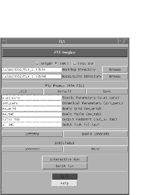
Figure 3: Main FLY TCL window interface to set the fly_fnames file

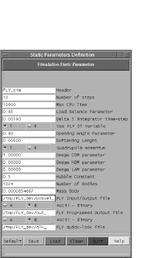
Figure 4: FLY TCL window interface to set the static parameter file

In the main window the user can click on the Generate button and insert data to create the fly_h.F module, the makefiles in the directory src, and the script file that can be submitted to the system queue. The Make button executes the makefile and creates the executable program and the FLY_sort utility.
In the main window it’s also possible to click on the buttons Interactive Run and Batch Run to submit the FLY  execution.

12 FLY tools

FLY  can produce very large output files, whose analysis could be long and cumbersome even on large computing systems. We have then included two utilities which help the user to make some simple analysis using widespread visualization packages, like SuperMongo and IDL. They are contained in the subdirectory tools, and are essentially a C subroutine, slide_3_2d.c, an IDL procedure (slice.pro) and a SuperMongo macro: pl_qlk.
The program slide_3_2d.c is an interactive utility which reads a quick-look input and outputs a file containing densities computed on a grid which is a 2-D projection of a slice of the system along the chosen line-of-sight. The latter is specified as an input parameter. The output is a binary file (slice.d) containing the densities on a grid. For instance, in order to get from a quick-look file qlk_3.0, containing $262144$ positions, a slice along the $y-$direction, on a grid containing $10^{3}$ cells using only particles having $15<y<22.4$ the command would be:

$$\$\,{\rm slices2d-n}\,{\rm qlk\_3.0}\,{\rm-nb}\,262144\,{\rm-nc}\,10\,{\rm-d}\,2\,{\rm-min}\,15$$

$${\rm-max}\,22.4$$

The IDL procedure slice.pro makes isodensity contours of the file slice.d, while the SMongo macro pl_qlk plots the particles on a given slice.
Another tool is the tofly.c routine executing a conversion from big-endian to little-endian and viceversa.

13 Troubleshouting

Using the assistant and the graphical interface, the user sets parameters of the fly_h.F module and uses it to create the FLY  executable. But many other parameters must be adjusted by the user if some errors occur. This section describes the main errors that can occur and the action that must be taken to avoid the error. All the following parameters are included in the fly_h.F module. After any change in the parameter value, FLY  must be re-compiled.

• ch_all error 1: Abort. It is not possible to have the minimum RAM-cache size. Action: there is not enough available memory for this execution. Increase the available memory if it is possible, or decrease the nb_loc (number of local body) or nc_loc (number of local cells) parameter value.

• find_group error 1: overflow. Action: increase the maxilf parameter value, the maximum length of temporary storage to form an Interaction List.

• ilist error 1: overflow. Action: increase the maxnterm parameter value.

• ilist error 2: overflow. Action: increase the maxilf parameter value. If the error will persist, please report the error to the FLY  authors.

• ilist_group error 1: overflow. Action: increase the maxnterm parameter value.

• ilist_group error 3: overflow. Action: increase the maxilf parameter value. If the error will persist, please report the error to the FLY  authors.

• read_params error 1: nbodies greater than nbodsmax. Action: the number value nbodies read from the stat_pars file doesn’t match the nbodsmax parameter. Set nbodsmax equal to nbodies.

• tree_gen error 1: Max level reached: lev greater then nmax_level. Action: The number of levels created to build the tree structure is greater than the maximum allowable levels (equal to lmax). Increase the value of lmax parameter.

• tree_gen error 2: overflow. Action: The number of cells created to build the tree structure, is greater than the maximum allowable internal tree cells (equal to nbodsmax). Increase the value of ncells parameter.

  A complete description of all the errors that can occur is reported in the FLY  User Guide.

14 Conclusion

FLY  is still under development, so many features will be added in the future version. Any question, problem and bug can be reported to the authors sending a detailed e-mail to fly_admin@ct.astro.it, giving a standard test problem, the input parameter files and a description of the system where the bug was found (i.e. operating system, platform, available memory, etc.). An User Guide of FLY  2.1 is available with the FLY  distribution flyug . The FLY  distribution includes a testcase for each supported platform, allowing the user to start a simple demo of a FLY  run. The next public version of FLY  will include the computation of the gravitational potential in an adaptive mesh like Paramesh 1999AAS…195.4203O that will allow the user to interface FLY  outputs with hydrodynamic codes that use adaptive mesh. Moreover a FAQ will be prepared and will be accessible from the FLY  site http://www.ct.astro.it/fly.

References

- [1] U. Becciani and V. Antonuccio Comp. Phys. Com. 136 (2001) 54
- [2] J. Barnes and P. HutNature 324 (1986) 446
- [3] U. Becciani, V. Antonuccio and D. Ferro FLY 2.1 User Guide (2002) http://www.ct.astro.it/fly/,in prepapration
- [4] D.E. Groom The European Physical Journal C15 (2000)
- [5] G. Efstathiou, M. Davis, C.S. Frenk and S.D.M. White ApJS 57 (1985) 241
- [6] S. Carroll astro-ph/0004075 (2000)
- [7] Y. Klypin and H. Holtzmann astro-ph/9712217 (1997)
- [8] E. Bertschinger astro-ph/9506070 (1995)
- [9] L. Hernquist ApJS 64 (1987) 715
- [10] J. E. Barnes and P. Hut ApJS 70 (1989) 389 1989ApJS: Command not found
- [11] K. M. Olson et al. American Astronomical Society Meeting 31 (1999) 1430