Fluctuation Analysis of the Far-Infrared Background -

Information from the Confusion

Yasmin Friedmann^1,2 and Fran${\c{}c}$ois Bouchet³

¹ Racah Institute, The Hebrew University, Jerusalem, 91904, Israel

²Departement de Physique Theorique, University of Geneva

24, quai E. Ansermet, 1211 Geneve 4, Switzerland

³ IAP, 98bis, Bd Arago 75014 Paris, France

We are investigating to what extent one can use a P(D) analysis to extract number counts of unclustered sources from maps of the far infrared background. Currently available such maps, and those expected to emerge in near future are dominated by confusion noise due to poor resolution. We simulate background maps with an underlying two slope model for N(S) and we find that in an experiment of FIRBACK type we can extract the high flux slope with an error of few percent while other parameters are not so well constrained. We find, however, that in a SIRTF type experiment all parameters of this N(S) model can be extracted with errors of only few percent.

1 Introduction

Analysis of spatial fluctuations in the level of background radiation has been used by radio Scheuer (1974); Condon (1974) and x-ray astronomers Barcons & Fabian (1990) to gain information on number count-flux relation below the detection limit.

Recently Lagache et al. (2000), fluctuations in the infrared background were first detected in maps of the FIRBACK survey at wavelength of 170$\mu$m.

Spatial resolution currently available at the far infra-red is of the order of arcminutes. As a result observations at this wavelength are confusion limited. This means that the dominant contribution to noise on sky maps at these wavelengths comes not from detector or photon noise but from the superposition of light originating from galaxies which are too close on the sky to be resolved individually. It has been shown Puget et al. (1999) that the energy coming from resolved sources on the FIRBACK maps comprise only 10$\%$ of the total energy while the rest is due to the unresolved background radiation. This means that other than fluctuation analysis (’P(D) analysis’), not much else can be done to study the N(S) of the unresolved infrared sources at the far infra-red.

This study investigates under which conditions P(D) analysis can usefully constrain galaxy evolution scenarios. Guiderdoni et al. (1998) have introduced a semi-analytical model of galaxy formation and evolution, and within this model suggested several scenarios including different amounts of ultra luminous infrared galaxies. For each of the scenarios they calculated, among other things, faint galaxy counts. They show that at 175 $\mu$m the source counts at fluxes 10-100 mJy are quite sensitive to the details of the galaxy evolution; therefore knowing N(S) to high precision can help choosing between the different scenarios of their galaxy evolution models. Similarly Takeuchi et al. (2001) show that at 175 $\mu$m the number counts at fluxes 10-100 mJy are very dependent on the galaxy evolution models they are suggesting.

When using a simple power law parametrization for the source counts, errors of few percent in the parameters can give an error of  50$\%$ in the number counts at fluxes of few 10s of mJys, i.e. one anticipates that such counts at these flux levels will easily constrain the parameters. Additionally, at least in the above mentioned families of models at this flux range, the N(S) due to the different models differ by an order of magnitude. This justifies attempting to measure the N(S) parameters to high precision down to few 10s mJy. Note that the flux range of few 10s mJy is far below the detection limit of FIRBACK (180 mJy) and therefore, at the moment, can be probed only via P(D) analysis.

Additionnally one would also like to know how much information one can gain about the number counts from specific confusion limited surveys like FIRBACK or SIRTF using a P(D) analysis. This kind of study can be done using a Fisher Matrix Analysis where one calculates the minimal errors of extracted parameters given the experiment and a parameterized theoretical model.

The analysis we make here does not take into account clustering of sources. Some clustering of the far infrared sources is of course expected Knox et al. (2001); Haiman & Knox (2000); Scott & White (1999), but its amplitude is not yet determined at 175 $\mu$m. The small area of the FIRBACK fields might not enable to accurately constrain the source clustering but this situation might change with the SIRTF observations which cover larger areas of the sky Dole et al. (2003). The resolved sources on the FIRBACK maps show a level of clustering consistent with zero. This is probably due to the small number of resolved sources (Guiderdoni and Lagache, private communication). Hence we are assuming, at this stage, that sources are distributed poissonianly on the sky.

We find that we can constrain the slope of the number counts of sources with high fluxes ($\geq~{}20$ mJy) at least as well as has been done by extracting individual strong sources. Other parameters (slope of the number counts at low fluxes, normalization and break flux) are not as well constrained in the FIRBACK type of experiment. However, in an experiment with smaller pixels and more of them (e.g. SIRTF) we can extract all the parameters to within several percent.

We also found some degeneracies between the different parameters and saw that better experiment like SIRTF cannot resolve these degeneracies.

The paper is arranged as follows. We give an explanation of the nature of confusion in sky surveys in section 2. In section 3 we describe how we model the N(S) in order to extract it from the data. In section 4 we outline the method of analyzing sky maps in order to extract the parameters of the model. We describe the implementation of the method and the results of analyzing simulated skies in section 5.

2 Confusion

The spatial fluctuations in the level of background radiation due to spatial distribution of the discrete sources which contribute to the background are called confusion noise. In the far infra-red wavelengths the level of the confusion noise dominates over any photon or instrumental detector noise existing in today’s instruments. Thus while one can reduce the level of instrumental or photon noise by long integration times, the confusion remains a strong characteristic of far-infrared observations.

The full calculation of the probability distribution of the fluctuations (P(D) for short) is classical (see Condon (1974); Barcons & Fabian (1990)) and given in the appendix. Here we only give the final result:

$$P(D)=\int_{-\infty}^{\infty}\Phi(\omega)e^{-2\pi i\omega D}d\omega$$ (1)

where D is the deflection from the mean level of flux and

$$\Phi(\omega)=exp\left[A_{pix}\int_{0}^{\infty}dS\frac{dN}{dS}(S)\sum_{i}\left(e^{2\pi i\omega P_{i}S}-1\right)\right].$$ (2)

The shape of the P(D) depends on several inputs. First is the differential N(S) relation, $\frac{dN}{dS}(S)$. This is the number of sources per steradian with fluxes in [S,S+dS]. It also depends on the shape of the beam, which is described by $P_{i}$. $P_{i}$ is the point spread function of the telescope and $A_{pix}$ is the pixel size.. In general the P(D) will also depend on clustering of the sources if it is strong enough Barcons (1992) but as mensioned before, we are going to deal with a source distribution which is not clustered but Poissonian.

It was shown in Scheuer (1974) that the width of the curve (the 1$\sigma$ of the noise) is of the order of the flux for which there is one source per beam. The very faint sources do not contribute at all to the shape of the curve, but only to the mean level of the flux. This is because there are very many of them within each beam and the change of their number from beam to beam is relatively small and so does not contribute to the fluctuations. The very strong sources contribute only to the tail of the distribution. Typically the flux where there is one source per beam is much lower then the resolution limit.

3 LogN-LogS of infrared sources

Since this work is motivated by the FIRBACK survey we will give in the following a short description of the survey and of the $\frac{dN}{dS}(S)$ found for the resolved sources. These details will guide us when we construct simulations to check our method of deriving $\frac{dN}{dS}(S)$ from the observed P(D).

3.1 The FIRBACK survey

The FIRBACK Puget et al. (1999); Lagache & Dole (2001); Dole et al. (2001) is a deep survey of 4 square degrees of the sky at 170$\mu$m. The 4 degrees were chosen in such a way that the foreground cirrus contamination was as small as possible. Thus one can get information on the extra-galactic radiation Lagache & Puget (2000). In the FIRBACK survey there were 106 sources detected above the sensitivity limit of the experiment at 4$\sigma$, with fluxes between 180 mJy to 2400 mJy. The slope of the LogN-LogS curve was measured by Dole et al. (2001) to be $-3.3\pm 0.6$ between 180 and 500 mJy.

3.2 Modeling Source Counts

In view of the above we will assume a broken power law for the source-count model: the slope at low fluxes has to become shallower than 3.0 or the flux per pixel will diverge. Another motivation for this two slope model is the predictions coming from galaxy evolution models discussed earlier. In all of the predictions the number counts exhibit a relative flattening at low fluxes.

Therefore we write $\frac{dN(S)}{dS}$ as follows:

$$\frac{dN(S)}{dS}=\left\{\begin{array}[]{ll}A_{norm}S^{-\gamma_{1}}&\textrm{for $S\geq S_{break}$}\\ A_{norm}S_{break}^{\gamma_{2}-\gamma_{1}}S^{-\gamma_{2}}&\textrm{for $S_{min}\leq S\leq S_{break}$}\end{array}\right.$$ (3)

The parameters to be determined are the normalization, $A_{norm}$, the flux of the break in the power-law, $S_{break}$, and the two slopes, $\gamma_{1}$ and $\gamma_{2}$. Since $S_{min}$ does not change the shape of the distribution and only affects the mean flux, and since we will be fitting for the shape of the distribution and not for the mean flux, $S_{min}$ becomes irrelevant to the fitting process. It comes into play only in order to fine tune the mean flux to its value from data. In the following we will refer to the four parameters commonly as $\theta$, and the probability distribution of the deflection will be written as P(D;$\theta$).

4 Method of Analysis

4.1 Minimum $\chi^{2}$ Method for Binned Data

Our data set is composed of several thousand measurements of incoming flux received by 46$\times$46 arcsec² pixels which are pointed to different directions in the sky. We will bin the data according to flux. In this way we can compare the experimental distribution of the fluctuations to a calculated P(D;$\theta$).

Binning data may proceed in two ways. One way is such that the bins are equal in length and the number of events vary from bin to bin. Or one may bin the data such that there is the same number of events in each of the bins and the size of the bins changes accordingly. We use the former method but we manually increase the bin size at the two tails of the distribution where there are very few events, so as not to have bins with zero events. We have thus 3 bins where there are around 5 events per bin, out of a total of  60 bins.

A histogram is in fact a multinomial distribution. This is the generalization of the binomial distribution to the case where it is possible to have more then two outcomes for the experiment. In our case the flux received by a pixel pointing in one of the directions in the sky will be one result of the experiment, and the outcome might fall in any one of the bins. Let’s call $r_{1},...r_{n}$ the $n$ possibilities for the outcome of the experiment (in our case $n$ different flux ranges from the minimal to the maximal flux received in the map), and let $p_{i}$ be the probability for a pixel to fall in bin $i$. The sum of all these probabilities is of course 1 since every pixel falls in one of the bins. We assume that the different pixels are independent (we will justify this assumption in section 5.2) . Then, after N experiments of measuring the incoming flux (N pixels in the map), the probability that the fluxes will distribute with $r_{1},...,r_{n}$ pixels falling in the bins will be given by

$$P({r_{i}},N,{p_{i}})=\frac{N!}{r_{1}!r_{2}!...r_{n}!}p_{1}^{r_{1}}p_{2}^{r_{2}}...p_{n}^{r_{n}}$$ (4)

Some important properties of this distribution are that $E(r_{i})$, the expectation value for the bin i, is given by $E(r_{i})=Np_{i}$ and $V(r_{i})$, the variance for bin i is given by $V(r_{i})=Np_{i}(1-p_{i})$. When the number of experiments becomes large the multinomial distribution tends to the multi-normal distribution. In the case when there are many bins and $p_{i}<<1$, the variance tends to be the expectation value. Thus when we bin the fluxes we must take care to have enough bins such that on the one hand $p_{i}<<1$ and on the other, there are enough pixels per bin so that the distribution of the number of pixels per bin will be close to Gaussian. Then the overall likelihood of the data can be written as follows:

$$L(r_{1},....r_{n};\theta)=Ce^{-\frac{1}{2}Q^{2}}$$ (5)

where $Q^{2}$, the quadratic form, is

$$Q^{2}=\sum_{i=1}^{n}\sum_{j=1}^{n}c_{ij}\left(\frac{r_{i}-\mu_{i}}{\sigma_{i}}\right)\left(\frac{r_{j}-\mu_{j}}{\sigma_{j}}\right)$$ (6)

$c_{ij}$ are the elements of the inverse covariance matrix C, given by

$$C=E[(\stackrel{{\scriptstyle\rightarrow}}{{r}}-\stackrel{{\scriptstyle\rightarrow}}{{\mu}})(\stackrel{{\scriptstyle\rightarrow}}{{r}}-\stackrel{{\scriptstyle\rightarrow}}{{\mu}})^{T}]$$ (7)

$r_{i}$ is the number of pixels within flux bin i, $\mu_{i}$ is the expected number of pixels in the bin according to the model, and $\sigma_{i}$ is the square root of the variance, in our case it is $\sqrt{\mu_{i}}$. The correlation $\rho_{i,j}$ between bins i,j is given by

$$\rho_{i,j}=C_{i,j}/\sigma_{i}\sigma_{j}$$ (8)

If we assume that there are no or only negligible correlations between the errors in the bins then the covariance matrix will be almost diagonal. Therefore the quantity we need to minimize becomes

$$Q^{2}=\sum_{i=1}^{N_{bins}}\left(\frac{r_{i}-\mu_{i}}{\sqrt{\mu_{i}}}\right)^{2}$$ (9)

This method is the “minimum chi-square method” applied to histogram fits. When there are many events in each bin then $Q^{2}$ has asymptotically a $\chi^{2}$ distribution with [n-(number of fitted parameters)] degrees of freedom and the method is equivalent to a maximum likelihood estimation method. Therefore from now on we will use the notation $\chi^{2}=Q^{2}$. We are assuming that our way of binning allows $Q^{2}$ to behave close enough to $\chi^{2}$.

4.2 Fisher Matrix Analysis

As described before, we have several thousand measurements of the flux S, and a model for N(S) which leads to a P(D, $\theta$) and we estimate the parameters $\theta$ using maximum likelihood method with the binned data. There is a lower bound to the variance of an estimator, which is related to the Fisher Matrix, $F_{ij}$

$$F_{ij}=E\left[-\frac{\partial logL}{\partial\theta_{i}\partial\theta_{j}}\right]$$ (10)

The Rao-Cramer-Frechet inequality states that for any unbiased estimator, $\Delta\theta_{i}\geq(F^{-1})_{ii}^{1/2}$ where $\Delta\theta_{i}$ is the 1$\sigma$ error of the parameter $\theta_{i}$. This inequality was used by several authors (Jungman et al., 1996; Efstathiou, 1999; Tegmark et al., 1997, e.g.) to assess how well may different parameters be estimated in future experiments.

In our case, where the the likelihood is multinormal, and the errors depend on the parameters, the Fisher matrix becomes Tegmark et al. (1997):

$$F_{ij}=\frac{1}{2}\sum_{k=1}^{N_{bins}}\frac{\partial\mu_{k}}{\partial\theta_{i}}\frac{\partial\mu_{k}}{\partial\theta_{j}}\frac{1}{\mu_{k}}\left[2+\frac{1}{\mu_{k}}\right]\bigg{|}_{\theta_{ML}}$$ (11)

As we can see, the Fisher matrix depends solely on the model and on the estimated parameters, $\{\theta_{ML}\}$. We can now calculate the minimal variance for different experimental setups, namely as a function of the number of pixels in the maps, or as a function of the size of the pixel. In this way we can foresee how well we could extract the 4 parameters from future experiments.

The inverse of the Fisher matrix is an estimate of the covariance matrix, so by investigating F^-1 one can locate degeneracies between parameters and see if they might be resolved in different experimental setups.

5 Results

In this section we describe the analysis of simulated skies that we have made in order to check theoretically the limits of our method using the fisher matrix analysis.

5.1 Simulations

We use mock images to check our algorithm. These images are built in two steps. First we build a mock sky. This is a high resolution projected image of a given spatial distribution of sources. It is constructed by distributing point sources randomly on a $1.25\times 1.25$ square degree field. Each source is assigned a flux such that the overall number counts are consistent with our predetermined two-slope N(S). We chose to model N(S) such that the main traits of the FIRBACK maps are realized, such as the number of sources above 180mJy and the mean level of the background. Then we convolve it with the instrumental effects in order to produce an image as close as possible to real data. Finally we extract only the central 1 square degree as our map. A map produced this way is presented in figure 1 (a), and its histogram is shown in 1(b). The map includes some $2*10^{8}$ sources with fluxes ranging from 0.01 to 2000 mJy, and the parameters chosen were $\gamma_{1}=3.3$, $\gamma_{2}=1.8$ and $S_{break}=14$mJy and the normalization was 0.18*$10^{11}$.

$\begin{array}[]{cc}\lx@intercol\hfil\lx@intercol&\lx@intercol\hfil\lx@intercol\\ \includegraphics[width=199.16928pt]{marveloustest.ps}&\includegraphics[width=199.16928pt]{histo9_4.ps}\\ \end{array}$

Figure 1: Left: 1 square degree of simulated sky, with pixels of 46² arcsec². The sky contains some $2*10^{8}$ sources, described by a model N(S) given in equation 3, with parameters as follows: $\gamma_{1}=3.3$, $\gamma_{2}=1.8$, $S_{break}=14$mJy and $A_{norm}=0.18*10^{11}$. Right: The histogram of the simulated map showing the fluctuations in the intensity. Note the skewed shape, with the tail due to the strong sources.

5.2 Effect of Different PSFs on Correlation Between Flux Bins

The total extent of the PSF of the FIRBACK instrument and of the upcoming SIRTF is bigger then the size of a pixel in these experiments. In FIRBACK the Full Width at Half Maximum of the PSF is equal to the pixel size. For SIRTF it is twice as wide Dole et al. (2003). In such cases we expect there to be some correlation between adjacent pixels on the map. Given this, we want to quantify to what extent these correlations may be manifested as correlations between the different bins in the histogram.

To this end we should measure the correlation coefficients of the histogram given different sized PSFs. The different PSFs we used were constructed from the original one by rebinning again and again. We quantify their extent with respect to the pixel size by defining variable x which is the ratio of the FWHM to the pixel size. The x we used are 2.7, 1.1, 0.5, 0.3 and 0.1. Following this we produced hundreds of sky maps based on the same underlying N(S) relation. We convolved each with a FSF, produced a histogram, and measured the sample correlation matrix. The process was repeated for the different PSFs, and was done once without convolving with any PSF but instead we rebinned the sky to the size of the pixel, 46”$\times$ 46”.

If bins were not correlated at all, the correlation matrix would have been the identity matrix. We found that there is a negligible level of correlations with any of the PSFs, mostly less than 10$\%$. The largest correlation seen was between few neighboring bins for the largest PSF, near the center of the histogram, at a level of  20$\%$. There is also no clear behavior of $\rho_{ij}$ as a function of the total coverage area of the PSF. This can be seen in figure 2, where 3 randomly selected elements of the correlation matrix are plotted as a function of the total coverage area of the PSF.

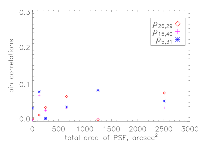
Figure 2: Three randomly chosen elements of the correlation matrix, plotted as a function of the total coverage area of the PSF. All correlations are less then 10$\%$, and there is no clear trend of behavior as a function of the coverage.

In light of this we will neglect the correlations between the bins and estimate the parameters as described in the next section.

5.3 Estimating Parameters

In order to find estimates for the 4 parameters $A_{norm},S_{break},\gamma_{1},\gamma_{2}$, we first choose a small enough value for $S_{min}$. On the one hand it should be smaller then reasonable values of $S_{break}$, and on the other hand it should be big enough to avoid numerical problems of integration. We then grid a large enough part of parameter space around a reasonable point found by trial and error. Each of these grid points will serve as a starting point for the minimization procedure. This way we have more chance of catching the lowest minimum. The minimization procedure calculates the $\chi^{2}$ and uses the derivatives of the model to go downhill in parameter space until a lowest local $\chi^{2}$ is found. We looked at the estimated parameters and their errors to see whether they are all situated in the same part of the parameter space. We repeated the procedure with several different binning to make sure that the results are not dependent on the binning. The best fit is shown in figure 3. The reduced $\chi^{2}$ for this model is 0.96. The errors of the estimated parameters will be discussed below.

Once we have a best fit set of parameters, we assume that it is a good enough approximation of the real parameters. Then we can continue to calculate the fisher matrix elements for different experimental parameters. We will calculate the minimal errors of the different parameters as a function of pixel size and as a function of the number of pixels in the map.

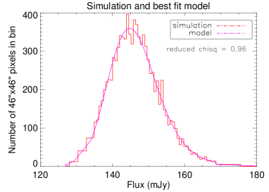
Figure 3: Here we see again the histogram of the simulated map with the best fit model

In fig. 4a one sees how the errors reduce when we add more pixels to the map. In fact they reduce as (number of pixels)^-1 - and this behavior is what we expect from the definition of the fisher matrix, equation 11.

$\begin{array}[]{c@{\hspace{0.1in}}c}\lx@intercol\hfil\lx@intercol&\lx@intercol\hfil\lx@intercol\\ \includegraphics[width=199.16928pt]{all_errors_vs_map_size_17_9.ps}\hfil\hskip 7.22743pt&\includegraphics[width=199.16928pt]{all_errors_vs_pix_size_17_9.ps}\\ \mbox{(a)}\hfil\hskip 7.22743pt&\mbox{(b)}\end{array}$

Figure 4: Shown are the errors on the estimated parameters (in percent) as a function of the number of pixels in the map (a) and as a function of the pixel size (b). The vertical line shows where the FIRBACK experiment is on these grafs.

In fig. 4b one sees that the errors greatly reduce once we use smaller pixel sizes in the experiment, with all errors at the level of only few percent once we reach pixel size of 15 arcsec². This is very encouraging because in the upcoming SIRTF experiment the pixels will be of size $16\times 16$ arcsec².

Another point to look at is the comparison between the errors on the estimated parameters in our algorithm, and the minimal errors given from the Fisher Matrix analysis. To this end we plotted, on both 4a and 4b a vertical line indicating the properties of the FIRBACK and our simulations. On top of this line we put the parameter errors we got from the minimization procedure. It is encouraging to see that these errors are only very slightly larger than the minimal errors possible according to the Cramer-Rao-Frechet lower bound.

Another way to see the great improvement in the precision of the estimation is when one looks at the 1$\sigma$ contours which enclose 68$\%$ of the joint distribution of several pairs of estimators while we marginalize over the other two parameters, as in fig. 5. The contours, independent of which plane we look at, encompass a shrinking patch of the parameter space as we add pixels to the map or use smaller pixels. We have plotted the original parameters as filled hexagons on top of the ellioses. It is important to note, also, that except for the normalization, the true parameters of the simulation are enclosed within the 1$\sigma$ contours of the original experiment.

5.4 Parameter Degeneracies

Figure 5 also shows us that there are degeneracies between the different parameters. These degeneracies are not broken when we use a more accurate experiment, they are “built in” through the definition of the model N(S). For example, as the model is defined, the normalization is the number of sources with fluxes greater than 1mJy. Naturally, if we increase $\gamma_{1}$ we should increase the normalization in order to remain within the error bars for N(S).

$\begin{array}[]{c@{\hspace{0.1in}}cc}\lx@intercol\hfil\lx@intercol&\lx@intercol\hfil\lx@intercol&\lx@intercol\hfil\lx@intercol\\ \includegraphics[width=142.26378pt]{ellipse_norm_g1_18_9.ps}\hfil\hskip 7.22743pt&\includegraphics[width=142.26378pt]{ellipse_sb_g2_18_9.ps}&\includegraphics[width=142.26378pt]{ellipse_sb_g1_18_9.ps}\\ \mbox{(a)}\hfil\hskip 7.22743pt&\mbox{(b)}&\mbox{(c)}\end{array}$

Figure 5: Here we present the 1$\sigma$ contours in the two dimensional plane of 3 different pairs of parameters, while marginalizing over the rest. These contours are calculated according to F^-1. The filled hexagons give the original parameters of the simulation on these planes.

In the following we will look further into the degeneracies by looking at the derivatives of the model with respect to the parameters we are interested in Tegmark et al. (1997). The reason for this can be seen if we look again at the expression for the elements of the Fisher Matrix (eq.11): they have the structure of a dot product between vectors $\frac{\partial\mu_{k}}{\partial\theta_{i}}$ and $\frac{\partial\mu_{k}}{\partial\theta_{j}}$ . If one of these vectors is a linear combination of another, the Fisher matrix elements will be singular, and the errors of the estimated parameters will be infinite. If the vectors are completely orthogonal then F and F^-1 will be diagonal and thus there will be no correlation between different parameters and their errors. Usually there will be some level of correlation which will be manifested by a somewhat similar shape between the functional shape of the different derivatives. By looking at the functional shape of the derivatives one may recognize such degeneracies. The way to avoid any degeneracies between parameters will be to diagonalize the Fisher Matrix, thus changing the parameters into new ones which are linear combinations of the originals. These parameters, however, are not always physical, and thus do not have much meaning unless they are very similar to the old ones, with not much ‘contamination’ from other parameters.

It is worthwhile to check whether under improved experimental conditions these degeneracies, if they exist, are removed or not. In fig 6 we plot the derivatives with respect to the usual 4 parameters and the derivatives with respect to the new, “diagonalised” parameters (called principal components - PC1-4). On the left panel we have the case for a pixel of 20*20 arcsec², and on the right, 46*46 arcsec². Again we can see that the degeneracies are not removed by improving the experiment. Only diagonalizing the fisher matrix allows us to remove them.

$\begin{array}[]{c@{\hspace{0.1in}}c}\includegraphics[width=199.16928pt]{N_ders_20_together.ps}\hfil\hskip 7.22743pt&\includegraphics[width=199.16928pt]{N_ders_46_together.ps}\\ \includegraphics[width=199.16928pt]{N_PC_ders_20.ps}\hfil\hskip 7.22743pt&\includegraphics[width=199.16928pt]{N_PC_ders_46.ps}\\ \mbox{(a)}\hfil\hskip 7.22743pt&\mbox{(b)}\end{array}$

Figure 6: The top figures show the derivatives of the model with respect to the 4 parameters at 2 pixel sizes - 46²” and 20²”. the bottom show the derivatives of the model with respect to the principal components. It is possible to see how the degeneracies disappear.

We also add a table which specifies how the new parameters are built from the old ones. In the first row we have the 4 parameters and in the first column we have the 4 principal components. In each of the 4 rows we have the coefficients of the linear combination. The strongest coefficients are marked in bold.

$$\bordermatrix{&K&\gamma_{1}&\gamma_{2}&S_{break}\cr PC1&0.32&{\bf 0.91}&0.24&-0.03\cr PC2&{\bf 0.94}&-0.34&0.03&-0.004\cr PC3&-0.11&-0.21&{\bf 0.96}&-0.09\cr PC4&0.0015&0.002&0.098&{\bf 0.995}}$$

PC1 has the highest weight from $\gamma_{1}$ with some contribution from $K$ and $\gamma_{2}$. PC2 has the highest contribution from $K$ and some contribution from $\gamma_{1}$. PC3 is mostly $\gamma_{2}$ and some $\gamma_{1}$, and PC4 is almost exclusively $S_{break}$. The degeneracies are to be expected since as mentioned before, P(D) analysis cannot give information at fluxes much below the one source per beam flux level. In our simulation this level is of the order of 7mJy and therefore it is reasonable that for example $\gamma_{2}$, which is the slope of the counts below a few mJy is degenerate with the other parameters.

6 Discussion

In this work we have explored the extent to which one can use a P(D) analysis to gather information from far infra red sky maps. These maps are characterized by a very high level of confusion noise which arises due to the relatively poor resolution power available at these wavelengths.

We created a simulated map of the sky with an underlying modeled N(S). The model consisted of a two slope model with a high flux slope greater than 3 and a shallower low-flux slope. It was chosen this way following the finding of a steep slope of the number counts of resolved objects in the FIRBACK maps and in agreement with predictions of galaxy evolution models. The parameters of the model are the two slopes, the break flux (where the slope changes) and the normalization.

We then created the histogram of the simulated map and used it to find the best fit parameters of the N(S) model and their errors. After finding the best fitted parameters, we used the Fisher matrix analysis to calculate the minimal errors possible of these parameters in experiments with different pixel sizes and in experiments with different total number of pixels, including those of the FIRBACK.

We found that our algorithm gives fitted parameters with almost the minimal errors possible theoretically. The underlying parameters of the simulated map were within 1$\sigma$ of the best fitted ones (except for the normalization). This means that the tool we have constructed in order to find number counts is quite reliable.

The Fisher Matrix analysis shows that in an experiment with pixel size of the order  10 arcsec we will be able to find all parameters with errors of only about a few percent. The situation of the FIRBACK experiment is quite different: it is only the high flux slope which can be found with a small error bar of $\approx$4$\%$. This is somewhat better than what was found by individual source extraction from the maps (error of $\approx$20$\%$).

The advantage of the P(D) analysis that it is sensitive down to the flux for which there is one source per beam - in the FIRBACK case this is around few mJy, much below the detection limit which is 180mJy. Also, the extraction of even the high flux slope is straightforward and does not warrant an a-priory extraction of sources or other manipulation of the maps.

In order to be able to extract the other parameters of the number counts, we will have to wait for the SIRTF experiment. In that experiment, the pixel size is 16”*16” and the number of different points measured on the sky is up an order of magnitude larger then for FIRBACK. In this case the precision of estimation is enhanced due to both factors: smaller pixels and more of them.

Appendix A Probability Distribution of Background Fluctuations

The shape of the curve describing the probability that a pixel will accumulate a certain level of flux depends on a few factors. These are the point spread function of the telescope, the pixel size and shape, and the source number counts N(S).

We are assuming some properties for the sources which make up the background: that the sources are point-like, they are not clustered, and once a source is “found” its flux is a random variable distributed according to the number-count-flux relation, $N(S)$.

The integrated flux seen by a pixel pointing in direction n will be:

$$S_{pix}({\mbox{\bf n}})=\int d\Omega_{{\mbox{\bf n'}}}G({\mbox{\bf n}}-{\mbox{\bf n'}})S({\mbox{\bf n}}^{\prime})$$ (12)

$d\Omega_{{\mbox{\bf n}}}$ is the solid angle in direction n. G$({\mbox{\bf n}}-{\mbox{\bf n'}})$ is the beam profile - it is the convolution of the point spread function of the imaging instrument and the pixel profile. $S({\mbox{\bf n}})$ is the flux per unit solid angle coming from direction n. Now we can calculate the probability density of $S_{pix}$ (the probability that a certain pixel will receive flux $S_{pix}$). In order to do that one first calculates the characteristic function of $S_{pix}$ which is given by

$$\Phi(\omega)=<e^{2\pi i\omega S_{pix}}>$$ (13)

Then the probability distribution for $S_{pix}$ will simply be the Fourier transform of $\Phi$.

Say there are K sources. Then the total flux received by a pixel should be written as the following discrete sum:

$$S_{pix}(\mbox{\boldmath$n$})=\sum_{i=1}^{k}S_{i}G(\mbox{\boldmath$n$}-\mbox{\boldmath$n_{i}$})$$ (14)

The probability of finding K sources in the sky, with fluxes $S_{1},...S_{k}$ and in directions ${\bf n_{1}}$,…${\bf n_{k}}$, is

$$F^{(k)}(\mbox{\boldmath$n_{1}$},S_{1}...\mbox{\boldmath$n_{k}$},S_{k})=\frac{(4\pi\mu)^{k}}{k!}e^{-4\pi\mu}(4\pi)^{-k}\prod_{i=1}^{k}f(S_{i})$$ (15)

$\mu$ is the mean number of sources per unit solid angle, and $f(S)$ is the probability that a source has a flux in the range $[S,S+dS]$. This is a product of the Poissonian probability to find K sources while the mean number of sources is expected to be $\mu$ and the probability to find a source with flux $S_{i}$ given the model N(S), all this per steradian (hence the term $(4\pi)^{-K}$. The normalization condition is that the sum of the probabilities to find any number of sources in any direction is one:

$$\sum_{k=0}^{\infty}\int d\Omega_{n_{k}}\int_{0}^{\infty}dS_{1}...\int d\Omega_{\mbox{\boldmath$n_{k}$}}\int_{0}^{\infty}dS_{k}F^{(k)}(\mbox{\boldmath$n_{1}$},S_{1};...\mbox{\boldmath$n_{k}$},S_{k})=1$$ (16)

Using the normalization condition and the form of $S_{pix}$ we may now calculate the characteristic function, which becomes:

$$\Phi(\omega)=exp\left[A_{pix}\int_{0}^{\infty}dS\frac{dN}{dS}(S)\sum_{i}\left(e^{2\pi i\omega P_{i}S}-1\right)\right]$$ (17)

$P_{i}$ is the pixelized PSF and $A_{pix}$ is the area of the pixel in steradians. The integration over the angles is separate from that over flux and gives $A_{pix}$. This is justified in our case because although the PSF is quite extended, outside of the pixel it has very small values. So now we may write the expression for the P($S_{pix}$), as the Fourier transform of the characteristic function:

$$P(S_{pix})=\int_{-\infty}^{\infty}\Phi(\omega)e^{-2\pi i\omega S_{pix}}\omega$$ (18)

The above expression gives the probability that a pixel will receive an amount of flux equal to $S_{pix}$. We will be working with a slightly different expression - the probability to get a certain flux above or below the mean flux on the map, $D$, defined as $S_{pix}=D+<S_{pix}>$

$$P(D)=\int_{-\infty}^{\infty}\Phi(\omega)e^{-2\pi i\omega D}\omega$$ (19)

Once we have P(D) we may integrate between the bins and multiply by the total number of pixels in the map to get the expected number of pixels falling within each bin.

References

- Barcons (1992) Barcons, X. (1992). Confusion noise and source clustering. ApJ, 396, 460–468.
- Barcons & Fabian (1990) Barcons, X. & Fabian, A. C. (1990). A fluctuation analysis of the X-ray background in the Einstein Observatory IPC . MNRAS, 243, 366–371.
- Condon (1974) Condon, J. J. (1974). Confusion and Flux-Density Error Distributions. ApJ, 188, 279–286.
- Dole et al. (2001) Dole, H., Gispert, R., Lagache, G., Puget, J.-L., Bouchet, F. R., Cesarsky, C., Ciliegi, P., Clements, D. L., Dennefeld, M., Désert, F.-X., Elbaz, D., Franceschini, A., Guiderdoni, B., Harwit, M., Lemke, D., Moorwood, A. F. M., Oliver, S., Reach, W. T., Rowan-Robinson, M., & Stickel, M. (2001). FIRBACK: III. Catalog, source counts, and cosmological implications of the 170 mu m ISO. A&A, 372, 364–376.
- Dole et al. (2003) Dole, H., Lagache, G., & Puget, J.-L. (2003). Predictions for Cosmological Infrared Surveys from Space with the Multiband Imaging Photometer for SIRTF. ApJ, 585, 617–629.
- Efstathiou (1999) Efstathiou, G. (1999). Constraining the equation of state of the Universe from distant Type Ia supernovae and cosmic microwave background anisotropies. MNRAS, 310, 842–850.
- Guiderdoni et al. (1998) Guiderdoni, B., Hivon, E., Bouchet, F. R., & Maffei, B. (1998). Semi-analytic modelling of galaxy evolution in the IR/submm range. MNRAS, 295, 877–898.
- Haiman & Knox (2000) Haiman, Z. & Knox, L. (2000). Correlations in the Far-Infrared Background. ApJ, 530, 124–132.
- Jungman et al. (1996) Jungman, G., Kamionkowski, M., Kosowsky, A., & Spergel, D. N. (1996). Weighing the universe with the cosmic microwave background. Physical Review Letters, 76, 1007–1010.
- Knox et al. (2001) Knox, L., Cooray, A., Eisenstein, D., & Haiman, Z. (2001). Probing Early Structure Formation with Far-Infrared Background Correlations. ApJ, 550, 7–20.
- Lagache & Dole (2001) Lagache, G. & Dole, H. (2001). FIRBACK. II. Data reduction and calibration of the 170 m ISO deep cosmological survey. A&A, 372, 702–709.
- Lagache & Puget (2000) Lagache, G. & Puget, J. L. (2000). Detection of the extra-Galactic background fluctuations at 170 mu m. A&A, 355, 17–22.
- Lagache et al. (2000) Lagache, G., Puget, J., Abergel, A., Desert, F., Dole, H., Bouchet, F. R., Boulanger, F., Ciliegi, P., Clements, D. L., Cesarsky, C., Elbaz, D., Franceschini, A., Gispert, R., Guiderdoni, B., Haffner, L. M., Harwit, M., Laureijs, R., Lemke, D., Moorwood, A. F. M., Oliver, S., Reach, W. T., Reynolds, R. J., Rowan-Robinson, M., Stickel, M., & Tufte, S. L. (2000). The Extragalactic Background and Its Fluctuations in the Far-Infrared Wavelengths. In ISO Survey of a Dusty Universe, Proceedings of a Ringberg Workshop Held at Ringberg Castle, Tegernsee, Germany, 8-12 November 1999, Edited by D. Lemke, M. Stickel, and K. Wilke, Lecture Notes in Physics, vol. 548, p.81, pages 81–+.
- Puget et al. (1999) Puget, J. L., Lagache, G., Clements, D. L., Reach, W. T., Aussel, H., Bouchet, F. R., Cesarsky, C., Désert, F. X., Dole, H., Elbaz, D., Franceschini, A., Guiderdoni, B., & Moorwood, A. F. M. (1999). FIRBACK. I. A deep survey at 175 microns with ISO, preliminary results. A&A, 345, 29–35.
- Scheuer (1974) Scheuer, P. A. G. (1974). Fluctuations in the X-ray background. MNRAS, 166, 329–338.
- Scott & White (1999) Scott, D. & White, M. (1999). Implications of SCUBA observations for the Planck Surveyor. A&A, 346, 1–6.
- Takeuchi et al. (2001) Takeuchi, T. T., Ishii, T. T., Hirashita, H., Yoshikawa, K., Matsuhara, H., Kawara, K., & Okuda, H. (2001). Exploring Galaxy Evolution from Infrared Number Counts and Cosmic Infrared Background. PASJ, 53, 37–52.
- Tegmark et al. (1997) Tegmark, M., Taylor, A. N., & Heavens, A. F. (1997). Karhunen-Loeve Eigenvalue Problems in Cosmology: How Should We Tackle Large Data Sets? ApJ, 480, 22–+.