Morphology of Mock SDSS Catalogues

Abstract

We measure the geometry, topology and morphology of the superclusters in mock SDSS catalogues prepared and reported by Cole et al.(1998). The mock catalogues refer to $\tau$CDM and $\Lambda$CDM flat cosmological models and are populated by galaxies so that these act as biased tracers of mass, conforming with the observed two-point correlation function measured using APM catalogue on scales between 1 to 10 h^-1Mpc. We compute the Minkowski Functionals (hereafter, MFs) for the cosmic density fields using SURFGEN (Sheth et al.2003) and use the available 10 realizations of $\tau$CDM to study the effect of cosmic variance in estimation of MFs and Shapefinders; the statistics derived from MFs, and used to study the sizes and shapes of the superclusters. The MFs and Shapefinders are found to be extremely well constrained statistics, useful in assessing the effect of higher order correlation functions on the clustering of galaxy-distribution. We show that though all the mock catalogues of galaxies have the same two-point correlation function and similar clustering amplitude, the global MFs due to $\tau$CDM show systematically lower amplitude compared to those due to $\Lambda$CDM, an indirect, but detectable effect due to nonzero, higher order correlation functions. This enables us to successfully distinguish the two models of structure formation.

We further measure the characteristic thickness (T), breadth (B) and length (L) of the superclusters using the available 10 realizations of $\tau$CDM. While T$\leq$B and T, B$\in$[1,17] h^-1Mpc, we find the top 10 superclusters to be as long as 90 h^-1Mpc, with the longest superclusters identified at percolation to be rare objects with their length as large as 150 h^-1Mpc. The dominant morphology of the large superclusters is found to be filamentary. The thickness, breadth and planarity of the superclusters follow well-defined distributions which are different for the two models. Thus, these are found to be sensitive to the cosmological parameter-set and are noted to be candidate statistics which can compare the rival models of structure formation. Further, the longest structures of $\tau$CDM are found to be significantly longer than those in $\Lambda$CDM. Finally, mass and volume-weighted dimensionless Shapefinders – Planarity and Filamentarity – are found to be well-constrained statistics useful to discriminate the two models. We note some interesting effects of bias and stress the importance of incorporating realistic treatment of bias in preparing and analysing the mock catalogues.

1 Introduction

The present era marks a remarkable milestone in the history of Cosmology due to an alround increase in the extragalactic database by several orders of magnitude over last few years. These data have improved both in quantity and in quality, due to which theoretical models of the Universe are directly confronted with the observations, either to be validated or to get more refined. The primordial density fluctuations as revealed imprinted on the otherwise smooth and isotropic microwave background radiation (MBR) have been measured with unprecedented accuracy and resolution by WMAP (Bennett et al., 2003), thus enabling us to obtain the most reliable estimates of the cosmological parameters and confirming that the geometry of the Universe is indeed flat. An independent constraint from the study of extragalactic distances using type-Ia supernovae seems to indicate that we live in a low matter-density, cosmological constant dominated Universe, with $\Omega_{\Lambda}\approx$0.7. A variety of observations like, the power spectrum study of the MBR, the clustering properties of the galaxy-distribution and the rotational velocity measurements in normal-size galaxies as well as in the clusters of galaxies (Kneib et al., 2003), all seem to indicate that most of the remaining fraction of the matter-density is in the form of dark matter which is nonrelativistic, i.e., cold in nature. Thus, the cosmological constant dominated, Cold Dark Matter model ($\Lambda$CDM) seems to be the best fitting cosmological model of the Universe that we inhabit. However, several anamolies have surfaced which cannot be easily reconciled with the hypothesis of cold dark matter. For example, an order-of-magnitude lower than predicted number density of dwarf or low surface brightness galaxies observed in the local Universe, the mismatch between the predicted and the observed density profiles of these galaxies, the lack of sufficient substructure in normal size galaxies, going against the standard hierarchical model of structure formation, etc. are not readily explained within the standard CDM paradigm and secondary physical processes are sought to explain many of these anomalies. Hence, the issues related to structure formation and background cosmology are likely to have a vigorous interplay with the physics of galaxy formation, a process which may lead to deeper insights into our ideas about the cosmological model(s) of the Universe. It suffices, hence, to devise algorithms and statistics which enable us to compare our theoretical predictions with a variety of observations of the Universe.

The developments on studying the microwave background radiation are further complemented by properties of the large scale structure revealed by increasingly deep and voluminous redshift surveys. Indeed, redshift surveys continue to occupy a central place in our efforts to understand the Universe for, as opposed to CMBR which gives us a view of the early Universe, these provide us with a view of the matter-distribution in our immediate extragalactic neighbourhood. In addition to revealing the large-scale distribution of galaxies, a redshift survey provides us with a statistically fair sample to estimate many properties associated with various galaxy-populations, e.g., the luminosity function (Blanton et. al., 2003; Norberg et al., 2002a), the clustering of galaxies of various “types” (Norberg et al., 2002b), the mass-to-light (M/L) ratio in galaxies of different morphological or spectral types (for example, Brainerd & Specian 2003), etc. Further, with the help of efficient algorithms, it is possible to identify groups and clusters of galaxies and assess the role which their environments play in the evolution of their constituent galaxies . Such findings provide crucial feedback to our efforts in understanding the physics of galaxy formation. For a detailed review highlighting potential applications and importance of redshift surveys in the study of the Universe, see a recent review-article by Lahav & Suto (2003).

Whereas the paradigm of structure formation due to gravitational instability has been explored to a great extent, both analytically and using N-body simulations, these studies have mainly focussed on the dynamics of the dark matter. However, we now have richer quality and quantity of data with which to confront our theoretical models. For example, the 2 degree field galaxy redshift survey (2dFGRS) containing about 250 000 galaxies and covering about 1500 square degree of the sky is complete (Colless et al.2003), while the Sloan Digital Sky Survey (SDSS) team has recently made its first data release (FDR) reporting the redshifts of about 180 000 galaxies (Abazajian et al., 2003). When complete, the SDSS will cover about a quarter of the full sky and reveal the distribution of a million galaxies upto 600 h^-1 Mpc, a depth comparable to that attained by 2dFGRS.

In light of the above developments, the attention of the cosmology community has steadily shifted to simulating the formation of galaxies in dynamically evolving dark matter background. In this context, it is worth mentioning two widely adopted approaches – the semi-analytic galaxy formation methods (Cole et al., 2000; Benson et al., 2002) and SPH methods (Weinberg, Hernquist & Katz, 2002). However, these two approaches do have their own limitations (Berlind et al.2003), and important insights have been obtained by a complementary approach based on the Conditional Luminosity Function (see Yang, Mo, van den Bosch & Jing 2003 and a series of earlier papers by this group).

The catalogues of “galaxies” prepared using the methods advocated by these teams are to be tested against the large body of observations due to deep, upcoming redshift surveys. Such a comparison should have two main aims:

1. To employ various population statistics which reflect the structural properties of the ensemble of galaxies. These are mainly the kinematic measures defined for a given sample of a large number of galaxies. The luminosity function, the mass-to-light ratios of galaxies of various morphological or spectral types, mass-to-light ratios of groups/clusters, the morphology-density relation etc. form this class of measures and are chiefly used to validate/invalidate a mock catalogue.

2. To assess the large-scale distribution of galaxies and to quantify the clustering of the ensemble of galaxies. The two-point correlation function, the three-point correlation function, the pair-wise velocity dispersion, etc. are the most widely used statistics belonging to this category. These statistics reflect the dynamical history and clustering properties of the matter-distribution.

The list of statistics which fall in the latter category is, however, not complete. The statistical properties of the primordial gaussian random phase density field are fully quantified in terms of its power spectrum, or its Fourier counterpart, the two-point correlation function. However, a subsequent gravitational dynamics introduces phase correlations among the neighbouring density modes of this density field (Sahni & Coles, 1995). This is accompanied by a transfer of power from larger scales to smaller scales (Hamilton et al., 1991) as a result of which the entire hierarchy of correlation functions becomes nonzero. Hence, a full quantification of the large scale cosmic density field at today’s epoch would ideally require us to have knowledge of all the higher order correlation functions. Under appropriate assumptions, analytic treatment goes as far as predicting the effect of gravitational dynamics on the 3-point correlation function, or at best the 4-point correlation function, but not beyond. It is to be noted that even this treatment is within the perturbative regime and breaks down when the density contrast exceeds unity. However, we note that a mock catalogue could not be satisfactorily compared with the real cosmic density field merely by a subset of correlation functions for which analytic predictions are available. In fact, most of the N-body simulations are structure-normalised so as to reproduce the current rich cluster abundance observed in our neighbourhood. In addition, mock catalogues constructed from N$-$body simulations are usually required to reproduce the observed two-point galaxy-galaxy correlation function (Cole, Hatton, Weinberg, & Frenk, 1998; Yang, Mo, van den Bosch & Jing, 2003). Thus, the mock catalogues of various cosmological model(s) agree with the large scale structure (hereafter, LSS) of the Universe by construction, and cannot be discriminated from one another or from the observed LSS of the Universe on the sole basis of the 2-point correlation function. We might add that higher order correlation functions (beyond, say, the three-point correlation function) are cumbersome to estimate for a system comprising of large number of particles. Furthermore, the correlation functions offer us little intuitive insight to guide us in interpreting the results. Thus, distinctly different statistics are needed to give us an handle on the effect of higher order correlation functions. It is desirable that these statistics simultaneously offer us an intuitively clear interpretation as well as allow us for their numerically robust estimation.

In this paper, we propose to use one such class of measures – the Minkowski Functionals (hereafter, MFs) (Mecke, Buchert & Wagner, 1994; Sheth et al., 2003) and related morphological statistics, the Shapefinders (Sahni, Sathyaprakash & Shandarin, 1998) – to quantify and characterise the large scale distribution of galaxies. Our main motivation in using the MFs for this purpose is that (1) MFs have been shown to be dependent on the entire hierarchy of correlation functions (Mecke, Buchert & Wagner, 1994; Schmalzing, 1999), and (2) the MFs in both 2$-$D and in 3$-$D have physically important interpretation, namely that out of ($n+$1) MFs available in $n-$D, the first $n$ of them characterise the geometry of the excursion set under question (these could be superclusters or voids of the cosmic web, for example) and the remaining MF is sensitive to the topology or the connectedness of the associated hypersurface. In recent times, there is even more motivation for employing MFs for the quantification of LSS after Matsubara (2003) derived the MFs for cosmic density fields in the weakly nonlinear regime using 2^nd order Euler perturbative expansion. With the availability of large datasets like 2dFGRS and SDSS, it should be possible to test these predictions by working with the cosmic density fields smoothed at sufficiently large length-scales .

Various attempts have been made to quantify the cosmic web using MFs (Bharadwaj, et. al., 2000; Sheth et al., 2003; schmlzpap99). The efficacy of MFs in quantifying cosmic density fields as well as in making a morphological survey of the structural elements of the cosmic web – superclusters – has thereby been abundantly demonstrated. Recently, Hikage et al. (2003) provided Minkowski Functionals for SDSS (EDR). Further, Basilakos (2003) used Shapefinders to study the morphology of the superclusters in SDSS(EDR) and found the dominant morphology of the superclusters to be filamentary. In the mean time, important advances have been made concerning techniques to calculate the MFs. The grid-based techniques based on the Crofton’s formulae or the Koenderink invariants (Schmalzing & Buchert, 1997) have been recently complemented by a powerful, triangulation based surface-generating method which self-consistently generates isodensity contours for a density field defined on a grid. This method also makes possible an online computation of the MFs. The method, the associated software SURFGEN, its accuracy and application to a class of N$-$body simulations were reported in a recent paper by Sheth et al. (2003).

In this paper, we analyse the LSS in the SDSS mock catalogues corresponding to two models of structure formation – $\Lambda$CDM and $\tau$CDM. These mock catalogues were prepared by Cole et al.(1998) (hereafter, CHWF) based on various physically motivated biasing schemes represented in terms of analytic functions. The biasing schemes were used to prescribe the “formation-sites” of the galaxies for a given cosmological density field. Despite being superseded by semi-analytic and Conditional Luminosity Function based techniques to develop more realistic mock catalogues, till date these catalogues have several advantages to their credit. This is because, these catalogues fulfill several kinematic as well as dynamical constraints. For example, the survey geometry and the b_J band luminosity functions for both 2dFGRS and SDSS have been incorporated, ensuring an accurate reproduction of the expected radial selection function in both the cases . In addition, these catalogues mimic the survey geometry of both 2dFGRS and SDSS, thus pausing the associated challenges in the subsequent analysis of the LSS, and preparing one for the analysis of the actual survey data. Further, the mock catalogues due to all the models and due to all the various biasing schemes were constrained to reproduce the two-point correlation function (Baugh, 1996) and the power spectrum (Baugh & Efstathiou, 1993) derived from the APM catalogue. The library of catalogues is impressive, both due to a wide coverage of the cosmological models which it offers, as well as in providing data due to a variety of biasing schemes, all consistent with the actual LSS as measured by the 2-point correlation function on scales between 1 to 10 h^-1Mpc. Further, the library provides 10 realizations for the $\tau$CDM model, which could be useful in assessing the effect of cosmic variance on the statistics used to quantify the LSS. Due to these points, these catalogues are ideal to test various statistics which go beyond the usage of 2-point correlation function and which are likely to be sensitive to the higher order correlation functions. In fact, the sensitivity of all such statistics against various biasing schemes could also be tested.

While 2dFGRS is complete and publically available and the SDSS team is making its releases annually, we take our present investigation in the spirit of “what to look for?” when dealing with these datasets. Sheth et al.(2003) studied the geometry, topology and morphology of the dark matter distributions in SCDM, $\tau$CDM and $\Lambda$CDM models simulated by the Virgo group. One of the motivations in carrying out this work is also to analyse as to what changes are brought in the geometry and topology of the excursion sets of $\tau$CDM and $\Lambda$CDM due to biasing. By studying the constrained “galaxy distributions” in conic volumes of the mock catalogues, we further hope to confront at least, some of the complications which one might anticipate in dealing with actual data. The present exercise will provide us with a theoretical framework to compare the full SDSS data sets when these become available.

Our present study, in its scope, is similar to that carried out by Colley et al. (2000). However, unlike these workers, who studied the topology of the mock SDSS catalogues, our thrust is to test more complete set of statistics against the mock data. We shall of course be using more advanced and latest calculational tools for the purpose of our analysis.

The remainder of this paper is organised as follows. Section 2 is devoted to a brief summary of the simulations which were used by CHWF to generate the mock catalogues. Here we also describe a subset of the mock catalogues which we use in our work. In Section 3, we elaborate upon the method used to extracting the volume limited samples from these mock catalogues for our further analysis. In Section 4 we study the percolation properties of the samples. Section 5 briefly summarises the definition of MFs and the triangulation method used to model isodensity contours and for calculating the MFs for these contours. Section 6 outlines our method of analysis and presents our main results. We conclude in Section 7 by discussing the implications of this work and outlining its future scope.

2 The SDSS Mock Catalogues

2.1 Cosmological Models and their Simulations

Cole, Hatton, Weinberg and Frenk (1998) (CHWF) prepared a comprehensive set of mock catalogues within a variety of theoretically motivated models of structure formation. Each of the models was completely specified in terms of a set of parameters defining the background cosmology and a set of parameters fixing the power spectrum of the initial density fluctuations.

The simulated models naturally fall into two categories: (1) The $COBE$ normalised models, where the amplitude of the power spectrum is set by the amplitude of the fluctuations measured in CMBR by $COBE$ and extrapolated to smaller scales using standard assumptions. (2) The “structure-normalised” models wherein the amplitude of fluctuations is quantified in terms of $\sigma_{8}$, the rms density fluctuations within spheres of radius 8 h^-1Mpc. $\sigma_{8}$ has been set from the abundance of rich clusters in our local Universe.

The mock catalogues analysed in this paper are derived from the structure-normalised models. Hence, we confine our present discussion only to this class of models.

The description of the power spectrum is complete once the power spectrum index $n$ and the Shape Parameter $\Gamma$ are specified. In both the models of our intereset, $n$ = 1 (the Harrison-Zel’dovich power spectrum), and $\Gamma$ has been chosen to be 0.25. . This could be physically motivated either by having h = ${\Gamma\over\Omega_{0}}$ or by a change from the standard model of the present energy density in the relativistic particles, e.g., due to a decaying neutrino model proposed by Bond & Efstathiou (1991).

The $\tau$CDM model is similar to standard CDM in having $\Omega_{0}$=1, but it has the same power spectrum as other low-density flat models. For the sake of testing the discriminatory power of the MF-based statistics, we also choose to apply our methods to a realization of $\Lambda$CDM structure-normalised flat model with $\Omega_{\Lambda}$=0.3. The $\sigma_{8}$ in both the models was fixed by the prescription $\sigma_{8}$=0.55$\Omega^{-0.6}_{0}$ as provided by White, Efstathiou & Frenk (1993). This corresponds to $\sigma_{8}^{\tau}$ = 0.55 and $\sigma_{8}^{\Lambda}$ = 1.13.

Starting with the complete specification of the model-parameters, the initial conditions of all the simulations were set according to glass-configuration and the simulations were evolved with a modified version of Hugh Couchman’s Adaptive PPM code (Couchman, 1991). The physical size of the box used was 346.5 h^-1Mpc and the calculations were carried out on a 192³ grid. The simulations were evolved up to the present epoch. We refer the reader to CHWF for further details.

2.2 Selecting the formation sites for galaxies

The simulations described above provide the distribution of dark matter. In order to prescribe the preferred sites for the formation of galaxies within a given mass-distribution, CHWF employed a set of models which invoke a local, density-dependent bias. The rationale behind this exercise comes from the observational evidence obtained by Peacock & Dodds (1994), who found the distributions of Abell clusters, radio galaxies and optically selected galaxies to be biased relative to one another. The biasing schemes employed by CHWF were in terms of simple parametric functions because at the time, it was still not possible to determine the function that relates the probability of forming a galaxy to the properties of the mass density field. It should be noted however, that the situation has changed in the mean time due to development of elegant analytic tools like the Halo Distribution Function (HDF) (Berlind et al., 2003; Kravtsov et al., 2003) and Conditional Luminosity Function (CLF)(Yang, Mo, van den Bosch & Jing, 2003) which provide us with a deeper understanding of issues relating to bias. .

CHWF ascribed the values of the parameters in the parametric, bias-prescribing functions by constraining the distributions of “galaxies” within each of their cosmological simulations to reproduce the two-point correlation function on the scales between 1 to 10 h^-1Mpc (Baugh, 1996). The $\Lambda$CDM and $\tau$CDM models which we investigate in this paper were populated with galaxies by following a selection probability function given by

$$P(\nu) \propto \exp(\alpha\nu+\beta\nu^{3/2})~{}~{}~{}{\rm if}~{}~{}\nu\geq 0$$ (1)

$$\propto \exp(\alpha\nu)~{}~{}~{}{\rm if}~{}~{}\nu\leq 0,$$

where the dimensionless variable $\nu$ is defined to be $\nu$(r) = $\delta_{S}$(r)/$\sigma_{S}$. $\delta_{S}$(r) is the density contrast of the initial density field smoothed using a gaussian window on a scale of 3 h^-1Mpc. $\sigma_{S}$ is the r.m.s. mass-fluctuation of this field. For $\Lambda$CDM model, $\alpha_{\Lambda}$=2.55 and $\beta_{\Lambda}$=$-$17.75. The large negative value of $\beta_{\Lambda}$ indicates that this model requires large anti-bias in the high density peaks of the initial density field in order to reproduce the observed 2-point correlation function. For the $\tau$CDM model, $\alpha_{\tau}$=1.10 and $\beta_{\tau}$=$-$0.56. The above probability function was normalised so as to produce a total of 128³ galaxies within the cubic box of size 346.5h^-1Mpc, which corresponds to the observed average number density of galaxies with luminosity $\geq$ L_∗/80. Further details about this and other biasing schemes can be found in CHWF.

2.3 Preparing a mock catalogue

Although CHWF have prepared mock catalogues for both 2dFGRS and for SDSS, we shall confine our present discussion to the SDSS catalogues alone.

When completed, the SDSS shall cover 3.11 steradian, i.e., about 1/4^th of the sky. The survey geometry of the SDSS is defined in terms of an ellipse in the northern galactic hemisphere with the centre of the ellipse at R.A.= 12^hr20^m, $\delta$=32.8^o, which is in close proximity of the northern galactic pole. The semi-minor axis of the ellipse runs for 110^o along a line of constant R.A., whereas the semi-major axis subtends an arc of 130^o. CHWF choose the location of an observer inside the cube, and mimic the survey geometry around the observer’s position. The selected galaxies are taken to fall inside the survey geometry prescribed above. The simulation cube is replicated periodically in all the directions to achieve a depth corresponding to z=0.5. For the sake of ideal comparison, the observer’s position in all the mock catalogues is chosen to be the same.

The SDSS operates on its own multi-band digital photometry and primary selection of galaxies is made in Gunn-r band. However, for the sake of simplicity, CHWF prepare the mock SDSS catalogues using a b_J band luminosity function with a Schecter form. By doing so, they are able to reproduce the radial selection function and the expected number count for the SDSS . The magnitude limit employed is b${}_{J}<$18.9, so as to approximately match the expected SDSS count of 900 000 galaxies in the survey area. The Schecter luminosity function, which gives the comoving number density of galaxies with luminosity between L and L+dL, is given by

$$\phi(L)dL={\phi_{*}\over L_{*}}\left({L\over L_{*}}\right)^{\alpha_{*}}\exp(-L/L_{*})dL,$$ (2)

where CHWF employ $\phi_{*}$ = 1.4$\times$10^-2h³Mpc^-3, $\alpha_{*}$ = $-$0.97 and M${}_{b_{J}}^{*}-$5log₁₀h = $-$19.5.

The luminosity function and the magnitude limit completely specify the radial selection function, which prescribes the number of observable galaxies as a function of radial distance r from the the observer (assuming isotropy and no evolution in the luminosity function over the redshift-range of interest; z$<$0.5). This information is used to select an appropriate number of galaxies in a shell of thickness dr at a distance r. These galaxies are further randomly assigned luminosities consistent with the Schecter form of the luminosity function. Having ascribed the luminosity, CHWF also tag every galaxy with the maximum redshift z_max up to which it would be detectable in the survey. As it turns out, the provision of this number makes it easier for the user to generate a volume limited sample out of a given mock catalogue.

3 Data Reduction: Extracting the mock samples

3.1 Preparing Volume Limited Samples

With this section, we return to the subject of our present investigation. Our interest lies in utilising the geometric and topological characteristics of the excursion sets of a cosmic density field to test whether we can compare and distinguish between the rival models of structure formation. For this purpose, we work with 10 realizations based on the mock SDSS catalogue due to $\tau$CDM model and compare it with a realization of the $\Lambda$CDM model.

Since the excursion sets of a density field are extended objects, one should ensure that no user-specific bias is introduced while studying them. However, precisely such bias is encountered in dealing with flux-limited samples. Such samples are characterised by a selection function which falls off upon moving radially outwards. This is because the galaxies become fainter with increasing distance, and the cut-off luminosity L_min(z) corresponding to the apparent magnitude limit of the survey increases with redshift, leading to a drop in the number of detectable galaxies.

To illustrate our point consider the case of an extended filamentary supercluster (which could contain up to $10^{4-5}$ galaxies) and which is extending radially outward from the location of the observer. In a flux limited sample the selection function will ensure that galaxies of a given brightness belonging to the rear end of the supercluster are systematically suppressed in number compared to similar galaxies closer by. Thus the size and shape of the supercluster will be grossly distorted in a flux limited sample. It is clear from here that the physical definition of a supercluster here depends on the position and orientation of the supercluster relative to the observer. In principle, no such dependence should be allowed in defining the supercluster.

To avoid such problems and to ensure that our analysis is bias-free, we shall first construct volume limited subsamples from the flux limited mock surveys and then apply our methods to derive morphological and geometrical properties of these volume limited subsamples.

This is achieved by discarding all such galaxies at a given distance r, which fall below the detection limit at the farthest end of the sample. In turn, only such galaxies are selected from the flux-limited sample, which would be visible throughout the volume of the sample being analysed. This is equivalent to rendering the selection function spatially invariant.

The selection function can be written as

$$S(d_{L})\propto\pi d_{L}^{2}\Delta(d_{L})\times\int_{L_{min}}^{\infty}\phi(L)dL,$$ (3)

where d_L is the luminosity distance corresponding to $\Lambda$CDM and $\tau$CDM, where appropriate. The quantity L_min(z) corresponds to the apparent magnitude limit of the survey and is an increasing function of z.

Figure 1: Left panel: The selection function is shown for both the models. S(z) peaks around z=0.11 in both the cases and falls off on either side. The solid vertical line refers to the limiting redshift (z=0.117) for the $\tau$CDM volume limited samples. The dashed vertical line signifies the limiting redshift (z=0.11) for the $\Lambda$CDM model. All the samples include $\sim$2.19$\times$10⁵ galaxies, which corresponds to a mean inter-galactic separation of $\sim$6 h^-1Mpc. Right panel: The survey-volume is plotted as a function of the limiting redshift z. We notice that the limiting redshifts (solid and dashed vertical lines) refer to similar values for the survey-volume.

Figure 1 shows the selection function S(z) along with the survey-volume in (h^-1Mpc)³ for both $\Lambda$CDM and $\tau$CDM models. The selection function S(z) stands for the number of galaxies included in the survey within a spherical shell of radius d_L(z) and an infinitesimal thickness $\Delta$d_L. In both models S(z) peaks at a redshift $\sim$0.11 and falls off on either side. The fall-off of S(z) on the left side is a volume effect, i.e., though the number density of detectable galaxies is higher (than at z$\sim$0.11), the available survey-volume is small. For z$>$0.11, the number density of galaxies is lower than at z=0.11, even though the physical volume is large. From the point of view of analysis, one would prefer as large a volume as possible, and a constant number density of galaxies to pick out from all parts of this sample-volume.

Choosing the depth corresponding to z$>$0.11 increases the survey volume at the cost of the number density. The mean inter-galactic separation $\bar{\lambda}$($\sim\bar{n}^{-1/3}$) in such sample(s) will be larger. Hence, to obtain a continuous density field, we need to smooth the galaxy-distribution more. For z$<$0.11, the inter-galactic separation is reduced; we need to smooth less, but this happens at the cost of the survey volume. Hence, a situation may be envisaged wherein the structures which we study do not represent the large scale distribution of matter in a fair manner. Thus, the peak of S(z) signifies a compromise between two competing factors, the number density and the survey volume. By working with the volume-limited sample corresponding to the peak of S(z), we optimise on the inter-galactic separation (and hence, the required smoothing) and on the sampling of the large scale matter-distribution (which is proportional to the available survey volume.).

From the above analysis we expect to achieve a fair sample of LSS if we work with a volume-limited sample of depth z$\sim$0.11. Creating a volume-limited sample out of the mock catalogues of CHWF is relatively simpler because, in addition to supplying the luminosity and the redshift of the galaxy, CHWF also provide the maximum redshift z_max upto which the galaxy will be visible. In order to prepare a volume-limited sample with a given depth R_max, we select all the galaxies which are nearer to us than R_max, and which have z${}_{\rm max}\geq$ Z_MAX, the limiting redshift of the sample. We study the number of galaxies included in the sample as a function of limiting redshift Z_MAX. While we observe this number to peak at z$\sim$0.11 in both the models (Figure 1), we prefer to work with $\tau$CDM samples of depth Z${}_{\rm MAX}^{\tau}$=0.117 (N${}_{g}\sim$2.19$\times$10⁵). N_g, the number of galaxies in $\tau$CDM, is comparable to the number of galaxies included in $\Lambda$CDM catalogue if Z${}_{\rm MAX}^{\Lambda}$=0.11. The solid and dashed vertical lines in both panels of Figure 1 refer to these redshifts for $\tau$CDM and $\Lambda$CDM models respectively. Our choice of limiting redshifts is motivated by our intention of working with same physical volumes for both the models. The horizontal line in the right panel of this figure shows that the survey volumes in both models are comparable. We finally have 10 $\tau$CDM samples and a $\Lambda$CDM sample, all having practically identical volume and a similar number of galaxies. This means that the mean inter-galactic separation is similar in all 11 samples and we can employ the same smoothing scale in all cases. This is essential in the wake of assessing the regularity behaviour of MFs and to compare the two rival models at hand.

The mock catalogues provide us with redshift-space positions of the galaxies in terms of their Cartezian coordinates ($x$,$y$,$z$). The Z$-$axis of the coordinate system points towards the centre of the SDSS survey. The longitude $l$ (=$\tan^{-1}(y/x)$) is measured relative to the longer axis of the SDSS ellipse, whereas the latitude $b$=90^o is the centre of the SDSS survey. Knowing ($x$, $y$, $z$), it is straightforward to obtain the Cartezian coordinates (X, Y, Z) of the galaxies on a distance scale. Throughout we work with redshift-space coordinates of the galaxies , and do not attempt to correct for the redshift space distortions. This decision is partly influenced by the analysis of Colley et al.(2000), who found the global genus-curve of the mock SDSS catalogue to be only mildly sensitive to redshift-distortions. Since the redshift space distortions are directly sensitive to $\Omega_{0}$, we do anticipate definitive signatures of redshift space distortions on the sizes of the structures. In particular the fingers of God effect needs to be quantified using MFs and Shapefinders. Such an investigation is beyond the scope of the present paper and will be taken up in a future work. The typical box enclosing all the samples is characterised by (X_min, Y_min, Z_min)$\simeq$($-$322,$-$290.5,0.0) and (X_max, Y_max, Z_max)$\simeq$(322, 290.5, 357), where all the coordinates are measured in h^-1Mpc.

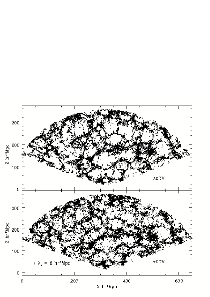
Figure 2: Shown here are the central slices of the $\Lambda$CDM mock SDSS catalogue and of one of the realizations of its $\tau$CDM counterpart. Both the catalogues refer to the same set of random numbers. The coordinates refer to the redshift space positions. The fingers-of-God effect is evident from these slices. The galaxy-distribution is constrained to match the observed 2-point correlation function, and the two slices qualitatively look quite similar. The voids in $\Lambda$CDM are however noted to be much cleaner, and the fingers-of-God effect stronger. The galaxy distributions are smoothed with a gaussian window of size 6 h^-1Mpc. In the left corner of the bottom panel we show the window-size to give a feel for the effective smoothing done around every galaxy.

Figure 2 shows the central slices of the $\Lambda$CDM and one of the realizations of $\tau$CDM mock catalogues, with a similar number of galaxies. These slices refer to the same set of random numbers in the simulations.

3.2 Generating Density Fields

Our analysis will be carried out on a continuous density field sampled on a grid with uniform resolution. Thus, having extracted the volume limited samples, we next present our method of generating continuous density fields for these samples.

As noted in the last subsection, the size of the box enclosing a typical sample is ($\Delta$X, $\Delta$Y, $\Delta$Z)$\simeq$(644, 581, 357) h^-1Mpc. We fit a grid of size 184$\times$166$\times$102 onto this box. The size of the cells, i.e., the resolution, turns out to be 3.5 h^-1Mpc. About 63 per cent of the cells are found to be inside the survey boundaries. We first carry out a Cloud-in-Cell (CIC) smoothing by attaching suitable weights to each of the eight vertices of the cube enclosing the galaxy. This procedure conserves mass. About 25 per cent of the cells inside the survey volume acquire nonzero density after CIC smoothing. As we noted earlier, the mean inter-galactic separation is $\bar{\lambda}\sim\bar{n}^{-1/3}\sim$6 h^-1Mpc $\sim$ 1.71$\times\ell_{g}$, where $\ell_{g}$ is the resolution of the grid. Thus we do expect the CIC-smoothing to leave behind an appreciable fraction of cells with zero density. Ideally, a density field should be continuous, and should be defined over the entire sample volume. To achieve this, we need to smooth the CIC-smoothed density field further. We employ a gaussian window

$$W_{s}({\bf r})={1\over\pi^{3/2}\lambda_{s}^{3}}\exp\left(-{|{\bf r}|^{2}\over\lambda_{s}^{2}}\right)$$ (4)

for this purpose. A gaussian window, being isotropic, effectively smooths the matter distribution within $\lambda_{s}$ h^-1Mpc of the cell. Since the purpose of our present investigation is to quantify the morphology of coherent structures, the smoothing scale $\lambda_{s}$ should not be very large. It should be just enough to connect the neighbouring structures. While Gott et al. (1989) prescribe using $\lambda_{s}\geq$2.5$\ell_{g}$ for such applications , we prefer to work with $\lambda_{s}$=6 h^-1Mpc, which is comparable to the correlation length scale in the system, and reasonably smaller than 2.5$\ell_{g}$. As we shall demonstrate below, the behaviour of MFs is remarkably regular even at this smoothing scale. The lower panel of Figure 2 shows the adopted smoothing scale in the overall distribution to develop a feel for the effective smoothing done with the samples. It is clear from here that the large voids should be practically devoid of matter even after smoothing and should be accessible for morphological analysis at the lowest, sub-zero $\delta$-values, whereas the nearby clusters and superclusters should connect up at a suitable density threshold (corresponding to $\delta$$\sim$1-2, see below). The morphology of these superstructures should be accessible at or near the onset of percolation. In this paper, we shall concentrate on the shapes, sizes and geometry of such superclusters and shall quantify these notions in more detail in Section 6.

Prior to smoothing by a gaussian (or say, a top-hat) window, which requires utilising FFT routines, a suitable mask for the cells outside the survey boundaries has to be assumed. It is also to be noted that smoothing leads to a spill-over of mass from the boundaries of the survey to the outer peripheries. Thus, the mass inside the survey is no longer equal to the mass contained in all galaxies. To conserve mass, we employ the smoothing prescription of Melott & Dominik (1993): we prepare two samples; the first containing the CIC-smoothed density field, with cells outside the survey volume set to zero density, and the second reference grid wherein the cells inside the survey volume are all set to unity, while ones outside the survey boundaries are set to zero. Both density fields are smoothed with the gaussian window (Eq.4) at $\lambda_{s}$ = 6h^-1Mpc . The reference grid helps us correct for the effect of having a smoothing window at the boundaries of the survey. We divide the density values of the first grid, cell-by-cell, by the entries for the density values in the reference grid. We find that this corrects for the spill-over of mass at the boundaries, and we indeed find mass inside the survey volume to conserve to a very good accuracy.

Having elaborated on our method to prepare volume limited samples and to recover the underlying density fields, we now elaborate upon our method of analysis and finally present our results. Before embarking on quntifying the morphology of density fields, we shall study the percolation properties of the samples. This is the subject of the next section.

4 Percolation of the Large Scale Structure

Percolation gives us useful insights into the connectivity of the density fields. Earlier workers (for example, Sahni, Sathyaprakash & Shandarin 1997) have found noticeable correlations between the topological behaviour of density fields and their percolation properties. Density fields showing bubble topology, meatball topology or sponge/network topology have distinct features in the way such fields percolate. The 3-D idealized gaussian random fields (hereafter, GRFs), which often serve as a useful benchmark in the study of large scale structure, percolate at 16 per cent of the overdense/underdense volume filling fraction (Shandarin & Zeldovich, 1989), and those defined on a grid percolate at $\sim$30 per cent volume fraction for a variety of power spectra (Yess & Shandarin, 1996). Overdense regions undergoing gravitational clustering percolate at lower values of the filling fraction as compared to GRF. As a result, the difference between the thresholds of percolation (measured in terms of the volume filling fraction) serves as a useful diagnostic with which to quantify the degree of clustering. Such fields show network topology and are characterised by “clusters” having larger length-scales of coherence. Various workers (e.g., Sheth et al., 2003) also find that the dominant morphology of the superclusters (defined for a field when the percolation sets in) is filamentary. Thus, studying the percolation properties of our present catalogues can help us identify a threshold of density at which to look for realistic structures in our survey volumes.

In the ensuing analysis, our results shall refer to 11 density fields (10 mock catalogues due $\tau$CDM and one due to $\Lambda$CDM) scanned at 50 thresholds (or levels) of density. This sampling is not uniform. Our preliminary analysis shows that overdense regions percolate when the overdense volume fraction $\leq$ 10 per cent of the survey volume. On the other hand the underdense regions or voids percolate when the overdense volume fraction is $\sim$70 per cent. Thus, from a morphological perspective, the volume fractions $\leq$30 per cent and $\geq$70 per cent are interesting for overdense and underdense regions respectively. In the intermediate range, both the overdense and underdense regions percolate, and most of the volume is occupied by the largest cluster and the largest void respectively. So practically very little is gained by studying the structures in the range FF${}_{\rm V}\in$(0.3,0.7), where FF_V, the overdense volume fraction is given by

$$FF_{\rm V}={1\over V_{T}}\int\Theta(\rho-\rho_{\rm TH})d^{3}x.$$ (5)

Here $\Theta(x)$ is the Heaviside Theta function.

$$\Theta(x) = 1~{}~{}~{}x\geq 0$$ (6)

$$= 0~{}~{}~{}x<0.$$

$FF_{\rm V}$ measures the volume-fraction in regions which satisfy the ‘cluster’ criterion $\rho_{\rm cluster}\geq\rho_{\rm TH}$ at a given density threshold $\rho_{\rm TH}$. V_T is the total survey volume. In the following, we use $FF_{\rm V}$ as one of the parameters with which to label density contours. Finally, the ranges FF${}_{\rm V}\leq$0.3 and FF${}_{\rm V}\geq$0.7 each are attributed 23 levels of density, each equi-spaced in FF_V. The intermediate range FF${}_{\rm V}\in$(0.3,0.7) is sampled at four levels all equi-spaced with $\Delta$FF=0.1.

Figure 3: The density contrast and the mass filling fraction FF_M are plotted as functions of FF_V, the volume filling fraction which is treated as an independent parameter. The solid line stands for the $\tau$CDM model and is obtained by averaging over 10 realizations. The dashed line stands for the $\Lambda$CDM model. Please refer to the text for further comments.

In Figure 3 we study the density contrast $\delta$ and the mass filling fraction FF_M with respect to FF_V. The first noticeable effect which the biasing brings in is, that unlike the dark matter simulations (Sheth et al., 2003), FF_M no longer distinguishes the two models. At all the chosen levels, the overdense mass fraction, i.e., the fraction of galaxies enclosed by a given normalised volume FF_V,  is similar in $\Lambda$CDM and $\tau$CDM. The mass-parametrisation which was noted to be so effective in distinguishing dark matter distributions in various models, cannot perform any better than FF_V. We shall return to this issue in Section 6. We further note that, the density contrast $\delta$ follows similar pattern in both the models.

We employ a friends-of-friends (FOF) based cluster-finding code to study the number of clusters and the overdense volume fraction in the largest cluster (FF_LC) at all the 50 density-levels. FF_LC stands for the volume of the largest cluster normalised by the total overdense volume.

For cubic samples, the percolation is said to have set in when the largest cluster first spans across the full length of the box (by periodicity arguments, this is equivalent to having the supercluster spanning across the infinite space). In the case of redshift surveys wherein the matter-distribution generally falls within a cone, we cannot utilise such a convention, for the survey boundaries diverge as we go radially outwards and a supercluster spanning the survey volume could as well be touching the two boundaries nearer to the observer, without visiting other parts of the survey volume. Clearly, this does not mean the system has percolated. Thus, for conic survey volumes, spanning the survey volume is not a robust concept to signify the onset of percolation. Instead, Klypin & Shandarin (1993) motivate utilising the merger property of clusters to define the onset of percolation. Following this convention, we measure the rate of growth of the volume of the largest cluster. The highest rate of growth signifies pronounced merger of clusters, leading to a single, larger cluster. The threshold of density at which the growth-rate is highest is defined to be the percolation threshold.

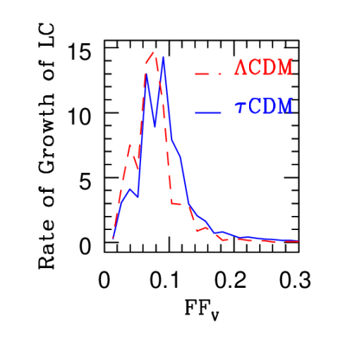
Figure 4: For samples with arbitrary survey geometry, the growth-rate of the volume of the largest cluster is important for quantifying the onset of percolation. Here this quantity is plotted w.r.t. FF_V. The merger activity in $\tau$CDM is pronounced for FF_V$\in$[0.06,0.1]. We take FF${}_{\rm V}\sim$0.08 to be the percolation threshold for this model. Similarly, in case of $\Lambda$CDM, the largest cluster growth is highest at FF${}_{\rm V}\sim$0.08. Hence, we take FF${}_{\rm perc}^{\Lambda}$=0.08. Where needed, we explore the whole range of density levels $\delta$$\in$[$\delta$_perc,$\delta$_max].

Figure 4 shows the rate of growth of the largest cluster as a function of FF_V.  For $\tau$CDM, we use the data after averaging over all 10 mock realizations, and find that the merger rate is highest in the range FF_V$\in$[0.06,0.1]. For our purpose, we take FF_V of 8 per cent to be the percolation threshold for $\tau$CDM model. We find that the largest cluster of $\Lambda$CDM undergoes a pronounced merger at FF_V$\sim$0.8, bringing in 30 per cent of the overdense volume fraction into the largest cluster. (see Figure 5). We have only one realization for the $\Lambda$CDM model, so a statistically robust statement cannot be made, but for all purposes, we treat FF_V= FF${}_{\rm V}^{\rm perc}$=0.08 as the percolation threshold for $\Lambda$CDM. Where needed, we explore the entire range of FF_V$\leq$0.4 for various statistics. To summarise, FF_V${}_{\rm,perc}^{\Lambda}\simeq$FF_V${}_{\rm,perc}^{\tau}$=0.08.

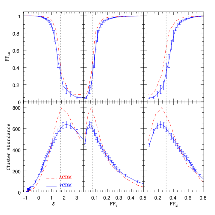
Figure 5: We study here the cluster abundance and FF_LC, the fraction of overdense volume in the largest cluster, with three different parameters, $\delta$, FF_V and FF_M. The $\tau$CDM curves are averaged over 10 realizations. The percolation of the volume of the largest cluster is remarkably similar in both the models. The percolating supercluster occurs at $\delta_{\rm perc}^{\Lambda,\tau}$=1.7 in both $\Lambda$CDM and $\tau$CDM. The dotted vertical lines in all the plots signify the onset of percolation. We also note from the lower panels, that the number of clusters in $\Lambda$CDM are larger than in $\tau$CDM. This could be a useful means to distinguish these two models.

Finally, Figure 5 shows the percolation properties of our samples. We study the cluster abundance (lower panels) and the filling fraction in the largest cluster FF_LC (the upper panels) as functions of three different parameters, $\delta$, FF_V and FF_M. The parameter values corresponding to percolation are marked with a dotted line for both the models. For $\tau$CDM, we again show the curves after averaging over the 10 available realizations. We note that the clusters are slightly over-abundant in $\Lambda$CDM compared to $\tau$CDM. Assuming a similar degree of scatter in the cluster-abundance, we conclude that the Number of Clusters statistic is useful to discriminate the two models. The quantities FF_V^perc are quite closer to each other for both models as we noted earlier (middle, upper panel). From here, we conclude that the spatial connectedness, as measured in terms of percolation of the volume of the LSS alone is not sufficient to distinguish between the two models. The top-right panel does indicate that in $\tau$CDM, 30 per cent of the total mass is in “clusters” when percolation sets in, and 32 per cent of this mass (which amounts to $\sim$22000 galaxies!) is in the percolating supercluster. Looking at the similar volumes that these systems occupy at percolation (although the $\Lambda$CDM percolation sets in a little earlier than in case of $\tau$CDM), clearly other geometric and topological descriptors like Minkowski Functionals would be more insightful to assess the properties of the superclusters. In passing, we note two important aspects of the models: (1) The upper left panel shows that $\delta$ is distributed over the same range of values for both the models. (2) For both the models, $\delta$${}_{\rm perc}\in$[1,2], which coincides with the conventional definition of superclusters. Thus, this range in $\delta$ is in general useful for studying the network of superclusters. We shall make use of this fact in our subsequent analysis.

5 Estimating Minkowski Functionals

The work of Gott, Melott & Dickinson (1986) led to a revival of interest in the paradigm of studying and quantifying the excursion sets of the cosmic density fields; an idea which was successfully propounded earlier in the topological context by Doroshkevich (1970). These early efforts however, were devoted to studying the topology and connectivity of isodensity contours of the large scale structure (hereafter, LSS)(Melott, 1990). It was soon realised that topology alone may not be sufficient to describe LSS, and that it should be complemented with geometrical information pertaining to excursion sets. This goal was met in the form of the Minkowski Functionals (hereafter, MFs)(Mecke, Buchert & Wagner, 1994). A set of grid-based methods (e.g, the Crofton’s formulae, the Koenderink Invariants) and a method to calculate MFs for point processes (the Boolean grain model) were proposed (Mecke, Buchert & Wagner, 1994; Schmalzing & Buchert, 1997) to address the issue of estimating the MFs. (In fact, the CONTOUR3D code to calculate the topology of LSS by Weinberg (1988) is also grid-based.)

Sheth, Sahni, Shandarin & Sathyaprakash (2003) proposed a novel method to calculate MFs by following a mathematically precise prescription with which to construct isodensity contours while quantifying them, as opposed to grid-approximations to contours implicit in earlier treatments. Their method accurately modelled isodensity contours in addition to performing an online calculation of MFs for these contours.

In 3$-$D, the MFs are four in number. The first three of these are geometric in nature, and change when we deform the surface, whereas the fourth is a topological invariant and tells us how many handles does a surface have in access of the holes which it completely encloses. The four MFs are

• [1] Volume $V$ enclosed by the surface,

• [2] Area $S$ of the surface,

• [3] Integrated mean curvature $C$ of the surface,

  $$C=\frac{1}{2}\oint{\left({1\over R_{1}}+{1\over R_{2}}\right)dS},$$ (7)

• [4] Integrated gaussian curvature, or the Euler characteristic,

  $$\chi=\frac{1}{2\pi}\oint{\left({1\over R_{1}R_{2}}\right)dS}.$$ (8)

A related measure of topology is the genus $G=1-\chi/2$, which is what we use in all our analysis.

We shall evaluate MFs for mock catalogues by triangulating isodensity surfaces using SURFGEN. SURFGEN is a fusion of a robust surface modelling scheme and an efficient algorithm to calculate the geometric quantities. The algorithm to calculate MFs on a triangulated surface and the code SURFGEN have been discussed extensively by Sheth et al. (2003) and we refer the reader to that paper for further details. On a dual processor DEC ALPHA machine, SURFGEN calculates the MFs for all the clusters found at about 100 levels of density on a typical 128³ grid in within a few hours’ time. This amounts to probing the MFs for about 100 000 clusters of varying sizes. In fact, in our present application, which involves a grid which is 1.5 times larger than this, the calculations for all the 11 samples could be accomplished in within 2 days’ time. This highlights the scope of using SURFGEN in more ambitious applications involving larger number of realizations studied at higher resolution. Our method of analysis and the results are described in the next section.

6 Geometry, Topology and Morphology of Mock Catalogues

The mock SDSS catalogues being studied here, by construction, have the same two-point correlation function in the range 1 to 10 h^-1Mpc. Since Minkowski Functionals are shown to depend on the entire hierarchy of correlation functions, they may be expected to differentiate between models as similar as $\tau$CDM and $\Lambda$CDM. This will indeed be the case, as we shall show below.

One of the fascinating aspects of the LSS is related to its visual impression. The LSS as revealed in various dark matter simulations and redshift survey slices reveals a cosmic web of interconnected filaments running across the sample, separated by large, almost empty regions, called voids (see Figure 2 for an illustration). Our study will focus both on global MFs which characterise the full excursion sets of the cosmic density field and partial MFs which, together with Shapefinders, help us study the shapes and sizes of the structural elements (superclusters) of the cosmic web .

We begin by first studying the global Minkowski functionals. Next we focus on how the largest cluster evolves with the volume fraction. The last two subsections deal with the morphology of individual superclusters in $\tau$CDM and $\Lambda$CDM models.

6.1 Global Minkowski Functionals

As mentioned earlier, we sample the 11 density fields (1 $\Lambda$CDM + 10 $\tau$CDM) at 50 levels of density. The criteria adopted for their choice has been described earlier (see Section 4). The levels uniformly correspond to the same set of volume fractions FF_V,  for all the samples, which makes comparison between models easier.

We find clusters using the friends-of-friends (FOF) algorithm based Clusterfinder code at every level of density. Next we run SURFGEN on all the clusters and estimate their MFs by modelling their surfaces. These are the partial MFs and are useful for studying the morphology of individual clusters. We use the additivity property of the MFs and evaluate global MFs by summing over the contribution of partial MFs due to all the clusters at a given level of density. For $\tau$CDM, we use the measurements from available 10 realizations to produce average global MFs.

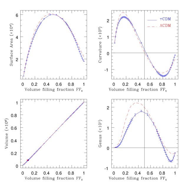
Figure 6: Global Minkowski functionals are evaluated at 50 density levels at a common set of volume filling fractions and are studied here w.r.t. FF_V. We show the values of global MFs as normalised to the volume of [100 h^-1Mpc]³.  The global MFs for $\tau$CDM model are averaged over the available 10 realizations (solid lines) and the errorbars represent 1$\sigma$ deviation. Assuming the same level of accuracy for $\Lambda$CDM, we may conclude that the global MFs with volume parametrisation can indeed clearly distinguish $\tau$CDM from $\Lambda$CDM. Considering the fact that all the samples show the same two$-$point correlation function, the above difference can be attributed to the higher order correlation functions. MFs are able to respond to such a difference, and hence can be taken to be robust measures for quantifying the cosmic web. For further discussion, please refer to the text.

Figure 6 shows the dependence of the global MFs on the volume fraction FF_V.  The solid curves represent the mean global MFs due to $\tau$CDM model and the error-bars stand for the 1$\sigma$ standard deviation. The dashed curves stand for the $\Lambda$CDM model . First, we note that the global MFs of the $\tau$CDM model are extremely well constrained. This shows the remarkable accuracy with which SURFGEN will enable us to measure the MFs of the LSS due to large datasets like SDSS and 2dFGRS. We further note that the two models can be distinguished from each other with sufficient confidence using the global area, mean curvature and genus measurements at FF_V$\leq$0.5 , whereas the global volume scales linearly with FF_V,  as expected. Distinctly different trends of MFs in two models are due to the contribution of the higher order correlation functions, and do indeed reflect the manner in which the galaxies cluster in $\Lambda$CDM as against $\tau$CDM. This can be dubbed to be the success of MFs as robust statistics ideal for quantifying the cosmic web.

From the dynamical point of view, these results carry some surprises. As noted by Melott (1990); Springel et al. (1998), the amplitude of the genus-curve drops as the N$-$body system develops phase correlations. Given two density fields, the system with larger genus-amplitude shows many more tunnels/voids which are, therefore, smaller in size. As time progresses, the voids are expected to expand and merge, leading to a drop in the genus-amplitude, while the phase correlations continue to grow. With this simple model, one could correlate the amount of clustering with the relative smallness of the amplitude of genus, and therefore, of the area and the mean curvature. As illustrated by Sheth et al. (2003), the dark matter distribution of $\tau$CDM model due to Virgo group consistently shows considerably larger amplitudes for the MFs compared to the $\Lambda$CDM model , whereas, we find the reverse trend in the MFs of “the galaxy distributions” due to the same two models. This is a sufficiently robust result because, the $\tau$CDM curves are averaged over 10 realizations. We could interpret this as an instance of the phase-mismatch between the galaxy-distribution and the underlying dark matter distribution and could attribute it to the biasing prescription invoked. This is supported by the fact that CHWF require large anti-bias in high density regions of the $\Lambda$CDM model.

To conclude, the study of the global MFs reveals from here that, local, density-dependent bias could lead to an apparent phase-mismatch or different phase-correlations among the dark matter and the galaxies. In passing, we also note that $\Lambda$CDM preserves its unique bubble shift which is pronounced compared to $\tau$CDM (lower right panel of Figure 6).

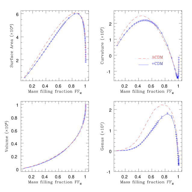
Figure 7: Global Minkowski functionals are studied here w.r.t. FF_M,  which is defined as the overdense mass fraction. The MF-values are normalised to a volume of [100 h^-1Mpc]³. In addition to the fact that the models can be distinguished, we also note that the geometry and topology of the excursion sets, when coupled with the overdense mass fraction, is markedly different in both the models at and beyond the onset of percolation.

Figure 7 shows the global MFs plotted against the overdense mass-fraction FF_M.  The mass-volume relation is remarkably similar among both the models. This again is an effect of biasing. In addition to the fact that the models can be distinguished, we also note that the excursion sets enclosing the same fraction of mass due to the two models show appreciably different geometry and topology. Thus, assessing the excursion sets enclosing the same mass-fraction could be a useful means of analysing the realistic data and comparing them with the mock data.

6.2 Minkowski Functionals for the Largest Cluster

As we scan the density fields by lowering the density threshold, the largest cluster of the system grows in size due to merger of smaller clusters. The manner of evolution of the largest cluster is connected with the percolation properties of the system. We noted earlier (Section 4) that the largest cluster spans most of the volume by the time the volume fraction reaches FF_V$\sim$0.3. In fact, most of the features in the global MFs beyond FF_V=0.3 pertain to the evolution of the largest cluster alone. Hence, in this section, we study the evolution of the MFs of the largest cluster for FF_V$\leq$0.3. We find that, of the four MFs, the integrated mean curvature (hereafter, IMC) and the genus are the best discriminants. Further, it is instructive to see the behaviour of the largest cluster with FF_M$-$parametrisation. In Figure 8, we show the IMC and genus for the largest cluster as functions of FF_V (left panels) and FF_M (right panels).

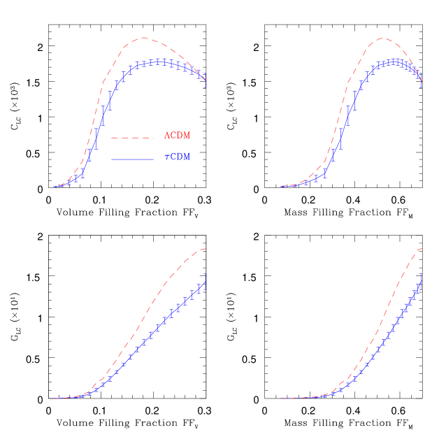
Figure 8: The largest cluster spans most of the sample-volume for FF_V$>$0.3. Here we study the dependence of the mean curvature and genus of the largest cluster of $\tau$CDM and $\Lambda$CDM w.r.t. FF_V (left panels) and FF_M (right panels). Note the well-constrained behaviour of both the measures for $\tau$CDM, and the distinctly different trend observed for them in $\Lambda$CDM. Please refer to the text for the discussion.

We notice in the bottom-left panel of this figure that the genus of the largest cluster remains vanishingly small until the onset of percolation in both the models. However, once percolation sets in, the genus of the largest cluster grows much more rapidly in $\Lambda$CDM than in $\tau$CDM. The larger genus is indicative of greater number of tunnels (more porosity) which the $\Lambda$CDM structure exhibits relative to its $\tau$CDM counterpart. While the genus in case of $\tau$CDM seems extremely well-constrained (small scatter), the fluctuations in IMC, at least at smaller FF_V$-$values ($<$0.15), are reasonably large. This could be inferred as fluctuation in the sizes of the tunnels forming due to the merger of the smaller clusters, while their total number conserves for a given FF_V.  The IMC and genus of the largest cluster in the range FF_V$\in$[0.05,0.3] could be some of the best discriminants of the two models.

6.3 Morphology of the Superclusters

This and the following subsection are devoted to a critical study of the morphology of the ensemble of superclusters. Based on a statistical study of many realizations of $\tau$CDM, we are able to establish it for the first time that the supercluster shapes and their sizes are very well constrained measures, suitable as ideal diagnostics of the large scale structure of the Universe and are sensitive to the cosmological parameters of the model(s).

Since we are dealing with density fields, our superclusters are defined as connected, overdense objects. In Section 4, we studied the percolation properties of the density fields and found that the percolation takes place at a threshold of density corresponding to $\delta$=1.7 in both $\Lambda$CDM and $\tau$CDM. Further, $\delta$${}_{\rm max}\simeq$ 3.5. Thus at the highest threshold of density, we are still within the weakly nonlinear regime, and may find sufficiently large connected objects which might act as dense progenitors of the percolating superclusters. With this anticipation, we find it advisable to study the morphology of the ensemble of superclusters as a function of the density contrast over the entire range $\delta$$\in$[0,$\delta$_max]. In so doing, we are also able to assess how the morphology of the LSS changes with the density-level.

The morphology of the superclusters is quantified in terms of a set of Shapefinders (Sahni, Sathyaprakash & Shandarin, 1998; Sheth et al., 2003). The dimensional Shapefinders have dimensions of length and are given by

$$T={3V\over S};~{}~{}~{}B={S\over C};~{}~{}~{}L={C\over 4\pi(G+1)}.$$ (9)

For objects with fairly simple topology, the above Shapefinders give us a feel for the typical thickness (T), breadth (B) and length (L) of the object being studied. Since we have demonstrated that most of the superclusters are simply connected objects near or before the onset of percolation, this interpretation is valid for structures defined in this regime. Further, a combination of (T,B,L) can be used to define Planarity (P) and filamentarity (F) of the object.

$$P={B-T\over B+T};~{}~{}~{}F={L-B\over L+B}.$$ (10)

Individual superclusters in a given realization of, say, $\tau$CDM may follow a distribution of shapes and sizes, not necessarily coinciding with a similar list due to another realization. Hence, to make a statistical study of a given model, we average over the shapes of individual superclusters defined at a given threshold of density, and test whether the average morphology as a function of the density-level is well constrained. For this purpose, we use the volume and mass averaged Shapefinders defined as follows.

$$\bar{P}_{V,M}(\delta_{\rm th}) = {\sum_{i=1}^{N_{C}}{Q_{i}\times P_{i}}\over\sum_{i=1}^{N_{C}}Q_{i}}$$

$$\bar{F}_{V,M}(\delta_{\rm th}) = {\sum_{i=1}^{N_{C}}{Q_{i}\times F_{i}}\over\sum_{i=1}^{N_{C}}Q_{i}},$$ (11)

where the quantity $Q_{i}$ may refer to the mass or volume of the i^th supercluster defined at the level $\delta$_th, and the summation is over all the objects. It is to be noted here that the average planarity and filamentarity are mostly contributed by the structures with large volume and/or mass. There are a finite number of such objects before the onset of percolation. Hence, in this regime, we probe the average shape of these objects. However, once the percolation sets in, the average morphology mainly reflects the morphology of the largest object in the system.

We evaluate $\bar{P}_{V,M}$ and $\bar{F}_{V,M}$ for all the 11 samples at the density levels corresponding to $\delta$$\in$[0,$\delta$_max]. The measurements due to 10 $\tau$CDM realizations are used for averaging and for evaluating the errors.

Figure 9: The dimensionless Shapefinders (P,F) are evaluated for all the clusters at a given density level $\delta$_th. These Shapefinders are volume-averaged and are studied w.r.t. FF_V (left panels). They are also mass-averaged and are studied w.r.t. FF_M (right panels). The average shape of the cosmic web assumes increasingly planar morphology as $\delta$_th is lowered. The corresponding negative filamentarity is due to the presence of large voids which lead to the development of appreciable negative curvature in the system. The average filamentarity in the system is highest near the onset of percolation, thus making it ideal for the study of structures which are evident in the visual impression of the cosmic web. The average morphology revealed in terms of $\bar{P}_{V,M}$ and $\bar{F}_{V,M}$ is extremely well constrained for a given model and could be a useful diagnostic for discriminating the models of structure formation.

Figure 9 shows $\bar{P}_{V,M}$ and $\bar{F}_{V,M}$ studied as functions of FF_V (left panels) and FF_M (right panels) respectively. The solid lines refer to $\tau$CDM and the dashed lines refer to $\Lambda$CDM. The vertical bars stand for the 1$\sigma$ errors. We observe that

• $\bar{P}_{V,M}$ and $\bar{F}_{V,M}$ are well constrained statistics and hence, can be used to reliably assess the morphology of the LSS.

• The average planarity of the LSS steadily increases as we lower the threshold of density.

• The average filamentarity initially increases, reaches a maximum where the percolation sets in, but drops to sub-zero values after FF_V$\sim$0.18.

This implies that the square of the area of the excursion set is always greater than thrice the product of the volume and curvature. Further, C² is superseded by 4$\pi$(G+1)S at FF_V$>$0.18. A steady drop in the curvature is responsible for this behaviour. We note that the system also tends to become increasingly spongy. Taken together, these observations lead to the following picture: as the density level is brought down, the overdense structures connect up across the sample-volume. This at a time leads to large scale filaments and also to the birth of large voids in the system, signifying the onset of percolation. As revealed in the top panels, the filamentarity of the system is highest at the time. With a further drop in $\delta$, the filaments surrounding the “voids” grow thicker and locally these assume a slab-like structure. Such an excursion set, at a time has large planarity, but also has large negative curvature due to being surrounded by large, almost spherical voids. This negative curvature is responsible for the large negative filamentarity .

We notice that both the statistics are extremely well-constrained. Further, $\bar{P}_{V,M}^{\Lambda}\geq\bar{P}_{V,M}^{\tau}$ and $\bar{F}_{V,M}^{\tau}\geq\bar{F}_{V,M}^{\Lambda}$. This feature can be used to distinguish these two models, and is an instance of the fact that morphology of LSS is an equally robust statistic as MFs to compare LSS due to rival models of structure formation.

We finally note that the superclusters defined according to the conventional definition ($\delta$${}_{SC}\in$[1,2]) do correspond to the percolating structures in the system, and indeed exhibit the highest filamentarity (the top panels of Figure 9). This proves that the Shapefinder statistics conform to our visual impression while quantifying the LSS. In the next subsection, we shall try to quantitatively asses the sizes of these superclusters and shall demonstrate that these measures are sensitive to the models being investigated, enabling us to distinguish the two models successfully.

6.4 Cumulative Probability Functions

In this subsection we make a quantitative investigation of the sizes of the superclusters and study the variation of these measures as functions of the density contrast. Our main focus is to make a statistical study of these measures and to develop a methodology to handle various statistics due to many realizations of a given model. We also compare the sizes of superclusters in $\tau$CDM with those in $\Lambda$CDM and find that these are sensitive to the model being investigated and can be used to distinguish the two models.

For reasons explained earlier, we find it advisable to carry out the exercise over a set of levels of density. We study the sizes of superclusters starting from the highest density level ($\delta$$\simeq$3.5) down to the percolation threshold.

Since the sizes of individual structures may vary from one realization to another, it is not meaningful to prepare a list of, say, top N superclusters in a given realization and check its statistical significance over other realizations. There may not be any unique correspondence of the rank of the supercluster in the list and its size. This is mainly because at the density-levels above or near the percolation threshold, there may be many structures with comparable sizes and masses. So the sorted array of structures in this range of density-levels will show a large amount of Poisson fluctuations in the size of, say, the i^th largest cluster. Hence, a more meaningful approach is to study the cumulative probability functions of the Shapefinders so as to know how many superclusters in a given ensemble of them, have their sizes greater than a given triplet (T,B,L).

As noted in Section 4, all the 10 samples of $\tau$CDM being studied here have comparable number of clusters at any given threshold of density, and that these are only marginally smaller in number than in $\Lambda$CDM. Further, we found that the global geometry and topology of the $\tau$CDM density fields is extremely well constrained. Hence, it is justified to construct cumulative probability functions (hereafter, CPFs) of various quantities using an ensemble which contains the clusters due to all the 10 realizations of $\tau$CDM . The CPF of a given quantity Q is a fraction of the total number of structures having the value of Q greater than a chosen value q. In our case, the total number of clusters amounts to the sum over all the realizations of $\tau$CDM and is close to a few thousand. It turns out that it is beneficial to work with such large number of clusters, so that we have sufficient number of structures which are otherwise rare in a given sample. By finding these in sufficient number in a bigger ensemble, we can put an upper limit on the sizes of superclusters at any given threshold of density, without hampering our conclusions by Poisson noise.

To begin with, we study the CPFs of the dimensional Shapefinders, the so called, Thickness (T), Breadth (B) and Length (L) of the superclusters with FF_V as a parameter.

Figure 10: The CPFs of dimensional Shapefinders are studied as functions of the density level for $\tau$CDM. The bottom panel shows the associated volume filling fractions. The percolation curves are shown as bold, solid lines. We notice that the clusters grow thicker, broader and longer as we increase the volume fraction (at any given triplet (T,B,L), there are more number of them thicker than T, broader than B and longer than L as we decrease $\delta$).

Figure 10 shows the results. We notice that the CPFs follow a specific pattern of evolution. While a typical range of thickness and breadth of the structures is fixed (T $\in$(0,13) h^-1Mpc and B $\in$ (0,17) h^-1Mpc), the fraction of clusters with a given thickness and breadth increases with increasing FF_V. Thus, the structures become thicker and broader as we lower the threshold, as anticipated. The CPF of length, on the other hand, extends to high L$-$values upon increasing FF_V. This implies that the longer structures become statistically more significant with the decrease of $\delta$, while their thickness and breadth increases only marginally. Thus, as $\delta$$\rightarrow$$\delta$_perc, the filamentarity of the individual superclusters should increase. At the highest thresholds, however, the superclusters might look only marginally filamentary (F$\sim$0.25, P$\sim$0.1) (see, Figure 9), and in realistic situation, may give us an impression of being more like ribbons. . We infer that the top 10 superclusters in $\tau$CDM should have their length $\geq$40 h^-1Mpc at $\delta$$\sim$$\delta$_max, and these should grow to become as long as L$\geq$90h^-1Mpc at the onset of percolation. The longest superclusters at percolation, which are necessarily rare (say, a few in 1000), might be as long as 150h^-1Mpc.

To summarise, the supercluster-sizes are dependent on the threshold of density at which the superclusters are defined. Based on the study of CPFs as functions of $\delta$_th we infer that the thickness and breadth of the structures are comparable to one another at all thresholds of density $\delta$$\leq$$\delta$_perc, with breadth B always slightly higher than thickness T. We have noted that at percolation, the largest superclusters could be as long as 150 h^-1Mpc, and the superclusters with length L$\in$[90,150] h^-1Mpc are relatively more frequently to be found (say, with a few per cent probability in an ensemble of 1000 structures).

We are limited by the availability of only one realization of $\Lambda$CDM. Hence similar conclusions cannot be reliably drawn for this model, but a study of CPFs of $\Lambda$CDM superclusters does reveal similar trends.

In order to see whether the supercluster sizes and their morphology can be utilised to distinguish the two models, we studied the CPFs of T, B and L due to $\Lambda$CDM and $\tau$CDM together.

Figure 11: The cumulative probability functions for thickness (T), breadth (B) and planarity (P) are shown for both the models at three thresholds of density. The fraction of clusters with a given thickness or breadth in $\tau$CDM are always greater than or equal to the fraction of clusters in $\Lambda$CDM. Further CPF^Λ(P)$\geq$CPF^τ(P). These Shapefinders can hence, be used to distinguish these models.

We find that near to the onset of percolation, the two dimensional Shapefinders thickness and breadth, and the planarity of the superclusters do give a detectable signal. Figure 11 shows the results. The thick solid lines refer to $\tau$CDM. The 1$\sigma$ error-bars are computed assuming a Poisson statistics and go as the square-root of the number of clusters available at a given value of (T,B,P). It has been checked that the CPFs due to individual realizations fall within 1$\sigma$ of the CPFs due to the total ensemble in most cases. Thus our decision to use the total ensemble (cumulative of all the clusters and due to all the realizations) and of assuming Poisson errors is justified. To make the comparison ideal, we choose to incorporate Poisson errors on the CPFs of the only available realization of $\Lambda$CDM as well. As shown in the figure, the $\tau$CDM CPFs of thickness and breadth are systematically higher than those of $\Lambda$CDM at FF_V=9.1, 10.4 and 11.7 per cent. Thus, we are able to establish that the $\tau$CDM superclusters with a given thickness are statistically larger in number than in $\Lambda$CDM. Assuming similar number of clusters in the two models, we could infer that the $\tau$CDM superclusters are thicker than those in $\Lambda$CDM. This effect is pronounced enough to be detected with a set of limited number of realizations. The topmost panels further reveal that CPF^τ(P)$\leq$CPF^Λ(P). We conclude from here that the thickness, breadth and planarity of superclusters follow well-defined distributions which are special to the model being studied.

Figure 12: Shown here are the cumulative probability functions of length L for clusters of $\tau$CDM and $\Lambda$CDM at two thresholds of density corresponding to FF_V=7.8 per cent (just before the onset of percolation) and FF_V=11.4 per cent (after the onset of percolation). We find the CPFs of the two models to be distinctly different at longer length-scales. The dashed line refers to the CPFs due to the first realization of $\tau$CDM which shares the initial set of random numbers with $\Lambda$CDM. The largest superclusters of $\tau$CDM are systematically larger than those due to $\Lambda$CDM.

In order to test whether we can constrain the length of superclusters of a given model, we studied the CPF for length L, following identical procedure. Figure 12 shows the results, where the CPF(L) have been evaluated at FF_V=7.8 per cent (at the onset of percolation) and at FF_V=11.7 per cent (after the percolation). We notice that at the onset of percolation, the length of the longest $\tau$CDM superclusters could be as large as 90 h^-1Mpc, whereas their $\Lambda$CDM counterpart structures, which exhibit same degree of statistical significance, are relatively shorter with L${}_{\rm max}\geq$ 55 h^-1Mpc. We conclude that the $\tau$CDM superclusters tend to be statistically longer than their $\Lambda$CDM counterpart structures. Thus, we can also utilise the length of the superclusters to compare and distinguish the two models. After the percolation, the longest structure dominates the survey volume and enters only as a Poisson fluctuation in the CPF of length. The remaining structures are evidently shorter in length compared to their longer progenitors at percolation, so that CPF(L) are confined to lower values of L. This effect is evident in the right panel of Figure 12. In both the panels, shown as dashed line is the CPF(L) due to the first realization of $\tau$CDM which shares its set of initial random numbers with the $\Lambda$CDM simulation. We note the sharp tendency of $\tau$CDM structures to be longer than those of $\Lambda$CDM, an effect which successfully enables us to distinguish the two models of structure formation.

7 Discussion and Conclusions

This paper provides a theoretical framework and a methodology to analyse the galaxy-distribution revealed by large 3-dimensional redshift surveys. The exercise is in the wake of preparing to tackle the redshift surveys like 2dFGRS and SDSS, and consists in studying the geometry, topology and morphology of the LSS as revealed by the volume limited samples derived from 10 realizations of mock $\tau$CDM$-$based SDSS catalogue. These volume limited samples are prepared so as to refer to the same physical volume, and exhibit similar number density of galaxies. The density fields used in our calculations are prepared after smoothing all the samples at 6 h^-1Mpc.

We use SURFGEN (Sheth et al.2003) for calculating MFs, and find MFs as well as the derived morphological statistics, the Shapefinders, to be well-constrained statistics, useful to probe the contribution of the higher order correlation functions on the clustering of the galaxy-distribution. For this purpose, we compare the measured MFs due to 10 realizations of $\tau$CDM with those due to a realization of $\Lambda$CDM. All the 11 realizations, by construction, reproduce the observed two$-$point correlation function measured using the APM catalogue, and show similar clustering amplitude. Some of the important results of our analysis are summarised below:

• We show that the global MFs (defined as the sum of partial MFs over the set of all the clusters at a given threshold of density) of $\tau$CDM show systematically lower amplitude compared to those due to $\Lambda$CDM, an effect which enables us to distinguish the two models, and can be attributed to the nonzero higher order correlation functions. Considering the fact that higher order correlation functions are cumbersome to estimate and offer little insight in their interpretation, this can be termed as a success of MFs as efficient quantifying statistics of LSS.

• The Virgo simulations of dark matter showed higher amplitude of MFs for $\tau$CDM compared to $\Lambda$CDM (see Sheth et al.2003). The cosmological parameters used by Virgo group match with those employed by CHWF except for the shape parameter $\Gamma$, which is 0.21 in the former case and 0.25 in the latter. We assume that this minute difference in $\Gamma$ will not alter the above trend so long as both the models start with the same power spectrum. The galaxy distributions due to both the models were analysed in this paper, and we found a reversal in the above trend: The MF-amplitudes for $\tau$CDM were found to be smaller than $\Lambda$CDM.

  We note that the relative smallness of the amplitudes of MFs reflects the higher degree of phase correlations in the matter-distribution. Taken together with this fact, our above observation points out that scale-dependent biasing could lead to an apparent phase-mismatch between the galaxy-distribution and the underlying matter-distribution. Thus, there may be larger degree of phase-correlations in the matter-distribution of $\Lambda$CDM compared to $\tau$CDM, but the biased galaxy-distribution of $\Lambda$CDM would appear to exhibit smaller phase-correlations compared to $\tau$CDM. We note however, that these results are affected by the constraint that the bias is fixed so as to reproduce the observed 2$-$point correlation function (see Section 2).

  An analysis of 2dFGRS performed by Lahav et al. (2002) concluded that the average bias on scales 0.02 $\leq k\leq$ 0.15 h Mpc^-1 is indeed $\sim$1 . In light of the above fact, it will be interesting to see how the geometry, topology and morphology of the LSS change in the presence of scale-independent, constant bias. From our analysis, however, it is clear that bias in various structure formation scenarios can play important role, and comparing the dark matter distributions with the SDSS and/or 2dFGRS galaxy distributions is not an advisable way of testing the model(s) of structure formation against the observations. A realistic treatment of bias en route the proper treatment of the physics of galaxy formation in preparing a mock catalogue, is desired in any such exercise.

• Since we had access to 10 realizations of $\tau$CDM, we made a statistical study of the shapes and sizes of the superclusters occurring in this model. We found the thickness and breadth of the superclusters to increase only marginally over a range of $\delta$ (T, B$\in$[1,17]h^-1Mpc; T$\leq$B). However, the length of the largest superclusters increases monotonically from $\sim$40 h^-1Mpc to $\sim$90 h^-1Mpc as $\delta$$\rightarrow$$\delta$_perc. Near the percolation, the $\tau$CDM superclusters with length $\geq$90 h^-1Mpc are $\sim$ 1 per cent probable to be found (say, the top 10 in an ensemble of 1000 structures). However, the longest (and necessarily the most massive) superclusters could be as long as 150 h^-1Mpc and are rare to be found, with less than 1 per cent probability in a volume as big as that covered in this analysis. These findings are to be confronted with recent observational work by Brand et al. (2003) who report rare structures of the size of $\sim$100 Mpc being traced by radio galaxies. The dominant morphology of the superclusters is prolate, or ribbon-like at the highest threshold of density, and it evolves to become more filamentary as the threshold is lowered toward the percolation threshold.

• We further found that the CPFs of thickness and breadth near the percolation threshold show distinctly higher amplitude in $\tau$CDM compared to $\Lambda$CDM. Even planarity of the two models shows appreciably different distribution for the two models. These Shapefinders, thus, could be good discriminants of the structure formation scenarios.

• A study similar to the above, repeated for the length of the superclusters reveals that the longest superclusters of $\tau$CDM are likely to be longer than their $\Lambda$CDM counterpart structures at the same level of significance. In particular, whereas the longest superclusters of $\tau$CDM could be as long as 90 h^-1Mpc, the $\Lambda$CDM superclusters have L$\geq$55 h^-1Mpc.

To summarise, we have established that the Minkowski Functionals estimated using SURFGEN are well constrained statistics and can be reliably used to quantify the geometry and topology of the LSS in various scenarios of structure formation. We have used these to distinguish two rival models of structure formation, namely $\Lambda$CDM and $\tau$CDM, and have explored a set of related measures and morphological statistics like Shapefinders to make such a comparison more robust. We have further measured and reported the sizes and shapes of the superclusters in $\tau$CDM, with a scope of extending similar methodology to other models with the availability of larger number of realizations for them.

Our present exercise does have its limitations, which are mentioned below.

• The effect of redshift space distortions has not been incorporated in the present exercise. We have throughout worked in the redshift space and have not quantified the fingers-of-God effect. Such a treatment is beyond the scope of this paper and shall be taken up in a future work.

• The mock catalogues studied in this paper are prepared by implementing ad-hoc biasing schemes. Although the methodology of analysis is clearly laid out in the present work, a more realistic comparison of the mock data with the observed LSS of the Universe should be carried out using the mock catalogues prepared by incorporating the physics of galaxy-formation in as much detail as possible. The semi-analytic methods, the SPH simulations of galaxy formation and the Conditional Luminosity Function based approach should be able to deliver such mock catalogues in near future.

We hope to address some of the issues mentioned above and extend this work to a comparison of the mock catalogues with the LSS revealed by 2dFGRS and SDSS in near future.

8 Acknowledgements

JVS wishes to thank Varun Sahni for his constant support, encouragement and for his critical comments on the manuscript. Thanks are due to Sergei Shandarin for his encouragement and for the numerous discussions with him from which the author has benifited a lot. It is a pleasure to recall stimulating discussions with Somnath Bharadwaj, Ranjeev Misra and K.Subramanian. JVS also wishes to thank the CHWF team for making the mock data public, and in particular, Shaun Cole who has, time and again, provided useful information pertaining to data in the course of this work. Thanks are due to Matteo Frigo and Steven Johnson for making FFTW public. JVS is supported by the Senior Research Fellowship of the Council of Scientific and Industrial Research (CSIR), India. The data analysed in this paper are available at http://star-www.dur.ac.uk/$\sim$cole/mocks/main.html .

References

- Abazajian et al. (2003) Abazajian, K., Adelman-McCarthy, J.K., Agueros, M.A., Allam, S.S. & the SDSS Collaboration, 2003, astro-ph/0305492
- Basilakos (2003) Basilakos,S. 2003, astro-ph/0302596, Accepted for publication in MNRAS
- Baugh (1996) Baugh,C.M., 1996, MNRAS, 280, 267
- Baugh & Efstathiou (1993) Baugh,C.M., Efstathiou, G., 1993, MNRAS, 270, 183
- Bennett et al. (2003) Bennett, C.L., et al., 2003, ApJS, 148, 1
- Benson et al. (2002) Benson, A.J., Lacey, C.G., Baugh, C.M., Cole, S., Frenk, C.S., 2002a, MNRAS, 333, 156
- Berlind et al. (2003) Berlind,A., Weinberg, D.H., Benson, A.J., et al., astro-ph/0212357
- Bharadwaj, et. al. (2000) Bharadwaj, S., Sahni, V., Sathyaprakash, B.S., Shandarin, S.F., and Yess, C., 2000, ApJ, 528, 21.
- Blanton et. al. (2003) Blanton, M., Hogg, D., Bahcall, N., 2003, ApJ, 592, 819
- Bond & Efstathiou (1991) Bond, J.R. and Efstathiou, G., 1991, Phys.Lett.B, 265, 245
- Brainerd & Specian (2003) Brainerd, T. & Specian, M., 2003, ApJL, 593, 7
- Brand et al. (2003) Brand, K., Rawlings, S., Hill, G., Lacy, M., Mitchell, E., & Tufts, J., 2003, MNRAS, 344, 283
- Couchman (1991) Couchman, H. M. P., 1991, ApJ, 368, 23
- Cole, Hatton, Weinberg, & Frenk (1998) Cole, S., Hatton, S., Weinberg, D.H., Frenk, C.S., 1998, MNRAS, 945
- Cole et al. (2000) Cole, S., Lacey, C.G., Baugh, C.M., Frenk, C.S., 2000, MNRAS, 319, 168
- Colless et al. (2003) Colless, M. and the 2dFGRS team, astro-ph/0306581
- Colley et al. (2000) Colley, W.N., Gott, J. R. III, Weinberg, D. H., Park,C. and Berlind, A. A., 2000, ApJ, 529, 795
- Doroshkevich et al. (2003) Doroshkevich, A., Tucker, D.L., Allam, S. & Way, M.J., astro-ph/0307233, Submitted to Astronomy & Astrophysics
- Einasto et al. (2003) Einasto, J., H”utsi, G., Einasto, M. et al., 2003, Astronomy & Astrophysics, 405, 425
- Fairall (1998) Fairall, A., 1998, Large-Scale Structure in the Universe, John-Wiley & Sons in association with Praxis Publishing, Chichester
- Gott, Melott & Dickinson (1986) Gott, J.R., Melott, A.L. & Dickinson, M., 1986, ApJ, 306, 341
- Gott et al. (1989) Gott, J.R., Miller, J., Thuan, T. X., et al., 1989, ApJ, 340, 625
- Hamilton et al. (1991) Hamilton, A.J.S., Kumar, P., Lu, E., Matthews, A., 1991, ApJL, 374, 1
- Hikage et al. (2003) Hikage,C. Schmalzing, J., Buchert, T., Suto, Y., Kayo, I., Taruya,A., Vogeley, M., Hoyle, F., Gott, J. R. III, Brinkmann, J. et al., astro-ph/0304455, Accepted for publication in PASJ
- Hikage, Taruya & Suto (2003) Hikage, C., Taruya, A.& Suto, Y., 2003, PASJ, 55, 335
- Jenkins et al. (1998) Jenkins, A.R. et al. (for the Virgo Constortium), 1998, ApJ, 499, 20
- Klypin & Shandarin (1993) Klypin, A.A. & Shandarin, S.F., 1993, ApJ, 413, 48
- Kneib et al. (2003) Kneib, J-P., Hudelot, P., Ellis, R., et al., astro-ph/0307299, accepted for publication in ApJ
- Kravtsov et al. (2003) Kravtsov, A.V., Berlind, A., Wechsler, R. et al., 2003, astro-ph/0308519
- Lahav et al. (2002) Lahav, O., Bridle, S., Percival, W.J., et al. and the 2dFGRS team, 2002, MNRAS, 333, 961
- Lahav & Suto (2003) Lahav, O. & Suto, Y., astro-ph/0310642, invited review article submitted to Living Reviews in Relativity
- Magliocchetti & Porciani (2003) Magliocchetti, M. & Porciani, C., 2003, astro-ph/0304003, Accepted for publication in MNRAS
- Martinez&Saar (2002) Martinez, V. & Saar, E., 2002, Chapman & Hall/CRC
- Matsubara (2003) Matsubara, T., 2003, ApJ, 584, 1
- Mecke, Buchert & Wagner (1994) Mecke, K.R., Buchert, T. & Wagner, H., 1994, AA, 288, 697
- Melott (1990) Melott, A.L., 1990, Phys. Rep., 193, 1
- Melott & Dominik (1993) Melott, A.L. & Dominik, K., ApJL, 86, 1
- Norberg et al. (2002a) Norberg, P.,Cole, S., Baugh, C.M. and the 2dFGRS team, 2002a, MNRAS, 336, 907
- Norberg et al. (2002b) Norberg, P., Baugh, C.M., Hawkins, E., and the 2dFGRS team, 2002b, MNRAS, 332, 827
- Peacock & Dodds (1994) Peacock, J. A. and Dodds, S. J., 1994, MNRAS, 267, 1020
- Sahni & Coles, (1995) Sahni, V. and Coles, P., 1995, Phys.Rep., 262, 1
- Sahni, Sathyaprakash & Shandarin (1997) Sahni, V., Sathyaprakash, B.S. & Shandarin, S.F., 1997, ApJL, 476, L1
- Sahni, Sathyaprakash & Shandarin (1998) Sahni, V., Sathyaprakash, B.S. & Shandarin, S.F., 1998, ApJL, 495, L5
- Sathyaprakash, Sahni & Shandarin (1998) Sathyaprakash, B.S., Sahni, V. & Shandarin, S.F., 1998, ApJ, 508, 551
- Sathyaprakash, Sahni & Shandarin (1996) Sathyaprakash, B.S., Sahni, V. & Shandarin, S.F., 1996, ApJL, 462, L5
- Schmalzing (1999) Schmalzing,J., PhD Thesis, Ludwig-Maxmilians-Universitat Munchen
- Schmalzing & Buchert (1997) Schmalzing, J. & Buchert, T., 1997, ApJL, 482, L1
- (48) Schmalzing, J., Buchert, T., Melott, A.L., Sahni, V., Sathyaprakash, B.S. and Shandarin, S.F., 1999, ApJ, 526, 568.
- Shandarin & Zeldovich (1983) Shandarin, S.F. & Zeldovich, Ya.B., 1983, Comments Astrophys. 10, 33
- Shandarin & Zeldovich (1989) Shandarin, S.F. & Zeldovich, Ya.B., 1989, Rev. Mod. Phys.,61,185
- Shandarin, Sheth & Sahni (2003) Shandarin, S.F., Sheth, J.V., Sahni, V., 2003, In preparation.
- Sheth et al. (2003) Sheth, J.V., Sahni, V., Shandarin, S.F. & Sathyaprakash, B.S., 2003, MNRAS, 343, 22
- Springel et al. (1998) Springel, V. et al. (for the Virgo Consortium), 1998, MNRAS, 298, 1169
- Weinberg, Hernquist & Katz (2002) Weinberg, D.H., Hernquist, L., & Katz, N., 2002, ApJ, 571, 15
- Weinberg (1988) Weinberg, D. H., 1988, PASP, 100, 1373
- White, Efstathiou & Frenk (1993) White, S.D.M., Efstathiou, G. and Frenk, C. S., 1993, MNRAS, 262, 1023
- Yan, Madgwick & White (2003) Yan, R., Madgwick, D. and White, M., 2003, astro-ph/0307248, Submitted to ApJ
- Yang, Mo, van den Bosch & Jing (2003) Yang, X., Mo, H. J., van den Bosch, F. 2003, MNRAS, 339, 1057
- Yess & Shandarin (1996) Yess, C. and Shandarin, S.F., 1996, ApJ, 465, 2.