$C_{\ell}$ interpolation for cosmological parameter estimation

I will briefly present my work on cosmological parameters estimation. Classical methods for parameters estimation involve the exploration of the parameter space on a precalculated grid of cosmological models. Here we try to estimate the cosmological parameters by using a minimization method associated with the interpolation of the $C_{\ell}$ spectrum. We first use a simple multidimensional linear interpolation, and show the flaws of this method. We then introduce a new interpolation method, based on a physical description of the location of the acoustic peaks in the power spectrum

As the data available from CMB experiments improve, the estimation of the cosmological parameters become more and more promising. But as the power spectrum estimation increase in precision, we encounter new problems. The time spent calculating the theoretical power spectrum and the storage space are two of the main problems. Here we present a method based on a grid of pre calculated models with an interpolation method which compute the power spectrum for any given set of cosmological parameters, in order to fit the parameters using the most recent data available.

1 Cosmological parameters estimation

Our problem is a classical parameter estimation problem, but in the case of the estimation of cosmological parameters from the power spectrum of the CMB temperature anisotropies, the difficulty arises from the fact that the computation of the cosmological models is a CPU and storage intensive task. It takes about a minute on a standard PC to compute a single model, so computing the statistical quantity to be minimized (either the $\chi^{2}$ or the likelihood function) in the process of fitting would be time consuming. One possibility is to calculate the cosmological models before the estimation on a discrete grid of the parameter space. Methods involving Monte Carlo Markov chains try to reduce the number of models to be calculated (e.g. Verde  $\!{}^{{\bf?}}$)

In the case of the exploration of the parameter space, we have to compute the $\chi^{2}$ or the likelihood function for each point of the grid in order to obtain the best parameters (e.g. Benoit et al $\!{}^{{\bf?}}$).

In the case of a general minimization algorithm, we have to interpolate the power spectrum in order to be able to calculate the $\chi^{2}$ or the likelihood function for any given set of parameters ${\Omega_{i}}$. This method allow us to study the degeneracies among cosmological parameters via the covariance matrix.

In this analysis, we used a grid with the cosmological parameters presented in table 1:

Table 1: Cosmological parameters used for the analysis presented in this paper

	$\Omega_{b}$	$\Omega_{CDM}$	$\Omega_{\Lambda}$	$H_{0}$	$n_{s}$
parameter min	0.02	0.1	0.	50	0.9
parameter max	0.06	0.74	0.8	100	1.2
step	0.002	0.02	0.01	10	0.1
nb of steps	21	31	41	6	4

This has a total of $640584$ nodes and represents 8 Go of disk space. It was computed using CAMB with $C_{\ell}$ up to $\ell=3000$.

2 Cosmological parameters adjustment

We are trying to fit the cosmological parameters, so instead of calculating the $\chi^{2}$ or the likelihood function for each point of the grid 1, we want to have a power spectrum for any given set of parameters ${\Omega_{i}}$. To realize that, we interpolate the power spectrum in the parameter space.

We use an “HyperCube” to represent and discretize the cosmological parameter space. Each point of this HyperCube is defined by the cosmological parameters and the corresponding power spectrum. It allows us to have an irregular sampling of the parameter space.

2.1 Simple linear interpolation

We first use a linear multidimensional interpolation. As shown in figure 1 (left), the power spectrum for a given point ${\Omega_{i}}$ $C_{\ell}$ is the weighted average of the $C_{i}(\ell)$ over $p=2^{N}$ closest neighbours nodes on the grid, where $N$ is the parameter hyperspace dimension :

$$C_{int}(\ell)=\sum_{i=0}^{2^{N}}w(i)C_{i}(\ell),\ w(i)=f(d_{1},d_{2}...,d_{n}).$$ (1)

In $N$ dimension, the function $w(i)$ is given by the product of $N$ terms, one for each dimension which are either $(1-d_{i})$ or $(d_{i})$. For example, in two dimensions $w(1)=d_{1}\times(1-d_{2})$ with notations according to figure 1.a (left).

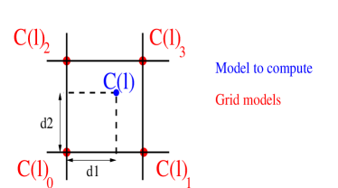
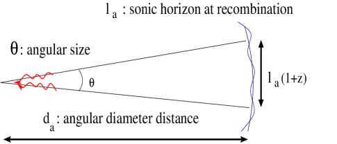
Figure 1: a. left : Linear multidimensional interpolation scheme. b. right : Acoustic scale.

As it is shown on figure 2.a (left), this methods suffers from one major drawback. As we use cosmological models with different cosmological parameters, we sum power spectra with shifted acoustic peaks. The effect is to erase the structure of the peaks, specially at high multipoles.

2.2 Acoustic scale

In order to solve this problem, we use the acoustic scale defined on the figure 1.

With the notation of the figure, the physical size of the acoustic oscillations at decoupling and the angular diameter distance are given by :

$$l_{a}=\int_{t_{eq}}^{t_{rec}}c_{s}dt\ ,\ d_{a}=\frac{1}{\sqrt{\Omega_{K}}}f\left(\sqrt{\Omega_{K}}\int_{0}^{z}\frac{dz}{E(z)}\right),\ \ E(z)=[\Omega_{matter}(1+z)^{3}+\Omega_{curv}(1+z)^{2}+\Omega_{\Lambda}]^{1/2}.$$ (2)

The acoustic scale (in $\ell$-space) is then $as=\pi\frac{d_{a}}{l_{a}}$.

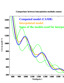
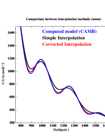
Figure 2: CAMB computed and interpolated power spectra for $\ell=800$ and $\ell=1600$. a. left : Simple multilinear interpolation b. right : Improved interpolation using the acoustic scale.

2.3 Improved interpolation

Our new interpolation scheme is the same as on figure 1.a except that the $\ell$ axis is rescaled according to the ratio of the corresponding acoustic scales. To compute the $C(\ell)$ spectrum for the set of parameter $\{\Omega_{t}\}$ using the $2^{N}$ grid points , we define $2^{N}$ rescaling coefficients $\alpha_{i}(\Omega_{t},\Omega_{i})=as(\Omega_{t})/as(\Omega_{i})$ The interpolated $C(\ell)$ spectrum can then be written as :

$$C_{int}(\ell)=\sum_{i=0}^{2^{N}}w(i)C_{i}(\ell\times\alpha_{i},\ \ \ w(i)=f(d_{1},d_{2}...,d_{n}).$$ (3)

Figure 2.b shows the improvement of the interpolation result, compared to the simple multilinear interpolation.

3 Statistical tests

In order to quantify the improvement of the interpolation, we have computed two statistical quantities :

• we compute the maximum relative difference $Diff_{max}$ between a CAMB computed CMB spectrum and an interpolated one over the $C_{\ell}$ spectrum

• we associate an error $\sigma_{\ell}$ to each point in the $C(\ell)_{int}$, and we compute the $\Delta\chi^{2}$ between this “experiment” and the CAMB original spectrum

  $$Diff_{max}=Max\left(\frac{C(\ell)_{CAMB}-C_{int}(\ell)}{C(\ell)_{CAMB}}\right)_{\ell},\ \ \Delta\chi^{2}=\sum_{\ell=\ell_{min}}^{\ell_{max}}\left(\frac{C(\ell)_{CAMB}-C_{int}(\ell)}{\sigma_{\ell}}\right)^{2}.$$ (4)

Figure 3 presents the distributions obtained for the relative difference and for the $\Delta\chi^{2}$ with error bars similar to the one foreseen for the Planck mission (Puget et al $\!{}^{{\bf?}}$), with $\{\Omega_{t}\}$ randomly distributed over the entire parameter hyperspace. .

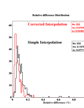
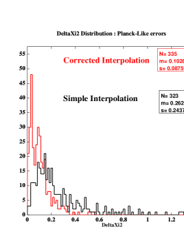
Figure 3: Simple and improved $C(\ell)$ interpolation comparison. a. left : relative difference. b. right :$\Delta\chi^{2}$ for Planck-like error bars.

The reduction in the mean value and the spread of the two quantities ($Diff_{max}$ et $\Delta\chi^{2}$) obtained by the new interpolation show clearly the improvement.

4 Conclusion

We have shown that our improved interpolation method provide a way to diminish the errors introduced in the cosmological parameters estimation process due to the parameter space sampling. Alternatively, for a given precision, it allows to use a smaller grid. It can be useful in the case of future experiments such as the Planck mission. Moreover, the parameter fitting is a fast way of estimating cosmological parameter which can be used in Monte Carlo simulation of an experiment. The impact of the experimental design on the cosmological parameters could then be estimated in this way thanks to the reduction of needed computing resources.

References

References

- [1] Benoit, A. et al. 2003, Astronomy and Astrophysics, 399, L25
- [2] Verde, L. et al. 2003, Astrophysical Journal, 148, 195
- [3] Puget, J.L., High Frequency Instrument for the Planck Mission, response to ESA proposal, 1998.